Different types of integrability and their relation to decoherence in central spin models

Abstract

We investigate the relation between integrability and decoherence in central spin models with more than one central spin. We show that there is a transition between integrability ensured by Bethe ansatz and integrability ensured by complete sets of commuting operators. This has a significant impact on the decoherence properties of the system, suggesting that it is not necessarily integrability or non-integrability which is related to decoherence, but rather its type or a change from integrability to non-integrability.

The Liouville-Arnol’d theorem states that if a system with $n$ degrees of freedom has $n$ involutive integrals of motion, which are functionally independent, its Hamiltonian equations of motion are solvable via quadratures Arnold . Such a system is called integrable. Despite for huge effort, so far it has not been achieved to adapt the concept of integrability to the quantum mechanical framework satisfactorily. At the present time there are two commonly accepted definitions: A quantum mechanical system is called integrable (i) if there is a Bethe ansatz Faddeev or (ii) if the system has a complete set of commuting operators (CSCO) Frahm sharing “suitable” properties (to be further explained below). Note that the notion of integrability in classical mechanics does not require the solvability of the quadratures. In this sense both of the aforementioned approaches are in direct analogy with classical mechanics.

In investigations mainly focused on the first type of integrability, evidence has been found that it is related to transport properties St06 , to quantum phase transitions Emary , and to decoherence Lages05 ; Dahmen . Here systems of the form

$$H=H_{c}+H_{c\leftrightarrow b}+\ldots\text{further terms}$$ (1)

have been considered, where $H_{c}$ denotes a central system and $H_{c\leftrightarrow b}$ a coupling term between the central system and a bath. Mainly two roads have been followed. On the one hand, the influence of chaotic or regular baths on the decoherence of the central system has been investigated Lages05 . On the other hand, the decoherence properties of the central systems of models which are integrable or non-integrable have been studied Dahmen . The usual procedure within such considerations is to evaluate numerically the level statistics of the respective system and to relate a possible change in the statistics to a change of other properties of the system happening at the same point.

Motivated by their important role in the context of solid state quantum information processing SKhaLoss03 , we investigate in the present letter integrability and its relation to decoherence in central spin models. Here we define a quantum system to be integrable if it is possible to compute all eigenstates and eigenvalues of the respective Hamiltonian using operations with less complexity than the direct diagonalization of the Hamiltonian matrix GMann . Here we refer to the computional complexity. The exact diagonalization of a Hamiltonian matrix for example grows exponentially with the system size. This very strict notion of integrability contains (i) and (ii) as possible sources of integrability.

First we study the integrable structure of central spin models. In particular we show that there is a transition between integrability ensured by Bethe ansatz and integrability ensured by CSCO. Differently from the previous investigations described above, we then open a new route by applying a strong magnetic field to the central spin system, and analyze its reaction with respect to decoherence. In the non-integrable case as well as in the case of integrability ensured by Bethe ansatz, the strong magnetic field leads, as generally expected, to highly coherent central spin dynamics, whereas in the remaining case decoherence still takes place. In contrast to previous work we relate the latter observation explicitly to the type of integrability and interpret the result from two different points of view.

The Hamiltonian of a central spin model is given by

$$H = \sum_{i=1}^{N_{c}}\vec{S}_{i}\cdot\sum_{j=1}^{N}A^{i}_{j}\vec{I}_{j}+\sum_{i<j}J_{ij}\vec{S}_{i}\cdot\vec{S}_{j}$$ (2)

$$= \left(\sum_{i=1}^{N_{c}}\vec{S}_{i}\right)\sum_{k=1}^{N}\left(\frac{1}{N_{c}}\sum_{j=1}^{N_{c}}A^{j}_{k}\right)\vec{I}_{k}$$

$$+ \sum_{i=1}^{N_{c}}\sum_{j=i+1}^{N_{c}}\left(\vec{S}_{i}-\vec{S}_{j}\right)\sum_{k=1}^{N}\frac{1}{N_{c}}\left(A^{i}_{k}-A^{j}_{k}\right)\vec{I}_{k}$$

$$+ \sum_{i<j}J_{ij}\vec{S}_{i}\cdot\vec{S}_{j},$$

where in the following we consider $J_{ij}=J$ and $N_{c}>1$. For later convenience we define $A=N_{c}^{-1}\sum_{k=1}^{N}\sum_{j=1}^{N_{c}}A^{j}_{k}$. In the second identity we rewrote the original Hamiltonian into terms of sums and differences between the different central spins. The first term is nothing else than a Gaudin model Gaudin with a central spin replaced by a sum over a set of spins, whereas the second term acts as a perturbation, vanishing whenever $A^{i}_{k}=A^{j}_{k}=:A_{k}$. Hence it has to be expected that this case is integrable, whereas the model generally should be non-integrable. This prediction has been verified explicitly in John09 by a detailed investigation of the spectral statistics of the model. We will come back to the integrable case of two central spins with $A^{1}_{i}=A^{2}_{i}=:A_{i}$ below.

Let us first, however, investigate in more detail general features of the above system, fulfilling $A^{i}_{k}=A^{j}_{k}=:A_{k}$. The central spins can couple to different values of the total central spin squared $\vec{S}^{2}=\left(\sum_{i=1}^{N_{c}}\vec{S}_{i}\right)^{2}$. Fixing the associated quantum number $S$ and defining $\lvert 0\rangle=\lvert S\rangle\lvert I_{1},\ldots,I_{N}\rangle$, we arrive at a usual Gaudin model with eigenstates Garajeu

$$\lvert N_{D}\rangle=\prod_{i=1}^{N_{D}}\left(\omega_{i}S^{-}+\sum_{j=1}^{N}\frac{A_{j}\omega_{i}}{A_{j}-\omega_{i}}I_{j}^{-}\right)\lvert 0\rangle$$ (3)

and eigenvalues

$$E\left(\{\omega_{1},\ldots,\omega_{N_{D}}\}\right)=-2S\sum_{i=1}^{N_{D}}\omega_{i}+S\sum_{j=1}^{N}I_{j}A_{j}.$$ (4)

The parameters $\omega_{i}$ are determined by the Bethe ansatz equations:

$$S+\sum_{j=1}^{N}\frac{A_{j}I_{j}}{A_{j}-\omega_{i}}-2\sum_{k=1,k\neq i}^{N_{D}}\frac{\omega_{k}}{\omega_{k}-\omega_{i}}=0$$ (5)

Here $N_{D}$ is the number of spin flips compared to $\lvert 0\rangle$ Garajeu . Note that these equations are valid for any spin length $S$ and hence any number of central spins $N_{c}$. Considering the Bethe ansatz equations instead of the direct diagonalization of the Hamiltonian matrix reduces a problem of exponential complexity to one of polynomial complexity. Hence the Hamiltonian (2) with $A^{i}_{k}=A^{j}_{k}=:A_{k}$ is integrable, provided the Bethe ansatz equations yield the correct number of solutions $\left\{\omega_{1},\ldots,\omega_{m}\right\}$. This however strongly depends on the inhomogeneity of the couplings $A_{k}$. Indeed for $A_{k}=(A/N)\Leftrightarrow A^{i}_{j}=(A/N)$, the Bethe ansatz equations can never yield all eigenstates and eigenvalues. This becomes clear already on the subspace with only one spin flip. Here the Bethe ansatz equation becomes

$$S+\frac{A}{A-N\omega}\sum_{j=1}^{N}I_{j}=0,$$ (6)

which obviously gives only a single solution.

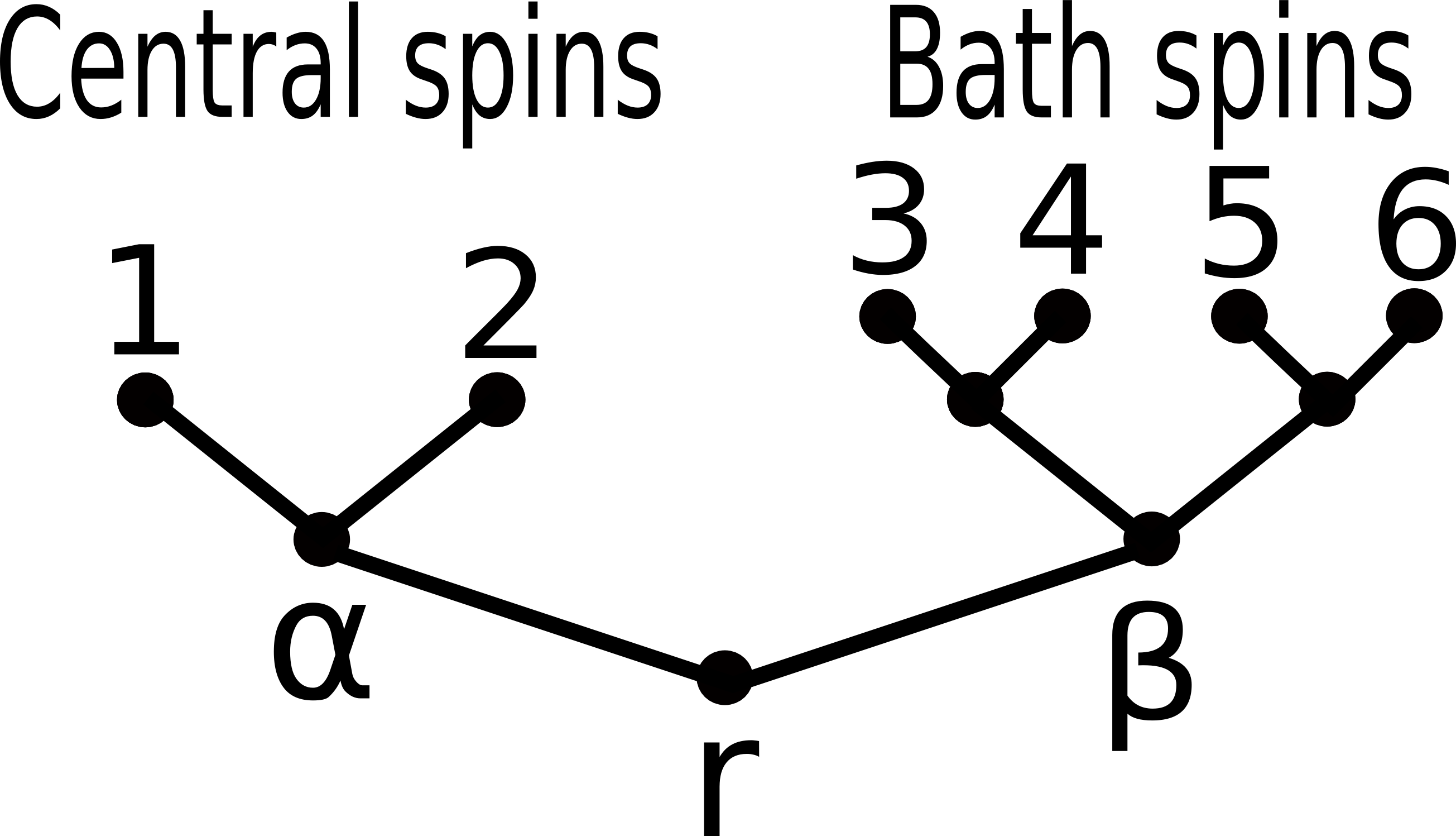
Figure 1: Binary tree with $n=N_{c}+N=2+4=6$ leaves. In order to embed the Hamiltonian of an arbitrary central spin model with homogeneous couplings into a CSCO using the binary tree formalism, two binary trees $\alpha$, $\beta$ with $N_{c}$ and $N$ leaves respectively must be grafted together. The Hamiltonian results as given in (8).

Therefore integrability ensured by Bethe ansatz breaks if all couplings become identical. We now show that in this case integrability is ensured by CSCO. In order to construct the respective operators we apply the so-called binary tree formalism ErbS09 . On the first sight this seems to be unnecessary because Gaudin also gave the following set of operators which together with the Hamiltonian of his central spin model form a CSCO Gaudin :

$$H_{i}=A_{i}\vec{S}\cdot\vec{I}_{i}-\sum_{j=1,j\neq i}^{N}\frac{A_{i}A_{j}\vec{I}_{i}\vec{I}_{j}}{A_{i}-A_{j}}$$ (7)

Indeed these operators, which do not play any role concerning the construction of the eigenstates and eigenvalues of the Gaudin model, obviously become ill-defined in the homogeneous coupling limit. We restrict ourselves to a special case of the binary tree formalism ErbS09 directly adapted to our model: Let $T$ be a binary tree with $n$ leaves as shown in Fig. 1 for $n=6$. A binary tree consists of a set of nodes, each of which is connected to exactly two following nodes, except for the leaves. If we distinguish between a left and a right “child” $p_{1}$ and $p_{2}$ connected to a node $p$, we arrive at a natural ordering of the leaves. We denote the leaves a node $p\in T$ is connected to as $L(p)$. The node connected to all leaves is called the root, denoted by $r$ in the following. Now we associate every leaf $i$ with a spin $\vec{S}_{i}$ and define $H_{p}=\left(\sum_{i\in L(p)}\vec{S}_{i}\right)^{2}$ and $H_{r}^{z}=\sum_{i\in L(r)}S_{i}^{z}$. It is simple to see that for all $p\in T$ these operators commute. As every binary tree with $n$ leaves has $(n-1)$ nodes apart from the leaves, we thus arrive at exactly $n$ non-trivial, mutually commuting operators, which indeed form a CSCO. What makes these operators “suitable” in the sense of the introduction is the fact that they are complete for all spin lengths. In fact for any system it is possible to find a CSCO by e.g. considering the eigenbasis of the respective Hamiltonian and choosing a sufficient number of diagonal matrices with only one entry different from zero. We investigated such systems for the simple model of two Heisenberg coupled spins and found that they consist of more than two operators and lose the property of being complete, when the spin length is changed. We suppose that sets of commuting operators can only be complete for any spin length if the number of operators is equal to the number of spins. Surprisingly, up to our knowledge such a statement has not been made so far.

Now we show how to embed the Hamiltonian of an arbitrary central spin model with homogeneous couplings in a CSCO. To this end we consider two binary trees $\alpha$ and $\beta$ with $N_{c}$ and $N$ leaves respectively. Grafting them together as shown in Fig. 1, we arrive at a new binary tree with $N_{c}+N$ leaves. If we denote $\vec{I}_{i}$ as $\vec{S}_{N_{c}+i}$, the Hamiltonian of the associated homogeneous coupling model can be written in terms of elements of the CSCO resulting from the binary tree formalism as

$$H=\frac{A}{N}(H_{r}-H_{\beta})+\left(\frac{J}{2}-\frac{A}{N}\right)H_{\alpha}.$$ (8)

Note that the number of central and bath spins as well as their lengths are arbitrary and that there is no further restriction to $\alpha$ and $\beta$ so that indeed there are numerous CSCO in which $H$ can be embedded. Furthermore, it should be mentioned that by adding $J_{b}H_{\beta}$ to (8) we can easily include a homogeneous interaction of strength $J_{b}$ between the bath spins. It is simple to find the common eigenstates of the respective CSCO Steini09 ; ErbS09 :

$$\lvert\{S_{p\in T_{L}}\},S^{z}_{r}\rangle$$

$$=\sum_{S^{z}_{p\in T_{r}}}\left(\prod_{p\in T_{L}}\langle S_{p_{1}},S_{p_{2}},S_{p_{1}}^{z},S^{z}_{p_{2}}\lvert S_{p},S_{p}^{z}\rangle\right)$$

$$\lvert S_{1}^{z},\ldots,S_{N+2}^{z}\rangle,$$ (9)

Here $T_{L}=T\setminus L(r)$, $T_{r}=T\setminus r$ and $S_{p}$ denotes the quantum number associated with $H_{p}$. The complexity for calculating the Clebsch-Gordan coefficients is polynomial Loera and hence the approach indeed yields integrability. The eigenvalues read:

$$E(\{S_{p\in T_{L}}\},S^{z}_{r}) = \frac{A}{N}\left(S_{r}(S_{r}+1)-S_{\beta}(S_{\beta}+1)\right)$$ (10)

$$+ \left(\frac{J}{2}-\frac{A}{N}\right)S_{\alpha}(S_{\alpha}+1)$$

Now we relate our above findings to the phenomenon of decoherence. The product of two spin operators consists of flip-flop terms involving ladder operators and a coupling of the $z$-components BJ10 . In the following we evaluate the dynamics for an initial state which is a simple product state. In this case all dynamics and hence all decoherence is purely due to the flip-flop terms. It is well-known that applying a magnetic field $B$ to the central spin system strongly suppresses the influence of flip-flop terms between the central spin system and the bath Coish10 . Here it is usually expected that whenever the magnetic field exceeds all other energy scales $B\gg|A|$, a complete neglect of their influence is justified. In the following we show that the effect of strong suppression of those flip-flop terms actually relies on the inhomogeneity of the couplings and is weakened stronger and stronger the more couplings are chosen to be equal to each other.

To this end in Fig. 2 we consider the special case $N_{c}=2$ with $S_{i}=I_{i}=1/2$ and plot the spin dynamics for two integrable models ($A^{1}_{j}=A^{2}_{j}=:A_{j}$, as explained above) with inhomogeneous and homogeneous coupling costants. In the first case the coupling constants $A_{j}$ are chosen with respect to a non-uniform distribution so that $A_{i}\neq A_{j}$. For our initial state this case can only be accessed via exact diagonalization, strongly restricting the size of the system SKhaLoss03 . We therefore illustrate the two situations considering a comparatively small system with $N=2N_{D}+1$ and $N_{D}=5$. This corresponds to a very low bath polarization of $1/N$. The initial state of the central spin system is $\lvert\Uparrow\Downarrow\rangle$. We checked the dynamics for much larger systems in the homogeneous case using a semi-analytical approach based on BJ10 and did not find any qualitative differences. Moreover, non-integrable systems with fully inhomogeneous couplings $A^{i}_{k}\neq A^{j}_{k}$ show a qualitatively very similar behavior to the integrable case of inhomogeneous couplings, $A^{1}_{i}=A^{2}_{i}=:A_{i}$ and $A_{i}\neq A_{j}$. Note that all results derived for the special case of $N_{c}=2$ and $S_{i}=I_{i}=1/2$ in the following can be directly adapted to the general case of an arbitrary number of central spins and arbitrary spin lengths.

Although the magnetic field is in both cases larger than any other energy scale, the dynamics for the inhomogeneous case is completely coherent, whereas in the other case it still decays. This means that in the inhomogeneous case the flip-flop terms between the central spin system and the bath do not contribute to the dynamics in any determinable way. The oscillations are completely due to the flip-flop terms between the two central spins.

Figure 2: Spin dynamics for $N_{c}=2$, $N=2N_{D}+1=11$, where $S_{i}=I_{i}=(1/2)$, and $B=3.441A$, $J=0.023A$. The initial state of the system is $\lvert\Uparrow\Downarrow\rangle\otimes\prod_{i=1}^{N_{D}}I^{-}_{i}\lvert 0\rangle$. We consider two integrable models fulfilling $A^{1}_{i}=A^{2}_{i}=:A_{i}$ with either $A_{i}\neq A_{j}$ (upper panel), chosen due to a non-uniform distribution, or $A_{i}=A_{j}$ (lower panel). Although in both cases $B$ is larger than any other energy scale, for homogeneous couplings the dynamics still decays, indicating decoherence.

A qualitative explanation of the above effect goes as follows: Flipping a spin in a magnetic field changes the energy $E$ by $\Delta E\propto B$. In order to ensure energy conservation this change must be compensated. As indicated in the upper sketch of Fig. 3, for inhomogeneous couplings this has to be done by the energy change due to the flip of the respective bath spin and the one resulting from the central spin flip via the central spin coupling term. Hence if the magnetic field exceeds any other energy scale, this is impossible and flip-flop processes are forbidden by energy conservation (at least in first-order time-dependent perturbation theory).

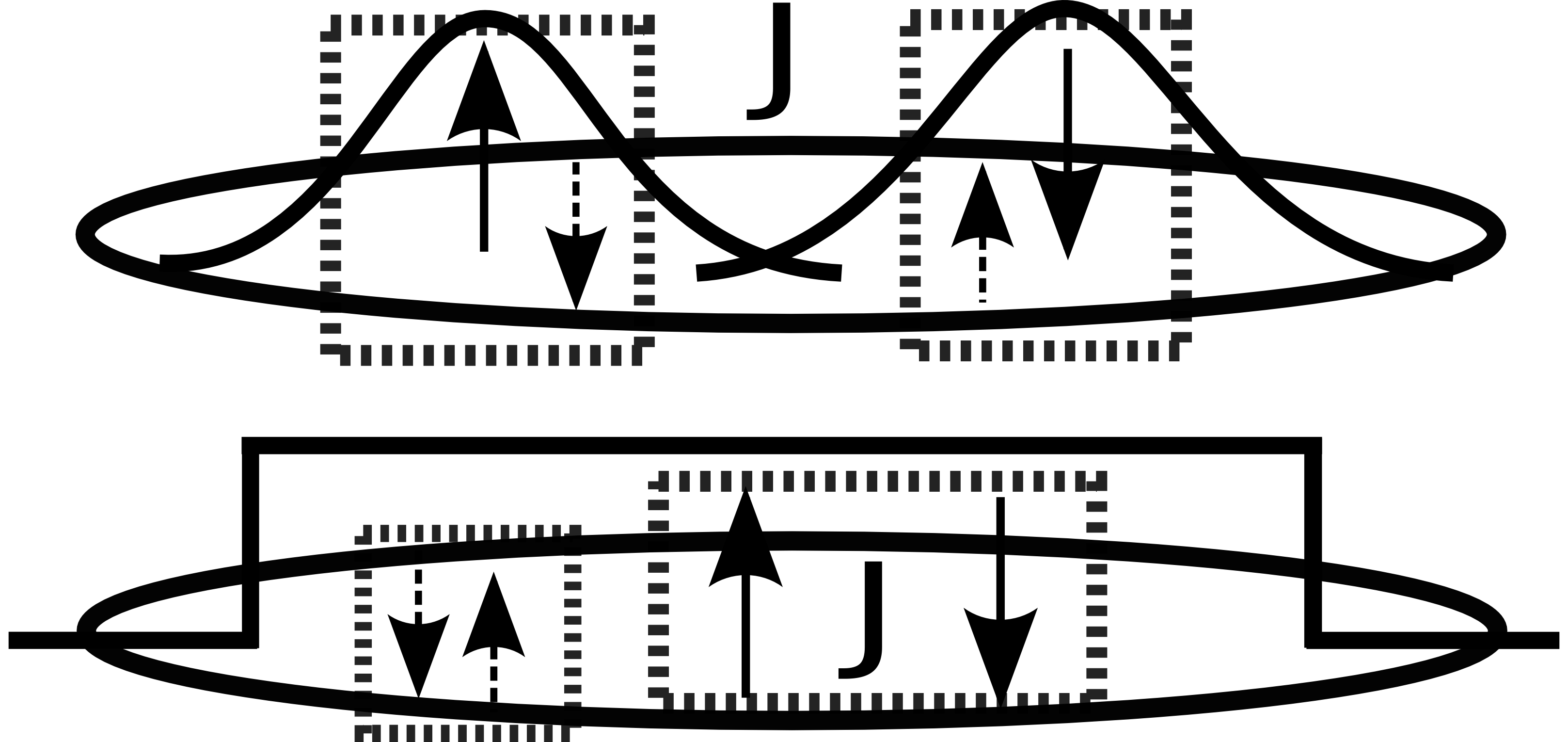
Figure 3: Sketch of flip-flop processes in a $N_{c}=2$ central spin system with inhomogeneous (upper panel) and homogeneous (lower panel) couplings. For homogeneous couplings, the energy changes due to simultaneous central and nuclear spin flips can compensate each each other. This is not possible for inhomogeneous couplings because the energies of flips differ for different nuclear spins.

If we instead consider homogeneous couplings, this restriction can be circumvented by simultaneous flip-flop processes on both of the central spins. Here the energy changes due to the central spin flips in the magnetic field and the bath spin flips compensate each other as depicted in the second sketch of Fig. 3. This is impossible for inhomogeneous couplings because the energy change depends on which bath spin is flipped.

This simple effect vanishes for initial states with a fully polarized central or nuclear spin system. However, from the above explanation it is clear it will still occur if the couplings are varied away slightly from complete homogeneity. This means that the more the couplings approach the CSCO integrable limit, the less flip-flop terms are suppressed by a magnetic field applied to the central spin system. This leads to two different interpretations of the results, both of which indicate that it is not necessarily the integrability or non-integrability itself which is related to decoherence, as assumed in previous studies Lages05 ; Dahmen : (a) As demonstrated above, the influence of a magnetic field applied to the central spin system on the decoherence properties strongly differs for models which are clearly non-integrable or integrable by Bethe ansatz and those which are near to the CSCO integrable limit. In the first case the dynamics becomes highly coherent, whereas in the second case it still decays. This suggests that it is the mathematical structure ensuring integrability, which determines the reaction of a system on an external quantity applied to the central system with respect to the decoherence properties rather than the integrability or non- integrability itself. (b) An even more general interpretation results from the observation that if we apply a magnetic field to the central spin system, the non-integrable models as well as those integrable by Bethe ansatz keep the respective property, whereas it is lost in the CSCO case. Hence the result suggests that if a model is close to a limit in which the integrability is broken by some external quantity applied to the central system, its decoherence properties will be stronger affected than those of a system near to a limit with stable integrability. It is therefore the breaking of integrability which has a negative effect on the decoherence properties and not the actual integrability or non-integrability.

Of course our results have to be regarded as a first indication into this direction and it would be desirable to check them for more general external quantities on a wider class of systems. As explained above, in (8) we can easily add a term describing an interaction between the different bath spins. Hence in an immediate next step it would be interesting to check for which types of bath terms the Bethe ansatz integrability still holds and if we can find effects similar to those described in this paper. In this context see e.g. Ref. Lages05 .

- (1) V. I. Arnol‘d, Mathematical Methods of Classical Mechanics, (Springer, Berlin 1978).
- (2) see e.g. L. D. Faddeev, arXiv:9605187 (1995).
- (3) see e.g. H. Frahm, J. Phys. A: Math. Theor. 26, L473 (1993).
- (4) R. Steinigeweg, J. Gemmer, and M. Michel, Europhys. Lett. 75(3), 406 (2006).
- (5) C. Emary and T. Brandes, Phys. Rev. Lett. 90, 044101 (2003)
- (6) J. Lages et al., Phys. Rev. E 72, 026225 (2005); A. Relano, J. Dukelsky, and R. A. Molina, Phys. Rev. E 76, 046223 (2007).
- (7) S. R. Dahmen et al., J. Stat. Mech., P10019 (2004); K. Kudo and T. Deguchi, Phys. Rev. B, 68, 052510 (2003); R. M. Angelo et al., Phys. Rev. E 60, 5 (1999); T. Gorin and T. H. Seligman, Phys. Lett. A 309, 61-67 (2003).
- (8) J. Schliemann, A. Khaetskii, and D. Loss , J. Phys.: Condens. Mat. 15, R1809 (2003); W. Zhang et al., J. Phys.: Condens. Mat. 19, 083202 (2007); W. A. Coish and J. Baugh, phys. stat. sol. B 246, 2203 (2009); J. M. Taylor et al., Phys. Rev. B 76, 035315 (2007).
- (9) F. H. L. Essler et al., The one-dimensional Hubbard model, (Cambridge University Press, 2005).
- (10) M. Gaudin, J. Phys. (Paris) 73, 1087 (1976).
- (11) J. Schliemann, Phys. Rev. B 81, 081301(R) (2010).
- (12) D. Garajeu and A. Kiss, J. Math. Phys. 42, 3497 (2001).
- (13) B. Erbe and H.-J. Schmidt, J. Phys. A: Math. Theor. 43, 085215 (2010).
- (14) R. Steinigeweg and H.-J. Schmidt, Mathematical Physics, Analysis and Geometry 12(1), 19 (2009).
- (15) J. A. De Loera and T. B. McAllister, Exp. Math. 15, 1 (2006).
- (16) B. Erbe and J. Schliemann, Phys. Rev. B 81, 235324 (2010).
- (17) see e.g. W. A. Coish, J. Fischer, and D. Loss, Phys. Rev. B 81, 165315 (2010).