Charm-loop effect in $B\to K^{(*)}\ell^{+}\ell^{-}$ and $B\to K^{*}\gamma$

Abstract:

We calculate the long-distance effect generated by the four-quark operators with $c$-quarks in the $B\to K^{(*)}\ell^{+}\ell^{-}$ decays. At the lepton-pair invariant masses far below the $\bar{c}c$-threshold, $q^{2}\ll 4m_{c}^{2}$, we use OPE near the light-cone. The nonfactorizable soft-gluon emission from $c$-quarks is cast in the form of a nonlocal effective operator. The $B\to K^{(*)}$ matrix elements of this operator are calculated from the QCD light-cone sum rules with the $B$-meson distribution amplitudes. As a byproduct, we also predict the charm-loop contribution to $B\to K^{*}\gamma$ beyond the local-operator approximation. To describe the charm-loop effect at large $q^{2}$, we employ the hadronic dispersion relation with $\psi=J/\psi,\psi(2S),...$ contributions, where the measured $B\to K^{(*)}\psi$ amplitudes are used as inputs. Matching this relation to the result of QCD calculation reveals a destructive interference between the $J/\psi$ and $\psi(2S)$ contributions. The resulting charm-loop effect is represented as a $q^{2}$-dependent correction $\Delta C_{9}(q^{2})$ to the Wilson coefficient $C_{9}$. Within uncertainties of our calculation, at $q^{2}$ below the charmonium region the predicted ratio $\Delta C_{9}(q^{2})/C_{9}$ is $\leq 5\%$ for $B\to K\ell^{+}\ell^{-}$, but can reach as much as 20% for $B\to K^{*}\ell^{+}\ell^{-}$, the difference being mainly caused by the soft-gluon contribution.

1 Introduction

Being very prospective channels for the search for new physics, the exclusive $B\to K^{(*)}\ell^{+}\ell^{-}$ decays have quite a complicated dynamics. In the Standard Model the underlying flavour-changing $b\to s\ell^{+}\ell^{-}$ transition is described by the effective Hamiltonian [1, 2]:

$$H_{eff}=-\frac{4G_{F}}{\sqrt{2}}V_{tb}V_{ts}^{*}{\sum\limits_{i=1}^{10}}C_{i}({\mu})O_{i}({\mu})\,,$$ (1)

a superposition of the effective operators $O_{i}$, weighted by their Wilson coefficients $C_{i}$ and normalized at the scale $\mu\sim m_{b}$. The relevant operators are presented in Appendix A. In this paper we neglect the CKM-suppressed contributions proportional to $V_{ub}V_{us}^{*}$, adopting the approximation $|V_{tb}V_{ts}^{*}|\simeq|V_{cb}V^{*}_{cs}|=0.0428^{+0.001}_{-0.004}$ [3].

The decay amplitude

$$A(B\to K^{(*)}\ell^{+}\ell^{-})=-\langle K^{(*)}\ell^{+}\ell^{-}\mid H_{eff}\mid B\rangle\,,$$ (2)

contains a rich variety of hadronic matrix elements of the operators $O_{i}$. The dominant contributions to (2) are generated by the $O_{9,10}$ and $O_{7\gamma}$ with large Wilson coefficients. In Appendix B the hadronic matrix elements of these operators are presented. They are factorized in terms of the $B\to K^{(*)}$ form factors, which, similar to the $B\to\pi,\rho$ form factors of the weak semileptonic decays, are obtained from lattice QCD or QCD light-cone sum rules (LCSR). In addition, there are specific contributions to the $B\to K^{(*)}\ell^{+}\ell^{-}$ and $B\to K^{*}\gamma$ amplitudes generated by the current-current operators, $O_{1,2}$ and penguin operators $O_{3-6,8g}$, combined with the electromagnetic (e.m.) interaction of quarks. A major challenge for the theory is to identify and estimate these hadronic matrix elements one by one.

An important effect, which is the main topic of our study, is generated by the current-current operators $O_{1,2}$ acting together with the $c$-quark e.m. current. This mechanism involves an intermediate “charm-loop”, coupled to the lepton pair via the virtual photon. The analogous effects for the $u$-quark current-current and quark-penguin operators with different flavours are not important in $B\to K^{(*)}\ell^{+}\ell^{-}$, being either CKM suppressed, or multiplied by a small Wilson coefficient.

The $c$-quark loop turns into a genuine long-distance hadronic effect if the lepton-pair invariant mass $q^{2}=(p_{\ell^{+}}+p_{\ell^{-}})^{2}$ reaches the region of charmonium resonances $\psi=\{J/\psi,\psi(2S),....\}$. At $q^{2}=m_{\psi}^{2}$, the process $B\to K^{(*)}\ell^{+}\ell^{-}$ transforms into a nonleptonic weak decay $B\to\psi K^{(*)}$, followed by the leptonic annihilation of $\psi$. All $\psi$-resonances with $m_{\psi}<(m_{B}-m_{K^{(*)}})$ contribute to this mechanism. Moreover, above the $\bar{D}D$ threshold there are continuum contributions of the intermediate charmed hadrons and it is very difficult to include them in a model-independent way. Although the $q^{2}$-intervals around $J/\psi$ and $\psi(2S)$ are subtracted from the measured lepton-pair mass distributions in $B\to K^{(*)}\ell^{+}\ell^{-}$, the intermediate and/or virtual $\bar{c}c$ states contribute outside the resonance region and their effect has to be accurately estimated.

Usually, in the leading-order, the $c$-quark loop diagram is included into the factorization formula for $B\to K^{(*)}\ell^{+}\ell^{-}$. In addition, hard-gluon exchanges between the $c$-quark loop and the rest of the diagram are taken into account, together with other perturbative nonfactorizable effects (see e.g., [4]). One generally predicts these effects to be small, if $q^{2}$ is far below the charmonium region.

Two important questions concerning the charm-loop effect remain unanswered, despite many dedicated studies. The first question is: how important are the soft gluons emitted from the $c$-quark loop and violating the factorization? The second question concerns the validity of the approximation “$c$-quark-loop plus corrections” at large $q^{2}$, approaching the charmonium resonance region. It is the purpose of our paper to address these questions.

The soft-gluon emission from the charm loop was calculated for the inclusive $B\to X_{s}\gamma$ decay in [5] and, independently, for the exclusive channel $B\to K^{*}\gamma$ in [6]. The main outcome was an effective quark-antiquark-gluon operator whose Wilson coefficient is proportional to $1/m_{c}^{2}$. In $B\to K^{*}\gamma$ the hadronic matrix element of this operator was obtained [6] using three-point QCD sum rules and, more recently, LCSR [7]. Studies of this effect in $B\to X_{s}\gamma$ and $B\to X_{s}\ell^{+}\ell^{-}$ [8] revealed that, in addition to the lowest-dimension local operator, a tower of operators with the derivatives of the gluon field has to be taken into account. Explicitly, the soft-gluon momentum was taken into account in [9] for the inclusive decay $B\to X_{s}\ell^{+}\ell^{-}$.

In this paper we employ operator-product expansion (OPE) near the light-cone for the gluon emission from the $c$-quark loop at $q^{2}\ll 4m_{c}^{2}$. From this expansion we derive an effective nonlocal quark-antiquark-gluon operator. Sandwiching this operator between the $B$ and $K^{(*)}$ states we calculate the hadronic matrix elements employing LCSR with $B$-meson distribution amplitudes. These sum rules have been used in [10, 11] to obtain the $B\to$ light-meson form factors. The calculation presented below provides an effective resummation of the soft-gluon part of the charm-loop effect in $B\to K^{(*)}\ell^{+}\ell^{-}$ and (as a byproduct) in $B\to K^{*}\gamma$. Adding the calculated soft-gluon contribution to the leading-order factorizable $\bar{c}c$ loop , we obtain an estimate of the charm-loop effect in $B\to K^{(*)}\ell^{+}\ell^{-}$, valid at $q^{2}\ll 4m_{c}^{2}$.

The second problem investigated in this paper is the validity of OPE at large $q^{2}$, approaching the charmonium region. This issue is closely related to the status of quark-hadron duality for the charm-loop amplitude. Earlier models [12], adding the contributions of $\psi$-resonances on the top of the $c$-quark loop, involve double counting of quark-gluon and hadronic degrees of freedom. More consistent is the use of the hadronic dispersion relation written in terms of $\psi$ states, as suggested for $B\to X_{s}\ell^{+}\ell^{-}$ in [13]. Recently, this approach was reconsidered in [14]. In all previous analyses involving dispersion relation, nonfactorizable contributions to the charm-loop effect were neglected, and, correspondingly, the nonleptonic $B\to\psi K^{(*)}$ amplitudes were taken in the factorization approximation. In order to adjust these amplitudes to their measured values, additional $k$-factors were introduced [13, 15].

In this paper we employ the hadronic dispersion relation in a different way. We fix the absolute values of residues of the $J/\psi$- and $\psi(2S)$-poles from the experimental data on $B\to J/\psi K^{(*)},\psi(2S)K^{(*)}$. The integral over the spectral density above the open charm threshold is parameterized in a form of an effective pole. We then fit the whole dispersion relation to the OPE result at $q^{2}\ll 4m_{c}^{2}$, including the newly calculated nonfactorizable contribution. Importantly, we find that this procedure favours a destructive interference between the $\psi(2S)$ and $J/\psi$ terms in the dispersion relation. Our main result for the charm-loop effect is obtained in terms of the $q^{2}$- and process-dependent correction to the Wilson coefficient $C_{9}$. This correction is directly calculated at small $q^{2}$ and analytically continued to large $q^{2}<m_{\psi(2S)}^{2}$ via OPE-controlled dispersion relation.

The plan of this paper is as follows. Sect. 2 contains an introductory discussion of the OPE for the charm-loop effect. In Sect. 3 we expand the product of the four-quark operators with the $c$-quark e.m. current near the light cone and obtain the non-local operator corresponding to the nonfactorizable soft-gluon emission. Sect. 4 contains the derivation of LCSR for the $B\to K$ and $B\to K^{*}$ matrix elements of this operator. Adding them to the known factorizable matrix elements, we obtain the full charm-loop contribution to $B\to K^{(*)}\ell^{+}\ell^{-}$, valid at small $q^{2}$. In Sect. 5 we present the details of our numerical analysis and obtain the results for the charm-loop effect in a form of the correction to $C_{9}$. Sect. 6 contains our prediction for the charm-loop effect in $B\to K^{*}\gamma$. In Sect. 7 we perform the matching of the OPE result to the hadronic dispersion relation in terms of charmonium resonances, predicting the charm-loop effect at $q^{2}$ up to the open charm threshold. Finally, we investigate the influence of this effect on the observables of $B\to K^{(*)}\ell^{+}\ell^{-}$. Sect. 8 contains the concluding discussion. In Appendix A the effective operators and their Wilson coefficients are collected. In Appendix B the definitions of $B\to K^{(*)}\ell^{+}\ell^{-}$ amplitudes and the inputs for form factors are presented. In Appendix C the relevant characteristics of $J/\psi$ , $\psi(2S)$ states and $B\to K^{(*)}J/\psi(\psi(2S))$ decays are given. In Appendix D the expressions for the coefficients entering the LCSR are presented.

2 Light-cone dominance of the c-quark loop

The combined action of the four-quark operators $O_{1}$ and $O_{2}$ in (1) and the e.m. interactions of $c$-quarks and leptons leads to the charm-loop effect depicted in Fig. 1.

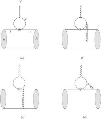
Figure 1: Charm-loop effect in $B\to K^{(*)}\ell^{+}\ell^{-}$: (a)-the leading-order factorizable contribution; (b) nonfactorizale soft-gluon emission, (c),(d)-hard gluon exchange.

The contribution of this mechanism to the $B\to K^{(*)}\ell^{+}\ell^{-}$ decay amplitude can be written as

$$A(B\to K^{(*)}\ell^{+}\ell^{-})^{(O_{1,2})}=-(4\pi\alpha_{em}Q_{c})\frac{4G_{F}}{\sqrt{2}}V_{tb}V^{*}_{ts}\frac{\bar{\ell}\gamma^{\mu}\ell}{q^{2}}{\cal H}_{\mu}^{(B\to K^{(*)})}(p,q)\,,$$ (3)

where $Q_{c}=2/3$ is the $c$-quark electric charge, the lepton current and photon propagator are factored out and the hadronic transition matrix element is:

$${\cal H}^{(B\to K^{(*)})}_{\mu}(p,q)=i\int d^{4}xe^{iq\cdot x}\langle K^{(*)}(p)|T\Big{\{}\bar{c}(x)\gamma_{\mu}c(x)\,,$$

$$\Big{[}C_{1}O_{1}(0)+C_{2}O_{2}(0)\Big{]}\Big{\}}|B(p+q)\rangle\,.$$ (4)

Isolating in (4) the $T$-product of the $c$-quark e.m. current and the $c$-quark fields entering $O_{1}$ or $O_{2}$, one has in both cases a generic expression:

$${\cal C}^{a}_{\mu}(q)=\int d^{4}xe^{iq\cdot x}T\Big{\{}\bar{c}(x)\gamma_{\mu}c(x),\bar{c}_{L}(0)\Gamma^{a}c_{L}(0)\Big{\}}\,,$$ (5)

where $\Gamma^{a}$ denotes a certain combination of Dirac- and colour-matrices.

At $q^{2}\ll 4m_{c}^{2}$, that is, if $c$-quarks are highly virtual, the dominant region of integration over $x$ in (5) is concentrated near the light-cone $x^{2}=0$. To see that, we follow [11], where the light-cone dominance of the correlation functions containing one heavy-quark field was demonstrated. Taking $q^{2}$ small but time-like, it is convenient to consider the rest frame of the virtual photon with $q=(q_{0},\vec{0})$, defining a unit vector $w=q/\sqrt{q^{2}}=(1,\vec{0})$, $w^{2}=1$. The virtual $c$-quark fields in (5) are then decomposed into the static part and residual 4-momentum: $p_{c}=m_{c}w+\tilde{p}$, so that $c(x)=\exp(-im_{c}w\cdot x)h_{w}(x)$, where the effective field $h_{w}(x)$ contains only the $\tilde{p}$ components. Note that the last redefinition only aims at separating the $m_{c}$ scale from the virtual $c$-quark momentum and making the residual off-shell momentum $\tilde{p}$ independent of this scale. Since the virtual $\bar{c}$ quark 4-momentum is $p_{\bar{c}}=q-p_{c}=q-(m_{c}w+\tilde{p})$, the $m_{c}w$ component of the Dirac-conjugated $\bar{c}$-field enters with the same sign, so that $\bar{c}(x)=\exp(-im_{c}w\cdot x)\bar{h}_{w}(x)$. After rescaling all $c$ and $\bar{c}$ fields, the operator (5) transforms to

$${\cal C}^{a}_{\mu}(q)=\int d^{4}xe^{-i(2m_{c}w-q)\cdot x}T\Big{\{}\bar{h}_{w}(x)\gamma_{\mu}h_{w}(x),\bar{h}_{wL}(0)\Gamma^{a}h_{wL}(0)\Big{\}}\,,$$ (6)

where the $m_{c}$-dependence is now concentrated in the exponent. In the above integral, the dominant contribution stems from the region where the exponent does not strongly oscillate, that is, where $(2m_{c}w-q)\cdot x\sim 1$ , yielding

$$\langle x^{2}\rangle\sim 1/(2m_{c}w-q)^{2}\sim 1/(2m_{c}-\sqrt{q^{2}})^{2}\,,$$ (7)

(for a more detailed derivation see e.g., [16]). In the region $q^{2}\ll 4m_{c}^{2}$ the light-cone OPE for the product of operators in (6) can be applied. When $q^{2}$ grows and approaches the threshold $4m^{2}_{c}$, the expansion becomes invalid. Note that due to Lorentz-invariance, the estimate (7) is valid in any frame, including the rest frame of $B$-meson, where both the $c$-quark pair and $s$ quark emitted in the heavy $b$-quark decay, are energetic.

3 Expansion near the light-cone

The expansion of the operator-product in (5) starts with contracting the $c$-quark fields in the free propagators forming a two-point $c$-quark loop. At leading order, there is no difference between the light-cone and local OPE and the hadronic matrix element is:

$$\Big{[}{\cal H}^{(B\to K^{(*)})}_{\mu}(p,q)\Big{]}_{fact}=\left(\frac{C_{1}}{3}+C_{2}\right)\langle K^{(*)}(p)|{\cal O}_{\mu}(q)|B(p+q)\rangle\,,$$ (8)

where both $O_{1}$ and $O_{2}$ contribute and the local operator

$${\cal O}_{\mu}(q)=(q_{\mu}q_{\rho}-q^{2}g_{\mu\rho})\frac{9}{32\pi^{2}}~{}g(m_{c}^{2},q^{2})\bar{s}_{L}\gamma^{\rho}b_{L}\,.$$ (9)

is reduced to the $b\to s$ current. Hence the matrix element (8) is factorized to $B\to K^{(*)}$ form factors. Diagrammatically, this contribution is shown in Fig. 1a. The charm-loop coefficient function in (9) in the adopted operator basis is given by the well-known expression [1]:

$$g(m_{c}^{2},q^{2}) = -\frac{8}{9}\ln\left(\frac{m_{c}}{m_{b}}\right)+\frac{8}{27}+\frac{4}{9}y(q^{2})$$ (10)

$$-\frac{4}{9}\left(2+y(q^{2})\right)\sqrt{y(q^{2})-1}~{}\mbox{arctan}\left(\frac{1}{\sqrt{y(q^{2})-1}}\right)\,,$$

where $y(q^{2})=4m_{c}^{2}/q^{2}>1$, the renormalization scale is taken as $m_{b}$ and $g(m_{c}^{2},0)=-8/9\ln(m_{c}/m_{b})-4/9$. Furthermore, a dispersion relation for the coefficient function in the variable $q^{2}$ is valid:

$$g(m_{c}^{2},q^{2})=g(m_{c}^{2},0)+\frac{q^{2}}{\pi}\int\frac{\mbox{Im}_{s}g(m_{c}^{2},s)}{s(s-q^{2})}ds\,.$$ (11)

with the spectral density:

$$\frac{1}{\pi}\,\mbox{Im}_{s}g(m_{c}^{2},s)=\frac{4}{9}\sqrt{1-\frac{4m_{c}^{2}}{s}}(1+\frac{2m_{c}^{2}}{s})\Theta(s-4m_{c}^{2})~{}.$$ (12)

The factorizable amplitude (8) is often called “perturbative” or “short-distance” charm-loop effect. There are gluon corrections to this amplitude which do not violate factorization. For instance, the perturbative gluon exchanges within the $c$-quark loop in Fig. 1a are known and can in principle be added in a form of $O(\alpha_{s})$ corrections to the coefficient function $g(m_{c}^{2},q^{2})$. We will neglect them here. The $O(\alpha_{s})$ corrections to the weak-current vertex are implicitly included in the calculation of the hadronic form factors, e.g., in LCSR [17, 18].

The nonfactorizable contributions to the hadronic matrix element (4) start with the one-gluon emission from the charm-loop. Some of the nonfactorizable diagrams with hard-gluon exchanges in $O(\alpha_{s})$ are shown in Fig. 1c,d. They are included in the NLO factorization formula [4], (see also [19]) for $B\to K^{(*)}\ell^{+}\ell^{-}$ or $B\to K^{*}\gamma$ in a form of the hard-scattering kernels convoluted with the $B$- and $K^{*}$-meson light-cone distribution amplitudes (DA’s). These perturbative effects can be taken into account separately and will not be included in our analysis. Nonfactorizable two-gluon effects in (9) with one hard and one soft gluon, or with two hard gluons are also neglected, being presumably very small due to extra $O(\alpha_{s})$ suppression.

In this paper, we consider the emission of one soft gluon (with low virtuality but nonvanishing momentum) from the $c$-quark loop and evaluate the contribution of this mechanism to the $B\to K^{(*)}\ell^{+}\ell^{-}$ amplitudes. One of the corresponding diagrams is shown in Fig. 1b, the second one has a gluon emitted from the other $c$-quark line.

In terms of the light-cone expansion, the contraction of $c$-quark fields entering (4) yields a gluon-field operator multiplied by a $b\to s$ colour-octet current. Note that only the operator $O_{1}$ contributes at this level. In order to calculate this contribution we use the $c$-quark propagator near the light-cone [20] including the one-gluon term:

$$\langle 0\mid T\{c(x_{1})\bar{c}(x_{2})\}\mid 0\rangle=-i\int\frac{d^{4}k}{(2\pi)^{4}}e^{-ik(x_{1}-x_{2})}\frac{/\!\!\!k+m_{c}}{m_{c}^{2}-k^{2}}$$

$$-i\!\int\limits_{0}^{1}duG^{\alpha\beta}(ux_{1}+\bar{u}x_{2})\!\!\int\!\!\frac{d^{4}k}{(2\pi)^{4}}e^{-ik(x_{1}-x_{2})}\frac{\bar{u}(/\!\!\!k+m_{c})\sigma_{\alpha\beta}+u\sigma_{\alpha\beta}(/\!\!\!k+m_{c})}{2(m_{c}^{2}-k^{2})^{2}}\,,$$ (13)

where $G^{\alpha\beta}(x)=g_{s}(\lambda^{a}/2)G^{a\,\alpha\beta}(x)$, $\bar{u}=1-u$, and the fixed-point gauge for the gluon field is used. The above symmetric form can easily be derived from the expression presented, e.g., in [21].

To proceed, we define the light-cone kinematics in the rest-frame of the decaying $B$-meson, introducing the unit vector $v=p_{B}/m_{B}=(p_{K^{(*)}}+q)/m_{B}=(1,0,0,0)$, two light-cone vectors $n_{\pm}$, so that :

$$v = \frac{1}{2}(n_{+}+n_{-})\,,\qquad n_{+}^{2}=n_{-}^{2}=0\,,\qquad(n_{+}n_{-})=2\,,$$

$$q = (n_{-}q){n_{+}\over 2}+(n_{+}q){n_{-}\over 2}\,,$$ (14)

and choosing $\vec{q}_{\perp}=0$. We consider a kinematical situation when the lepton-pair invariant mass is small: $q^{2}=(n_{+}q)(n_{-}q)\ll 4m_{c}^{2}<m_{b}^{2}$ , while $(vq)=1/2[(n_{+}q)+(n_{-}q)]\sim m_{b}/2$ is large, so that one of the components of $q$ in the above expansion dominates, or equivalently, $q$ is approximately parallel to one of the light-cone directions. We choose

$$(n_{-}q)\sim m_{b},\quad(n_{+}q)\sim\frac{q^{2}}{m_{b}}\ll(n_{-}q),\quad\mbox{hence}\quad q\simeq(n_{-}q)\frac{n_{+}}{2}\,.$$ (15)

The propagator (13) taken between $x$ and $0$ involves the gluon field at the point $ux$, $(0<u<1)$ which we rewrite via nonlocal differential operator:

$$G^{\alpha\beta}(ux)=\exp[-iux_{\tau}(i{\cal D}^{\tau})]\,\,G^{\alpha\beta}\,.$$ (16)

where $G^{\alpha\beta}=G^{\alpha\beta}(0)$. Note that due to the fixed-point gauge, the simple derivative can be replaced by the covariant derivative acting on the gluon field and ensuring gauge invariance.

We are interested in the dominant effect of the nonvanishing gluon momenta generated by the exponent in (16). Decomposing the covariant derivative in the light-cone vectors

$${\cal D}=(n_{+}{\cal D})\frac{n_{-}}{2}+(n_{-}{\cal D})\frac{n_{+}}{2}+{\cal D}_{\perp},$$ (17)

we retain only the $n_{-}$ component, which corresponds to the gluons emitted antiparallel to $q$, that is, in the same direction as the $s$-quark in the $B$-meson rest frame. We then have

$$G^{\alpha\beta}(ux) \simeq \exp[-iu(n_{-}x){(in_{+}{\cal D})\over 2}]G^{\alpha\beta}$$ (18)

$$= \int d\omega\,\exp[-iu(n_{-}x)\omega]\,\delta[\omega-{(in_{+}{\cal D})\over 2}]\,\,G^{\alpha\beta}\,.$$

Inserting this expression in the propagator (13), and shifting the $k$ integration, we obtain for the one-gluon part of the propagator:

$$\langle 0\mid T\{c(x)\bar{c}(0)\}\mid 0\rangle_{G}=-i\int d\omega\int\limits_{0}^{1}du\int\frac{d^{4}k}{(2\pi)^{4}}\exp\left(-ikx\right)$$

$$\times\frac{\bar{u}(/\!\!\!k+m_{c}-u/\!\!\!n_{-}\omega)\sigma_{\alpha\beta}+u\sigma_{\alpha\beta}(/\!\!\!k+m_{c}-u/\!\!\!n_{-}\omega)}{2(m_{c}^{2}-[k-un_{-}\omega]^{2})^{2}}\delta[\omega-{(in_{+}{\cal D})\over 2}]G^{\alpha\beta}\,.$$ (19)

Using this form of the propagator in (4), we cast the soft-gluon emission part of the hadronic matrix element in a form:

$$\Big{[}{\cal H}^{(B\to K^{(*)})}_{\mu}(p,q)\Big{]}_{nonfact}=2C_{1}\langle K^{(*)}(p)|\widetilde{{\cal O}}_{\mu}(q)|B(p+q)\rangle\,,$$ (20)

where $\widetilde{{\cal O}}_{\mu}(q)$ is a convolution of the coefficient function with the nonlocal operator:

$$\widetilde{{\cal O}}_{\mu}(q)=\int d\omega\,I_{\mu\rho\alpha\beta}(q,\omega)\bar{s}_{L}\gamma^{\rho}\delta[\omega-{(in_{+}{\cal D})\over 2}]\widetilde{G}_{\alpha\beta}b_{L}\,\,.$$ (21)

In the above, $\widetilde{G}_{\alpha\beta}=\frac{1}{2}\epsilon_{\alpha\beta\sigma\tau}G^{\sigma\tau}$, and the derivative acts only on the gluon-field operator. The coefficient function reads:

$$I_{\mu\rho\alpha\beta}(q,\omega) = {1\over 8\pi^{2}}\int_{0}^{1}du\Big{\{}\Big{[}\bar{u}\tilde{q}_{\mu}\tilde{q}_{\alpha}g_{\rho\beta}+u\tilde{q}_{\rho}\tilde{q}_{\alpha}g_{\mu\beta}-\bar{u}\tilde{q}^{2}g_{\mu\alpha}g_{\rho\beta}\Big{]}\frac{dI(\tilde{q}^{2},m_{c}^{2})}{d\tilde{q}^{2}}$$ (22)

$$-\frac{\bar{u}-u}{2}g_{\mu\alpha}g_{\rho\beta}I(\tilde{q}^{2})\Big{\}}\,,$$

where

$$I(\tilde{q}^{2},m_{c}^{2})=\int_{0}^{1}dt\ln\Big{[}\frac{\mu^{2}}{m_{c}^{2}-t(1-t)\tilde{q}^{2}}\Big{]}\,,$$ (23)

is represented in a compact unintegrated form, and we use the notation $\tilde{q}=q-u\omega n_{-}$ , so that $\tilde{q}^{2}\simeq q^{2}-2u\omega m_{b}$. Here we take into account that $\omega\ll m_{b}$, after the hadronic matrix element is taken. Note that the neglected components of ${\cal D}$ in (17) produce small, $O(\omega/m_{b})$ corrections to $\tilde{q}^{2}$, hence our approximation is well justified. The spectral density of this coefficient function has the following form:

$$\frac{1}{\pi}{\rm Im}\,I_{\mu\rho\alpha\beta}(q,\omega) = {m_{c}^{2}\over 4\pi^{2}\tilde{q}^{2}\sqrt{\tilde{q}^{2}(\tilde{q}^{2}-4m_{c}^{2})}}\int_{0}^{1}du\Big{\{}\bar{u}\tilde{q}_{\mu}\tilde{q}_{\alpha}g_{\rho\beta}+u\tilde{q}_{\rho}\tilde{q}_{\alpha}g_{\mu\beta}$$ (24)

$$-\Big{[}u+{(\bar{u}-u)\tilde{q}^{2}\over 4m_{c}^{2}}\Big{]}\tilde{q}^{2}g_{\mu\alpha}g_{\rho\beta}\Big{\}}\Theta(\tilde{q}^{2}-4m_{c}^{2})\,.$$

For a gluon field with fixed momentum one restores from (21) and (22) the expression obtained in [9] from the diagrams with the on-shell gluon emission from the $c$-quark loop. Since only the sum of the two diagrams is ultraviolet-convergent, they have to be calculated in $D\neq 4$. In the resulting expression, contrary to the comment in [9], we found no mass-independent constant term.

Importantly, the operator (21) has an overall power-suppression factor $\sim 1/(4m_{c}^{2}-q^{2})$ compensating the gluon field-strength dimension. The $B\to K^{(*)}$ hadronic matrix element of this operator is reduced to a specific “nonlocal form factor”

$$\langle K^{(*)}(p)|\bar{s}_{L}\gamma^{\rho}\delta[\omega-{(in_{+}{\cal D})\over 2}]\widetilde{G}_{\alpha\beta}b_{L}|B(p+q)\rangle\,,$$ (25)

which has to be calculated with some nonperturbative method. In fact this matrix element resembles a nonforward distribution with different initial and final hadrons.

In the local OPE limit, that is, neglecting all derivatives of the gluon field, (21) is reduced to:

$$\widetilde{{\cal O}}^{(0)}_{\mu}(q)=I_{\mu\rho\alpha\beta}^{(0)}(q)\bar{s}_{L}\gamma^{\rho}\widetilde{G}_{\alpha\beta}b_{L}\,\,,$$ (26)

with

$$I^{(0)}_{\mu\rho\alpha\beta}(q)=I_{\mu\rho\alpha\beta}(q,0)=(q_{\mu}q_{\alpha}g_{\rho\beta}+q_{\rho}q_{\alpha}g_{\mu\beta}-q^{2}g_{\mu\alpha}g_{\rho\beta})I^{(0)}(q^{2},m_{c}^{2})\,,$$ (27)

and

$$I^{(0)}(q^{2},m_{c}^{2})=\frac{1}{16\pi^{2}}\int_{0}^{1}dt~{}\frac{t(1-t)}{m_{c}^{2}-q^{2}t(1-t)}\,.\\$$ (28)

At $q^{2}=0$, one easily recognizes in (26) the quark-gluon operator emerging from the charm-loop with soft gluons [5, 6] (see also [8, 9]). The 3-point QCD sum rules in [6] and LCSR in [7] were used to evaluate the $B\to K^{*}\gamma$ hadronic matrix element of this operator. The same approach was used in [22] to estimate the nonfactorizable soft-gluon effect in $B\to J/\psi K$.

To clarify the difference between the light-cone and local OPE, we return to the nonlocal operator (21) and expand the $\delta$-function in powers of the derivatives acting on the gluon field. Integrating the coefficient function over $\omega$, one encounters a tower of local operators:

$$\widetilde{{\cal O}}^{(n)}_{\mu}(q)=\frac{1}{n!}\frac{d^{n}}{d\omega^{n}}I_{\mu\rho\sigma\beta}(q,\omega)\Big{|}_{\omega=0}\bar{s}_{L}\gamma^{\rho}\big{(}\frac{in_{+}{\cal D}}{2}\big{)}^{n}\widetilde{G}_{\alpha\beta}b_{L}\,\,.$$ (29)

Sandwiching the $n$-th operator between $B$ and $K^{(*)}$, one obtains a contribution of the order of $(m_{b}\Lambda_{QCD})^{n}/(4m_{c}^{2}-q^{2})^{n+1}$. Since $m_{b}\Lambda_{QCD}$ is generally not smaller than $m_{c}^{2}$, there is no parametric suppression of the $n\neq 0$ contributions, as already discussed in [8]. More recently, the description of the charm-loop contribution in $B\to X_{s}\gamma$ in terms of nonlocal operators was advocated in [23]. In what follows, we apply LCSR to evaluate the hadronic matrix elements (25), thereby performing an effective resummation of the local operators in (29).

Expanding the $c$-quark propagator near the light-cone [20] further, one encounters higher-dimensional nonlocal operators with two and more gluon fields, each of them generating a tower of operators with calculable, albeit complicated coefficient functions. Simple dimensional argument based on the presence of extra gluon fields in $B$-meson DA’s allows one to anticipate an overall suppression of these two and more soft-gluon contributions in LCSR by additional powers of the scale $1/(4m_{c}^{2}-q^{2})$ with respect to the leading one-gluon term.

In exclusive $B$ decays, the soft-gluon effects stemming from the light-cone expansion in the framework of LCSR were considered in the analysis of $B\to\pi\pi$ in [24] and $B\to J/\psi K$ in [25], where the LCSR with DA’s of light mesons were used. In this case as shown in [24], an artificial four-momentum in the vertex of the weak operator has to be introduced. In the following section we use a simpler approach where this modification can be avoided.

4 LCSR for hadronic matrix elements

The $B\to K^{(*)}$ transition matrix elements (4) determining the charm-loop effect can now be represented as a sum of the hadronic matrix elements of the effective operators ${\cal O}_{\mu}$ and $\widetilde{{\cal O}}_{\mu}$, containing the factorizable and (soft) nonfactorizable contributions, respectively.

Let us first consider the $B\to K$ transition. Adding (8) and (20) together, we obtain:

$${\cal H}_{\mu}^{(B\to K)}(p,q) = \left(\frac{C_{1}}{3}+C_{2}\right)\langle K(p)|{\cal O}_{\mu}(q)|B(p+q)\rangle+2C_{1}\langle K(p)|\widetilde{{\cal O}}_{\mu}(q)|B(p+q)\rangle$$ (30)

$$= \big{[}(p\cdot q)q_{\mu}-q^{2}p_{\mu}\big{]}{\cal H}^{(B\to K)}(q^{2})\,,$$

where the e.m. current conservation is taken into account and

$${\cal H}^{(B\to K)}(q^{2})=\left(\frac{C_{1}}{3}+C_{2}\right){\cal A}(q^{2})+2C_{1}\tilde{{\cal A}}(q^{2})$$ (31)

contains two invariant amplitudes parameterizing the two hadronic matrix elements in (30).

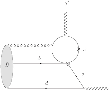
Figure 2: The correlation function used to calculate the $B\to K^{(*)}$ matrix element of the soft-gluon emission from the charm loop. The oval denotes the $B$-meson quark-antiquark-gluon distribution amplitudes. The $c$-quark loop with the emitted gluon generates the nonlocal effective operator $\widetilde{O}_{\mu}$. The cross indicates the point of gluon emission in the second diagram.

In the adopted approximation, the amplitude ${\cal A}$ is factorized:

$${\cal A}(q^{2})=\frac{9}{32\pi^{2}}~{}g(m_{c}^{2},q^{2})f^{+}_{BK}(q^{2})\,,$$ (32)

if one uses (9) and the standard definition of the $B\to K$ form factor:

$$\langle K(p)|\bar{s}_{L}\gamma_{\rho}b_{L}|B(p+q)\rangle=f^{+}_{BK}(q^{2})p_{\rho}+...$$ (33)

Our main task is to calculate the amplitude $\tilde{\cal A}$ determining the soft-gluon emission from the charm-loop. To this end, we employ LCSR with the $B$-meson DA’s and, following [10, 11], introduce the correlation function:

$${\cal F}^{(B\to K)}_{\nu\mu}(p,q)=i\int d^{4}ye^{ip\cdot y}\langle 0|T\{j_{\nu}^{K}(y)\widetilde{{\cal O}}_{\mu}(q)\}|B(p+q)\rangle\,,$$ (34)

where $j_{\nu}^{K}=\bar{d}\gamma_{\nu}\gamma_{5}s$ is the $K$-meson interpolating current and $B$ meson is taken on shell, as a HQET state: $|B(p+q)\rangle\simeq|B(v)\rangle$. Inserting the full set of states with the kaon quantum numbers between the current $j_{\nu}^{K}$ and $\widetilde{{\cal O}}_{\mu}$ in (34) we obtain the hadronic dispersion relation:

$${\cal F}^{(B\to K)}_{\nu\mu}(p,q)={if_{K}p_{\nu}\over m_{K}^{2}-p^{2}}[(p\cdot q)q_{\mu}-q^{2}p_{\mu}]\tilde{{\cal A}}(q^{2})+\int_{s_{h}}^{\infty}ds\,\,{\tilde{\rho}_{\nu\mu}(s,q^{2})\over s-p^{2}}\,,$$ (35)

where $f_{K}$ is the kaon decay constant defined as $\langle 0|\bar{d}\gamma_{\nu}\gamma_{5}s|K(p)\rangle=if_{K}p_{\nu}$ and the spectral density $\tilde{\rho}_{\nu\mu}(s,q^{2})$ accumulates excited and continuum states with the kaon quantum numbers, located above the threshold $s_{h}$.

Two comments are in order. First, in the approach we are using, hadronic matrix elements are related to the correlation function via dispersion relation. Hence, the “full” hadronic matrix element of $B\to K$ transition with the soft-gluon emission enters the residue of the kaon pole in (35). In other words, although we have chosen a particular correlation function with $B$-meson DA’s, there is no need to add a contribution where a soft gluon emitted from the charm loop enters the final-state kaon “wave function”. Secondly, at very large timelike $p^{2}$ there are also “parasitic” charm-anticharm states contributing to the hadronic spectral density in (35), but they are heavily suppressed after the Borel transformation in $p^{2}$. This circumstance allows one to avoid introducing an auxiliary 4-momentum in the effective-operator vertex, as suggested in [24].

In [11] the form factor $f^{+}_{BK}(q^{2})$ was calculated from the correlation function similar to (34), where, instead of the complicated effective operator, the $b\to s$, vector current was inserted. LCSR was obtained including the contributions of two-particle (quark-antiquark) and three-particle (quark-antiquark-gluon) $B$-meson DA’s. Here the leading-order diagrams shown in Fig. 2 involve only the three-particle DA’s of $B$ meson. We calculate these diagrams contracting the $s$-quark fields. The result reduces to the vacuum-to-$B$ matrix element of the $\bar{d}Gb$ nonlocal operator. It is decomposed in HQET in four three-particle $B$-meson DA’s [26]:

$$\langle 0|\bar{d}_{\alpha}(y)\delta[\omega-{(in_{+}{\cal D})\over 2}]G_{\sigma\tau}(0)b_{\beta}(0)|\bar{B}(v)\rangle$$ (36)

$$={f_{B}m_{B}\over 2}\int_{0}^{\infty}d\lambda\,e^{-i\lambda y\cdot v}\bigg{[}(1+\not v)\bigg{\{}(v_{\sigma}\gamma_{\tau}-v_{\tau}\gamma_{\sigma})\big{[}\Psi_{A}(\lambda,2\omega)-\Psi_{V}(\lambda,2\omega)\big{]}$$

$$-i\sigma_{\sigma\tau}\Psi_{V}(\lambda,2\omega)-{y_{\sigma}v_{\tau}-y_{\tau}v_{\sigma}\over v\cdot y}X_{A}(\lambda,2\omega)+{y_{\sigma}\gamma_{\tau}-y_{\tau}\gamma_{\sigma}\over v\cdot y}Y_{A}(\lambda,2\omega)\bigg{\}}\gamma_{5}\bigg{]}_{\beta\alpha}\,,$$

where $f_{B}$ and $m_{B}$ are the $B$-meson decay constant and mass, respectively. Further details can be found in [11].

Equating the correlation function $\cal{F}_{\nu\mu}$, written in terms of the $B$-meson DA’s, to its hadronic representation (35), we perform the Borel transformation in the variable $p^{2}$ and employ quark-hadron duality in the kaon channel to approximate the integral over the spectral density $\tilde{\rho}_{\nu\mu}$, introducing the effective duality threshold $s_{0}^{K}$. The resulting LCSR for the nonfactorizable $B\to K$ hadronic matrix element of the charm-loop effect reads:

$$\tilde{{\cal A}}(q^{2})=-\frac{f_{B}m_{B}}{8\pi^{2}f_{K}(m_{B}^{2}-m_{K}^{2}-q^{2})}\int\limits_{0}^{\sigma_{0}}d\sigma\int\limits_{0}^{\infty}\!\!d\omega\int\limits_{0}^{1}\!\!du\int\limits_{0}^{1}\!\!dt\,\exp\Big{(}\frac{m_{K}^{2}-\sigma m_{B}^{2}}{M^{2}}\Big{)}$$

$$\times\!\frac{1}{m_{c}^{2}-t(1-t)(q^{2}-2m_{B}u\,\omega)}\Bigg{[}C^{(\Psi_{V})}(q^{2},u,\sigma,\omega,t)\Psi_{V}(m_{B}\sigma,2\omega)$$

$$+C^{(\Psi_{AV})}(q^{2},u,\sigma,\omega,t)\big{[}\Psi_{V}(m_{B}\sigma,2\omega)-\Psi_{A}(m_{B}\sigma,2\omega)\big{]}$$ (37)

$$+C^{(X_{A})}(q^{2},u,\sigma,\omega,t)\bar{X}_{A}(m_{B}\sigma,2\omega)-\frac{d}{d\sigma}\big{[}\widetilde{C}^{(X_{A})}(q^{2},u,\sigma,\omega,t)\bar{X}_{A}(m_{B}\sigma,2\omega)\big{]}$$

$$+C^{(Y_{A})}(q^{2},u,\sigma,\omega,t)\bar{Y}_{A}(m_{B}\sigma,2\omega)-\frac{d}{d\sigma}\big{[}\widetilde{C}^{(Y_{A})}(q^{2},u,\sigma,\omega,t)\bar{Y}_{A}(m_{B}\sigma,2\omega)\big{]}\Bigg{]},$$

where $M^{2}$ is the Borel parameter, $\sigma_{0}\simeq s^{K}_{0}/m_{B}^{2}$ (up to small corrections),

$$\bar{X}_{A}(\lambda,\omega)=\int_{0}^{\lambda}d\tau X_{A}(\tau,\omega),\qquad\bar{Y}_{A}(\lambda,\omega)=\int_{0}^{\lambda}d\tau Y_{A}(\tau,\omega).$$ (38)

and the coefficients $C^{(...)}$ and $\widetilde{C}^{(...)}$ are collected in Appendix D. The sum rule is presented in (4) in a simplified form, omitting the $s$-quark mass and small $O(1/m_{B}^{2})$ corrections. In the numerical analysis the complete expression is used.

Note that the spectral density of the correlation function (34) in the variable $p^{2}$, in addition to the $s$-quark pole, contains also “parasitic” contributions which correspond to putting simultaneously on-shell the $s$-quark and the $\bar{c}c$-quark lines in the diagram of Fig. 2. After Borel transformation these terms are suppressed by $\sim\exp(-4m_{c}^{2}/M^{2})$ and we neglect them. As noted above, the corresponding hadronic states are also neglected in the dispersion relation.

In order to assess the accuracy of using the nonlocal effective operator $\tilde{\cal O}_{\mu}$ in the correlation function we derived the LCSR in an alternative way, inserting the operator $C_{1}O_{1}+C_{2}O_{2}$ and the c-quark e.m. current directly in the correlation function. As a result we obtain a more complicated expression for LCSR, which differs from (4) only by terms suppressed by inverse powers of $m_{c}$ and/or $m_{B}$, and yields numerically very close results for the amplitude $\tilde{{\cal A}}$. Finally, the local OPE limit of LCSR (4) was also investigated, that is, when the soft-gluon momentum is neglected. This limit literally corresponds to putting $\omega\to 0$ in the coefficients $C^{(...)}$ and in the denominator of (4). The numerical influence of this approximation will be discussed in the next section.

Turning to the calculation of the $B\to K^{*}$ transition matrix element defined in (4) we decompose it into the three kinematical structures:

$${\cal H}_{\mu}^{(B\to K^{*})}(p,q) = \left(C_{2}+\frac{C_{1}}{3}\right)\langle K^{*}(p)|{\cal O}_{\mu}(q)|B(p+q)\rangle+2C_{1}\langle K^{*}(p)|\widetilde{{\cal O}}_{\mu}(q)|B(p+q)\rangle$$ (39)

$$= \epsilon_{\mu\alpha\beta\gamma}\epsilon^{\ast\alpha}q^{\beta}p^{\gamma}{\cal H}_{1}(q^{2})+i[(m_{B}^{2}-m^{2}_{K^{\ast}})\epsilon^{\ast}_{\mu}-(\epsilon^{\ast}\!\cdot q)(2p+q)_{\mu}]{\cal H}_{2}(q^{2})$$

$$+i(\epsilon^{\ast}\!\cdot q)\bigg{[}q_{\mu}-{q^{2}\over m_{B}^{2}-m^{2}_{K^{\ast}}}(2p+q)_{\mu}\bigg{]}{\cal H}_{3}(q^{2})\,,$$

where $\epsilon$ is the polarization vector of the $K^{*}$-meson.

The invariant amplitudes in the above decomposition contain factorizable and nonfactorizable parts stemming from the matrix elements of ${\cal O}_{\mu}$ and $\widetilde{{\cal O}}_{\mu}$, respectively:

$${\cal H}_{i}^{(B\to K^{*})}(q^{2})=\left(C_{2}+\frac{C_{1}}{3}\right){\cal V}_{i}(q^{2})+2C_{1}\widetilde{{\cal V}}_{i}(q^{2})\,~{}~{}~{}(i=1,2,3).$$ (40)

The three factorizable amplitudes ${\cal V}_{i}$ are easily obtained if one uses (9) and the standard definition of $B\to K^{*}$ vector and axial-vector form factors:

$$2\langle K^{\ast}(p)|\bar{s}_{L}\gamma_{\rho}b_{L}|B(p+q)\rangle=\epsilon_{\rho\alpha\beta\gamma}\epsilon^{*\alpha}q^{\beta}p^{\gamma}\dfrac{2V^{BK^{*}}(q^{2})}{m_{B}+m_{K^{*}}}$$

$$-i\epsilon_{\rho}^{*}(m_{B}+m_{K^{*}})A_{1}^{BK^{*}}(q^{2})+i(2p+q)_{\rho}(\epsilon^{*}q)\dfrac{A_{2}^{BK^{*}}(q^{2})}{m_{B}+m_{K^{*}}}+\ldots\,,$$ (41)

where the form factors multiplying $q_{\rho}$ do not contribute and are indicated by ellipses. We have:

$${\cal V}_{1}(q^{2}) = -{9q^{2}\over 32\pi^{2}(m_{B}+m_{K^{\ast}})}g(m_{c}^{2},q^{2})V^{BK^{\ast}}(q^{2})\,,$$

$${\cal V}_{2}(q^{2}) = {9q^{2}\over 64\pi^{2}(m_{B}-m_{K^{\ast}})}g(m_{c}^{2},q^{2})A_{1}^{BK^{\ast}}(q^{2})\,,$$

$${\cal V}_{3}(q^{2}) = \frac{9(m_{B}^{2}-m_{K^{\ast}}^{2})}{64\pi^{2}}g(m_{c}^{2},q^{2})\Bigg{(}\frac{A_{2}^{BK^{\ast}}(q^{2})}{m_{B}+m_{K^{\ast}}}-\frac{A_{1}^{BK^{\ast}}(q^{2})}{m_{B}-m_{K^{\ast}}}\Bigg{)}\,.$$ (42)

To calculate the nonfactorizable amplitudes $\widetilde{{\cal V}}_{i}(q^{2})$ ($i=1,2,3$), describing the soft-gluon emission we again resort to the LCSR method, introducing the correlation function

$${\cal F}^{(B\to K^{*})}_{\nu\mu}(p,q)=i\int d^{4}y\,e^{ip\cdot y}\langle 0|T\{j_{\nu}^{K^{\ast}}(y)\widetilde{{\cal O}}_{\mu}(q)\}|B(p+q)\rangle\,,$$ (43)

where $j_{\nu}^{K^{\ast}}=\bar{d}\gamma_{\nu}s$ is the interpolating current for the $K^{\ast}$ meson. The hadronic dispersion relation for this correlation function reads:

$${\cal F}^{(B\to K^{*})}_{\nu\mu}(p,q)=\frac{f_{K^{*}}m_{K^{*}}\overline{\epsilon_{\nu}\langle K^{*}(p)|}\widetilde{{\cal O}}_{\mu}(q)|B(p+q)\rangle}{m^{2}_{K^{*}}-p^{2}}+\int_{s_{h}^{*}}^{\infty}ds\,\,{\widetilde{\rho}\,^{*}_{\nu\mu}(s,q^{2})\over s-p^{2}}\,,$$ (44)

where $f_{K^{*}}$ is the $K^{*}$ decay constant defined as $\langle 0|j_{\nu}^{K^{\ast}}|K^{*}(p)\rangle=\epsilon_{\nu}m_{K^{*}}f_{K^{*}}$ and the overline denotes the average over $K^{*}$ polarizations. We neglect the total width of $K^{*}$. This approximation can in principle be avoided by introducing a Breit-Wigner type parameterization for this resonance. Excited and continuum states with $K^{*}$ quantum numbers above the threshold $s_{h}^{*}$ contribute to the spectral density $\tilde{\rho}^{*}_{\nu\mu}(s,q^{2})$. The latter is approximated using quark-hadron duality and introducing an effective threshold $s_{0}^{K^{*}}$.

Furthermore, the $K^{*}$ contribution in (44) is written in terms of invariant amplitudes:

$$\big{[}{\cal F}^{(B\to K^{*})}_{\nu\mu}(p,q)\big{]}^{K^{*}}\!\!\!\! = \!\!\!\!\,\,\frac{if_{K^{*}}m_{K^{*}}}{m_{K^{*2}}-p^{2}}\Bigg{[}i\epsilon_{\mu\nu\beta\gamma}q^{\beta}p^{\gamma}\tilde{\cal V}_{1}(q^{2})-(m_{B}^{2}-m^{2}_{K^{\ast}})g_{\mu\nu}\tilde{\cal V}_{2}(q^{2})$$ (45)

$$+ \!\!\!\!\,\,q_{\mu}q_{\nu}\bigg{(}\tilde{\cal V}_{2}(q^{2})-(1-\frac{q^{2}}{m_{B}^{2}-m_{K^{*2}}})\tilde{\cal V}_{3}(q^{2})\bigg{)}\Bigg{]}+...\,,$$

where we only show the kinematical structures that have been used in our analysis. Applying the same decomposition to the OPE result for the correlation function ${\cal F}^{*}_{\nu\mu}$ we obtain three sum-rule relations which are then used to calculate the hadronic matrix elements $\tilde{{\cal V}}_{1,2,3}(q^{2})$. The derivation of these LCSR in terms of $B$-meson DA’s is very similar to the one described for $B\to K$ case. Indeed, the only difference between the two correlation functions (34) and (43) is in the quantum numbers of the $s$-quark current. The resulting LCSR for $\tilde{{\cal V}}_{i}(q^{2})$ has the same structure as (4), only the coefficients multiplying the $B$-meson DA’s and the overall normalization factors are different. In order not to overload this paper, we do not present these expressions here.

5 Numerical analysis

We use LCSR with $B$ meson DA’s to evaluate not only the nonfactorizable amplitudes $\widetilde{{\cal A}}$ and $\widetilde{{\cal V}_{i}}$ but also the $B\to K$ and $B\to K^{*}$ form factors entering the factorizable parts ${\cal A}$ and ${\cal V}_{i}$ given by (32) and (42). The sum rules for these form factors and their input are taken from [11], hence we use the same input for the new LCSR obtained in the previous section. In particular, for the three-particle $B$-meson DA’s the model suggested in [11] is taken:

$$\Psi_{A}(\lambda,\omega) = \Psi_{V}(\lambda,\omega)={\lambda_{E}^{2}\over 6\omega_{0}^{4}}\omega^{2}e^{-(\lambda+\omega)/\omega_{0}}\,,$$

$$X_{A}(\lambda,\omega) = {\lambda_{E}^{2}\over 6\omega_{0}^{4}}\omega(2\lambda-\omega)e^{-(\lambda+\omega)/\omega_{0}}\,,$$

$$Y_{A}(\lambda,\omega) = -{\lambda_{E}^{2}\over 24\omega_{0}^{4}}\omega(7\omega_{0}-13\lambda+3\omega)e^{-(\lambda+\omega)/\omega_{0}}\,.$$ (46)

In this model the parameter $\omega_{0}$ is equal to the inverse moment $\lambda_{B}$ of the $B$ meson two-particle DA $\phi^{B}_{+}$ and the normalization constant of the three-particle DA’s is $\lambda^{2}_{E}=3/2\lambda_{B}^{2}$. For the inverse moment we use the interval obtained in [27] from QCD sum rule in HQET: $\lambda_{B}(1{\rm GeV})=460\pm 110\,{\rm MeV}\,$. The scale-dependence of this parameter is neglected. To be consistent with the $O(\alpha_{s})$ accuracy of $\lambda_{B}$, the $B$-meson decay constant $f_{B}=180\pm 30~{}~{}{\rm MeV}$ obtained from the two-point QCD sum rules in $O(\alpha_{s})$ is used. Furthermore, the decay constants and threshold parameters of $K$ and $K^{\ast}$ mesons are taken the same as in [11]:

$$f_{K} = 159.8\pm 1.4\pm 0.44\,{\rm MeV}\,,\qquad f_{K^{\ast}}=217\pm 5\,{\rm MeV}\,,$$

$$s_{0}^{K} = 1.05\,{\rm GeV^{2}}\,,\qquad\hskip 56.9055pts_{0}^{K^{\ast}}=1.7\,{\rm GeV^{2}}\,.$$ (47)

For the Borel parameter interval in LCSR we use is $M^{2}=1.0\pm 0.25~{}{\rm GeV^{2}}$, slightly narrower than the interval in [11].

In addition, we need the $c$-quark mass value. Since we are dealing with virtual $\bar{c}c$-quark loops, it is natural to employ the $\overline{MS}$ mass, assuming that the normalization scale is about $2\bar{m}_{c}$. As a default value, we take $\bar{m}_{c}(2\bar{m}_{c})=1.05~{}{\rm GeV}$, rescaled from the central value of $\bar{m}_{c}$ obtained from charmonium sum rule in [28]. To assess the related uncertainty we allow the normalization scale to change between $2m_{c}$ and $m_{c}$, shifting the $c$-quark mass to $m_{c}(\bar{m}_{c})=1.30~{}\mbox{GeV}$. Finally, $m_{s}(\rm 2\,GeV)=98\pm 16~{}{\rm MeV}$ is adopted (the average of nonlattice determinations [29]).

Figure 3: The nonfactorizable $B\to K$ amplitude $\widetilde{{\cal A}}(q^{2})$ of the nonlocal effective operator $\widetilde{O}_{\mu}$ (solid) and its local limit (dash-dotted), plotted as a function of $q^{2}$, together with the factorizable amplitude ${\cal A}(q^{2})$ (dashed). The soft-gluon contributions are rescaled with a factor of 10.

In Fig. 3 our numerical results for the $q^{2}$-dependence of the dimensionless hadronic amplitudes ${\cal A}(q^{2})$ and $\widetilde{{\cal A}}(q^{2})$ are displayed for the central values of the input. For convenience, we normalize both amplitudes to ${\cal A}(0)=7.3\times 10^{-3}$. The nonfactorizable amplitude is about a few percent of the factorizable one and has the opposite sign. Note that both ${\cal A}(q^{2})$ and $\widetilde{{\cal A}}(q^{2})$ develop imaginary parts above $4m_{c}^{2}$. In the same figure we plot the nonfactorizable amplitude $\widetilde{{\cal A}}(q^{2})$ obtained in the local OPE limit. In this case, the nonfactorizable effect changes substantially and diverges approaching to $q^{2}=4m_{c}^{2}$. We come to an important conclusion that the effective resummation the local operators in the framework of the light-cone OPE “softens” the gluon correction to the charm loop.

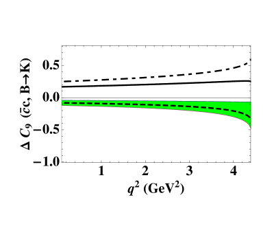
Figure 4: The charm-loop effect in $B\to K\ell^{+}\ell^{-}$ expressed as a correction to the Wilson coefficient $C_{9}$ (solid), including the nonfactorizable soft-gluon contribution (dashed) with the shaded region indicating the estimated uncertainty and the factorizable contribution (dash-dotted).

In the decay amplitude the soft-gluon contribution to the charm-loop effect gets enhanced considerably with respect to the factorizable one by the ratio of the Wilson coefficients $2C_{1}/(C_{2}+C_{1}/3)\gg 1$. Not surprisingly then, the proportion of the two contributions depends on the normalization scale of the Wilson coefficients. The scale can be fixed more accurately when the perturbative gluon corrections in the hadronic matrix elements are taken into account, which is beyond our approximation.

Figure 5: The same as in Fig. 4 for $\bar{B}_{0}\to\bar{K^{\ast}}l^{+}l^{-}$. The results for the correction to the amplitude ${\cal M}_{2}$ are almost indistinguishable from the ones for ${\cal M}_{1}$ shown in the upper panel.

For the numerical estimates we use the values of the Wilson coefficients given in Appendix A. They are calculated in leading log approximation at $\mu=m_{b}$, allowing the scale to vary between $0.5m_{b}$ and $1.5m_{b}$. Note that in our calculation the $b$-quark mass value only enters the effective Hamiltonian. We adopt the $\overline{MS}$ value extracted from the bottomonium sum rules in [28] $\bar{m}_{b}(\bar{m}_{b})=4.164\pm 0.025~{}{\rm GeV}$ (conservatively doubling the error).

It is convenient to express the charm-loop contribution to the $B\to K\ell^{+}\ell^{-}$ amplitude in a form of a (process- and $q^{2}$-dependent) correction to the Wilson coefficient $C_{9}$:

$$C_{9}\to C_{9}+\Delta C_{9}^{(\bar{c}c,B\to K)}(q^{2})\,.$$ (48)

Substituting (30),(31) and (32) to (3) and comparing the result with the contribution of $O_{9}$ to the $B\to K\ell^{+}\ell^{-}$ amplitude given in Appendix A, we obtain:

$$\Delta C_{9}^{(\bar{c}c,B\to K)}(q^{2}) = \frac{32\pi^{2}}{3}\frac{{\cal H}^{(B\to K)}(q^{2})}{f^{+}_{BK}(q^{2})}$$ (49)

$$= \left(C_{1}+3C_{2}\right)g(m_{c}^{2},q^{2})+2C_{1}\widetilde{g}^{(\bar{c}c,B\to K)}(q^{2})\,,$$

where the function

$$\widetilde{g}^{(\bar{c}c,B\to K)}(q^{2})=\frac{32\pi^{2}}{3}\frac{\tilde{{\cal A}}(q^{2})}{f^{+}_{BK}(q^{2})}$$ (50)

determines the new soft-gluon nonfactorizable part of $\Delta C_{9}^{(\bar{c}c,B\to K)}$ and represents our main result. Here only the ratio of the calculated hadronic matrix elements enter and they both are calculated within one and the same LCSR approach. The correction $\Delta C_{9}^{(\bar{c}c,B\to K)}$ and its factorizable and nonfactorizable parts are plotted in Fig. 4 where the uncertainties stemming from our calculation of $\widetilde{g}^{(\bar{c}c,B\to K)}(q^{2})$ are indicated. We vary all input parameters within their adopted intervals and add individual variations in the quadrature. In Table 1 we display the value and the estimated uncertainties of $\widetilde{g}^{(\bar{c}c,B\to K)}$ at $q^{2}=1$ GeV², except the variation due to uncertainty of $m_{s}$ which is negligibly small.

Table 1: The functions determining the soft-gluon correction to $C_{9}$, calculated from LCSR, central values at $q^{2}=1\,\rm GeV^{2}$, and the uncertainties $\Delta_{a}$ caused by the variations of the input parameters ($\delta_{m_{c}}=+0.25\,{\rm GeV}$, $\delta_{M^{2}}=^{+0.25}_{-0.25}\,{\rm GeV}$, $\delta_{\lambda_{B}}=^{+110}_{-110}\,{\rm MeV}$).

function	$\tilde{g}^{(\bar{c}c,B\to K)}$	$\tilde{g}^{(\bar{c}c,B\to K^{\ast},M_{1})}$	$\tilde{g}^{(\bar{c}c,B\to K^{\ast},M_{2})}$	$\tilde{g}^{(\bar{c}c,B\to K^{\ast},M_{3})}$
centr.value	$-0.041$	$0.26$	$0.27$	$0.46$
$\Delta_{m_{c}}$	$+0.014$	-0.08	-0.09	-0.15
$\Delta_{M^{2}}$	${}^{+0.00}_{-0.001}$	${}^{-0.04}_{+0.07}$	${}^{-0.04}_{+0.08}$	${}^{-0.07}_{+0.12}$
$\Delta_{\lambda_{B}}$	${}^{-0.016}_{+0.017}$	${}^{+0.30}_{-0.17}$	${}^{+0.36}_{-0.18}$	${}^{+0.75}_{-0.33}$
$\Delta_{tot}$	${}^{+0.022}_{-0.016}$	${}^{+0.31}_{-0.19}$	${}^{+0.37}_{-0.21}$	${}^{+0.76}_{-0.37}$

Note that substantial uncertainties are caused by the shift of $m_{c}$ and rather broad interval of the inverse moment $\lambda_{B}$ of the $B$-meson DA.

To parameterize the charm-loop effect for the $B\to K^{*}\ell^{+}\ell^{-}$ decay amplitude we use its decomposition in the three invariant amplitudes ${\cal M}_{i}$ presented in Appendix B and the corresponding decompositions (39) and (40). As a result the terms proportional to $C_{9}$ in the amplitudes ${\cal M}_{1,2,3}$, have to be modified in the following way:

$$\Delta C_{9}^{(\bar{c}c,B\to K^{*},\,{\cal M}_{i})}(q^{2})=\left(C_{1}+3C_{2}\right)g(m_{c}^{2},q^{2})+2C_{1}\widetilde{g}\,^{(\bar{c}c,B\to K^{*},\,{\cal M}_{i})}(q^{2})\,,$$ (51)

where, respectively,

$$\widetilde{g}\,^{(\bar{c}c,B\to K^{*},\,{\cal M}_{1})}(q^{2}) = -{32\pi^{2}\over 3}{(m_{B}+m_{K^{*}})\widetilde{{\cal V}}_{1}(q^{2})\over q^{2}V^{BK^{*}}(q^{2})}\,,$$

$$\widetilde{g}\,^{(\bar{c}c,B\to K^{*},\,{\cal M}_{2})}(q^{2}) = {64\pi^{2}\over 3}{(m_{B}-m_{K^{\ast})}\over q^{2}}\frac{\widetilde{{\cal V}}_{2}(q^{2})}{A_{1}^{BK^{*}}(q^{2})}\,,$$

$$\widetilde{g}\,^{(\bar{c}c,B\to K^{*},\,{\cal M}_{3})}(q^{2}) = {64\pi^{2}\over 3}\bigg{[}{(m_{B}+m_{K}^{*})\widetilde{{\cal V}}_{2}(q^{2})\over q^{2}A_{2}^{BK^{*}}(q^{2})}$$ (52)

$$+{\widetilde{{\cal V}}_{3}(q^{2})\over(m_{B}-m_{K^{\ast}})A_{2}^{BK^{*}}(q^{2})}\bigg{]}\,.$$

Note that the nonfactorizable contributions to $\Delta C_{9}^{(\bar{c}c,B\to K^{*},\,{\cal M}_{i})}$ are enhanced at small $q^{2}\geq 4m_{\ell}^{2}$ with respect to the factorizable ones due to the virtual photon propagator (the same enhancement as in the $C_{7}$ contribution). Our predictions for $\Delta C_{9}^{(\bar{c}c,B\to K^{*},\,{\cal M}_{i})}(q^{2})$ are plotted in Fig. 5. In Table 1 we present a sample of numerical results and estimated uncertainties for $\widetilde{g}\,^{(\bar{c}c,B\to K^{*},\,{\cal M}_{i})}(1\mbox{GeV}^{2})$. The charm-loop effect and its soft-gluon part in $B\to K^{*}\ell^{+}\ell^{-}$ transitions is predicted to be considerably larger than in $B\to K\ell^{+}\ell^{-}$, having also a larger uncertainty. Moreover, the nonfactorizable contributions in $B\to K^{*}$ have the same sign as the factorizable ones, which leads to an additional enhancement of the charm-loop effect.

We come to an important conclusion that the calculated charm-loop correction
$\Delta C_{9}^{(\bar{c}c,B\to K)}(q^{2})$ in $B\to K\ell^{+}\ell^{-}$ remains small, not exceeding (within uncertainties) $\sim 5\%$ of the $C_{9}$ value at $0<q^{2}<$ 4.0 GeV². In $B\to K^{*}\ell^{+}\ell^{-}$ the same ratio may reach (adding up the estimated uncertainties) as much as 20% of $C_{9}$ at $1.0<q^{2}<4.0$ GeV² and is inflated at smaller $q^{2}$. In both decays, especially in $B\to K^{*}\ell^{+}\ell^{-}$, the nonfactorizable soft-gluon part of $\Delta C_{9}$ plays a decisive role. At $q^{2}\geq 4.0$ GeV² where OPE for the charm-loop effect starts to diverge we will use a phenomenological ansatz for $\Delta C_{9}^{(\bar{c}c,B\to K^{*},\,{\cal M}_{i})}(q^{2})$ presented below, in Sect. 7.

6 Charm-loop effect in $B\to K^{*}\gamma$

We are in a position to predict the charm-loop effect also in $B\to K^{*}\gamma$ which is simply a by-product of our calculation for $B\to K^{*}\ell^{+}\ell^{-}$ at $q^{2}=0$. Importantly, in this case only the nonfactorizable soft-gluon emission contributes. With the effective resummation of this effect, our result goes beyond the estimates in [6] and [7] where the matrix elements of the local quark-gluon operator were calculated.

To specify the normalization, in Appendix B we present the dominant contribution to the $B\to K^{\ast}\gamma$ amplitude, due to the operator $O_{7}$. The charm-loop effect is included in this amplitude by the following additions to the Wilson coefficient $C_{7}^{eff}$ multiplying the first and second kinemetical structures in this amplitude, respectively:

$$C_{7}^{eff}\to C_{7}^{eff}+[\Delta C_{7}^{(\bar{c}c,B\to K^{*}\gamma)}]_{1,2}\,,$$ (53)

where

$$~{}~{}[\Delta C_{7}^{(\bar{c}c,B\to K^{*}\gamma)}]_{1}=\frac{32\pi^{2}}{3}\frac{C_{1}\tilde{\mathcal{V}}_{1}(0)}{(m_{b}+m_{s})T_{1}^{BK^{\ast}}(0)}\,,$$

$$~{}~{}[\Delta C_{7}^{(\bar{c}c,B\to K^{*}\gamma)}]_{2}=-\frac{64\pi^{2}}{3}\frac{C_{1}\tilde{\mathcal{V}}_{2}(0)}{(m_{b}-m_{s})T_{1}^{BK^{\ast}}(0)}\,.$$ (54)

The numerical analysis reveals that the corrections to both amplitudes are approximately equal:

$$\big{[}\Delta C_{7}^{(\bar{c}c,B\to K^{*}\gamma)}\big{]}_{1}\simeq\big{[}\Delta C_{7}^{(\bar{c}c,B\to K^{*}\gamma)}\big{]}_{2}=(-1.2^{+0.9}_{-1.6})\times 10^{-2}\,,$$ (55)

amounting up to 8 % of the coefficient $C_{7}^{eff}$. Our estimate yields larger magnitude (also with larger uncertainty) than predicted in [7] where the local OPE and LCSR with $K^{*}$-meson DA’s were used. Normalizing the hadronic matrix elements calculated in [7] as in (54) and using their input, we obtain

$$~{}~{}[\Delta C_{7}^{(\bar{c}c,B\to K^{*}\gamma)}]_{1}^{BZ}=(-0.39\pm 0.3)\times 10^{-2}\,,$$

$$~{}~{}[\Delta C_{7}^{(\bar{c}c,B\to K^{*}\gamma)}]_{2}^{BZ}=(-0.65\pm 0.57)\times 10^{-2}\,.$$ (56)

Note that if we also use the local OPE limit, both amplitudes in (55) have about 40% larger magnitudes, approaching the estimates obtained from the three-point QCD sum rules in [6].

7 Accessing large $q^{2}$ with dispersion relation

Returning to the hadronic matrix element (4) we use its analyticity in the variable $q^{2}$, expressed in the form of dispersion relation. Considering first the $B\to K$ case, we obtain the corresponding spectral density, inserting in (4) the full set of hadronic states with the quantum numbers of $J/\psi$ between the $c$-quark current and the four-quark operator. Introducing the hadronic matrix elements

$$\langle 0|\bar{c}\gamma^{\rho}c|\psi(q)\rangle=\epsilon_{\psi}^{\rho}m_{\psi}f_{\psi}\,,$$ (57)

$$\langle K(p)\psi(q)|C_{1}O_{1}+C_{2}O_{2}|B(p+q)\rangle=(\epsilon_{\psi}^{*}\cdot p)m_{\psi}A_{B\psi K}\,,$$ (58)

where $\psi=J/\psi,\psi(2S)$ and $\epsilon_{\psi}$ is the polarization vector, we obtain the dispersion relation for the invariant amplitude:

$${\cal H}^{(B\to K)}(q^{2})={\cal H}^{(B\to K)}(0)+q^{2}\Big{[}\sum_{\psi=J/\psi,\psi(2S)}\frac{f_{\psi}A_{B\psi K}}{m_{\psi}^{2}(m_{\psi}^{2}-q^{2}-im_{\psi}\Gamma^{tot}_{\psi})}$$

$$+\int_{4m_{D}^{2}}^{\infty}ds\frac{\rho(s)}{s(s-q^{2}-i\epsilon)}\Big{]}\,,$$ (59)

where $\rho(s)$ is the spectral density of $\psi$-resonances and continuum $c\bar{c}$-states located above the open charm threshold, $s\geq 4m_{D}^{2}$. In (59) we include the small total widths of $J/\psi$ and $\psi(2S)$, but neglect the complex phase everywhere beyond the immediate vicinity of the resonances. One subtraction at $q^{2}=0$ takes into account that the spectral density (12) of the factorizable loop contained in ${\cal H}^{(B\to K)}(q^{2})$ tends to a constant at $s\!\to\!\infty$. Note that the soft-gluon contribution has a convergent dispersion integral as follows from the spectral density (24). The parameters of $\psi$-poles in (59) are presented in Appendix C, including the decay constants $f_{\psi}$ and the absolute values of the invariant amplitudes $A_{B\psi K}$ calculated from the measured $B\to\psi K$ widths.

It is well known that the naive factorization approximation for these amplitudes: $A_{B\psi K}=(C_{2}+C_{1}/3)f_{\psi}f^{+}_{BK}(m_{\psi}^{2})$ is not consistent with the experimental data, indicating sizeable nonfactorizable corrections. Moreover, both amplitudes $A_{BJ/\psi K}$ and $A_{B\psi(2S)K}$ are expected to have complex phases generated by the strong final-state interactions in these nonleptonic decays . Note that the diagrams with perturbative gluons (e.g., the $O(\alpha_{s})$ diagram in Fig. 1c,d) generate complex phases in ${\cal H^{B\to K}}(q^{2})$. One can speculate that they are dual to the final-state interaction phases in $A_{B\psi K}$, in a certain analogy with the QCD factorization approach [30]. The diagrams with perturbative gluons are not included in our calculation of ${\cal H^{B\to K}}(q^{2})$, hence we also neglect complex phases in the hadronic part of the dispersion relation. On the other hand, we notice that after taking the soft-gluon emission into account, the amplitude ${\cal H}^{(B\to K)}(q^{2})$, is not positive-definite anymore. Indeed, the nonfactorizable part $\tilde{{\cal A}}$ of this amplitude obtained from LCSR has a negative sign with respect to the factorizable part ${\cal A}$. Therefore, we relax the positivity condition for the spectral density in (59), allowing, e.g., different signs between the residues of $\psi$-poles . This makes (59) essentially different from the dispersion relations used earlier in [13, 15].

The most complicated part of the dispersion relation (59) is the spectral density $\rho(s)$ above the open-charm threshold. It includes an interplay of broad charmonium resonances and continuum states. Since we are working beyond the factorization approximation, we do not attempt to describe this spectral function as a sum over higher $\psi$ resonances and a tail determined by quark-hadron duality with the $c$-quark loop as in [13]. In future $\rho(s)$ can be partially determined and/or constrained up to $s=(m_{B}-m_{K})^{2}$, employing the experimental data on the nonleptonic decays $B\to\psi K$, ($\psi=\psi(3770),...$) and $B\to\bar{D}DK,\bar{D}^{*}DK,...$. Note also, that at $q^{2}$ approaching the upper threshold $(m_{B}-m_{K})^{2}$, the dispersion relation will also be influenced by the singularities in $\rho(s)$ related to the intermediate $b\bar{s}$ states. Hence we refrain from using the quark-hadron duality approximation for the integral over $\rho(s)$ in (59). The simplest possible choice is to model this integral by an effective pole:

$$\int_{4m_{D}^{2}}^{\infty}ds\frac{\rho(s)}{s(s-q^{2})}\simeq\frac{a^{(B\to K)}}{m_{*}^{2}-q^{2}}\,.$$ (60)

The next step is to match the dispersion relation to the function ${\cal H}^{(B\to K)}(q^{2})$ obtained from OPE and LCSR at $q^{2}\ll 4m_{c}^{2}$. More specifically, we use as an input the l.h.s. of (59) calculated at $-4m_{c}^{2}\leq q^{2}\leq 2$ GeV², so that the subtraction constant ${\cal H}^{B\to K}(0)$ is also determined. Provided the absolute values of $\psi$-poles in (59) are fixed by experimental data [31], this matching allows one to fit the parameters of the effective pole. Importantly, the fit clearly favours a negative relative sign of $J/\psi$ and $\psi(2S)$ contributions, and yields for the central values of the input

$$m_{*}=4.06\mbox{ GeV},~{}~{}a^{(B\to K)}=0.06\times 10^{-3}\,.$$ (61)

The fitted residue of the effective pole turns out to be much smaller than residues of $J/\psi$ and $\psi(2S)$ in (59):

$$\frac{f_{J/\psi}A_{BJ/\psi K}}{m_{J/\psi}^{2}}=1.34\times 10^{-3}\,,~{}~{}\frac{f_{\psi(2S)}A_{B\psi(2S)K}}{m_{\psi(2S)}^{2}}=-0.90\times 10^{-3}.$$ (62)

To investigate the sensitivity of the dispersion relation to the adopted ansatz (60), we also used, as an alternative option, the conformal mapping $q^{2}\to z$ and the $z$-expansion for the integral (60), making use of the fact that it has no singularities at $q^{2}<4m_{D}^{2}$. The resulting dispersion representation for ${\cal H}^{(B\to K)}(q^{2})$ obtained after fitting the coefficients of $z$ expansion numerically differs very little from the one with the effective pole, again favoring the sign pattern as in (62), hence we adopt the latter as a default model.

Finally, we express the dispersion representation of the charm-loop effect in terms of the correction $\Delta C_{9}^{(\bar{c}c,B\to K)}(q^{2})$ defined as in (49). Our numerical prediction is plotted in Fig. 6 up to $q^{2}=m_{\psi(2S)}^{2}$. At $q^{2}\leq 4$ GeV² it coincides with the calculated result shown in Fig. 4. The dashed region in Fig. 6 indicates now all uncertainties, in particular the one which is not related with our calculation and corresponds to the substantial scale-variation of the combination of Wilson coefficients in the factorizable part. Note that at $q^{2}>$ 4 GeV², where we rely on the dispersion relation, it is not possible to split $\Delta C_{9}^{(\bar{c}c,B\to K)}$ into factorizable and nonfactorizable parts. The predicted charm-loop effect in $B\to K\ell^{+}\ell^{-}$ is numerically unimportant at least up to $q^{2}\sim 5-6$ GeV². Within uncertainties it is even consistent with zero, due to possible cancellation of factorizable and nonfactorizable contributions to $\Delta C_{9}(q^{2})^{(\bar{c}c,B\to K)}$ at certain combinations of the input parameters.

Numerically, we find that the correction to $C_{9}$ is well reproduced by the following simple parameterization valid at $0<q^{2}<9$ GeV²

$$\Delta C_{9}^{(\bar{c}c,B\to K)}(q^{2})=\frac{\Delta C_{9}^{(\bar{c}c,B\to K)}(0)+r_{1}^{(B\to K)}\frac{q^{2}}{m_{J/\psi}^{2}}}{1-r_{2}^{(B\to K)}{q^{2}\over m_{J/\psi}^{2}}}\,,$$ (63)

with the calculated

$$\Delta C_{9}^{(\bar{c}c,B\to K)}(0)=0.17^{+0.09}_{-0.18}$$ (64)

and fitted

$$r_{1}=0.01^{+0.13}_{-0.08},~{}~{}r_{2}=1.02^{+0.01}_{-0.01}.$$ (65)

This representation can be used in the phenomenological analysis of $B\to K\ell^{+}\ell^{-}$.

Figure 6: The charm loop contribution to the Wilson coefficient $C_{9}$ for $\bar{B}_{0}\to\bar{K}l^{+}l^{-}$ at $q^{2}$ below the open charm threshold, obtained from the dispersion relation fitted to the OPE result at $q^{2}\ll 4m_{c}^{2}$. The central values are denoted by dashed line, shaded area indicates the estimated uncertainties.

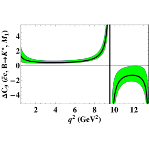
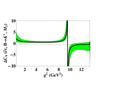
Figure 7: The same as in Fig. 6 for $\bar{B}_{0}\to\bar{K^{\ast}}l^{+}l^{-}$.

The dispersion approach described above is extended to the charm-loop effect in $B\to K^{*}\ell^{+}\ell^{-}$, in which case the hadronic matrix element (4) consists of three invariant amplitudes ${\cal H}_{i}^{(B\to K^{\ast})}(q^{2})$, $i=1,2,3$. For the first two ones we employ dispersion relations with two subtractions (taking into account one extra power of $q^{2}$ in the factorizable part):

$${\cal H}_{i}^{(B\to K^{\ast})}(q^{2}) = {\cal H}_{i}^{(B\to K^{\ast})}(0)+q^{2}\frac{d}{dq^{2}}{\cal H}_{i}^{(B\to K^{\ast})}(0)$$

$$+(q^{2})^{2}\bigg{[}\sum_{\psi=J/\psi,\psi(2S)}\frac{f_{\psi}A^{(i)}_{B\psi K^{*}}}{m_{\psi}^{3}(m_{\psi}^{2}-q^{2}-im_{\psi}\Gamma^{tot}_{\psi})}+h_{i}(q^{2})\bigg{]}\,,~{}~{}(i=1,2)\,,$$

whereas for the third amplitude a combination of two dispersion relations has to be used yielding:

$${\cal H}_{3}^{(B\to K^{\ast})}(q^{2})=\sum_{\psi=J/\psi,\psi(2S)}\frac{f_{\psi}A^{(3)}_{B\psi K^{*}}}{m_{\psi}(m_{\psi}^{2}-q^{2}-im_{\psi}\Gamma_{\psi}^{tot})}+h_{3}(q^{2})\,.$$ (67)

In the above, $A^{(i)}_{B\psi K^{*}}$ are the invariant amplitudes determining $B\to\psi K^{*}$ nonleptonic decays. They can be expressed via transversity amplitudes (see Appendix C for the definitions of the latter):

$$A^{(1)}_{B\psi K^{*}} = \frac{\sqrt{2}A^{\perp}_{B\psi K^{*}}}{m_{B}^{2}\lambda_{B\psi K^{*}}^{1/2}},~{}~{}\hskip 142.26378ptA^{(2)}_{B\psi K^{*}}=\frac{-A^{\parallel}_{B\psi K^{*}}}{\sqrt{2}(m_{B}^{2}-m^{2}_{K^{\ast}})}\,,$$

$$A^{(3)}_{B\psi K^{*}} = \bigg{\{}\Big{[}2m_{K^{\ast}}m_{\psi}A^{0}_{B\psi K^{*}}-\frac{A^{\parallel}_{B\psi K^{*}}}{\sqrt{2}}(m_{B}^{2}-m_{\psi}^{2}-m_{K^{\ast}}^{2})\Big{]}\frac{m_{B}^{2}-m_{K^{\ast}}^{2}}{m_{B}^{4}\lambda_{B\psi K^{*}}}+{A^{\parallel}_{B\psi K^{*}}\over\sqrt{2}}\bigg{\}}\,.\hskip 28.45274pt$$ (68)

The amplitudes $A^{(\perp,\parallel,0)}_{B\psi K^{*}}$ and their relative phases are extracted using the kinematical analysis of $B\to J/\psi K^{*}$ and $B\to\psi(2S)K^{*}$ decays (see, e.g.,[32]), together with the latest data on the angular distributions [33]. The integrals over the spectral density of higher states denoted as $h_{i}(q^{2})$ in (7) and (67) are parameterized with the help of effective poles:

$$h_{i}(q^{2})=\frac{a_{i}^{(B\to K^{*})}}{m_{*i}^{2}-q^{2}}\,,$$ (69)

After that the dispersion relations are fitted to the calculated ${\cal H}_{i}^{(B\to K^{\ast})}(q^{2})$ at $q^{2}\ll 4m_{c}^{2}$. Without going into further details, we only mention that in this case the pattern of relative signs and hierarchy of contributions is very similar to the $B\to K$ case. In particular, the position of the effective pole coincides within small uncertainties with the one in (61).

With the help of the dispersion relation we finally obtain the corrections $\Delta C_{9}^{(\bar{c}c,B\to K^{\ast},{\cal M}_{i})}$ presented in Fig. 7.

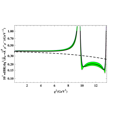
Figure 8: The differential width of $\bar{B}_{0}\to\bar{K}\mu^{+}\mu^{-}$, including the charm-loop effect calculated with the central values of input (solid, the shaded area indicates estimated uncertainties) and without this effect (dashed).

Table 2: Parameters of the ansatz (70) for $\Delta C_{9}^{(\bar{c}c,B\to K^{\ast},M_{i})}(q^{2})$ valid at $1.0<q^{2}<9.0$ GeV².

parameters	value at $\bar{q}^{2}=1.0$ GeV2	$r_{1}^{(B\to K^{*},{\cal M}_{i})}$	$r_{2}^{(B\to K^{*},{\cal M}_{i})}$
$\Delta C_{9}^{(\bar{c}c,B\to K^{\ast},M_{1})}$	$0.72^{+0.57}_{-0.37}$	$0.10^{+0.02}_{-0.00}$	$1.13^{+0.00}_{-0.01}$
$\Delta C_{9}^{(\bar{c}c,B\to K^{\ast},M_{2})}$	$0.76^{+0.70}_{-0.41}$	$0.09^{+0.01}_{-0.00}$	$1.12^{+0.00}_{-0.01}$
$\Delta C_{9}^{(\bar{c}c,B\to K^{\ast},M_{3})}$	$1.11^{+1.14}_{-0.70}$	$0.06^{+0.04}_{-0.10}$	$1.05^{+0.05}_{-0.04}$

For the phenomenologically interesting region $1.0<q^{2}<9.0$ GeV² we suggest the following numerical parameterizations of these corrections:

$$\Delta C_{9}^{(\bar{c}c,B\to K^{\ast},{\cal M}_{i})}(q^{2})=\frac{r_{1}^{(B\to K^{*},{\cal M}_{i})}\left(1-\frac{\bar{q}^{2}}{q^{2}}\right)+\Delta C_{9}^{(\bar{c}c,B\to K^{\ast},{\cal M}_{i})}(\bar{q}^{2})\frac{\bar{q}^{2}}{q^{2}}}{1+r_{2}^{(B\to K^{\ast},{\cal M}_{i})}\frac{\bar{q}^{2}-q^{2}}{m_{J/\psi}^{2}}}\,,$$ (70)

where the calculated values of $\Delta C_{9}^{(\bar{c}c,B\to K^{\ast},{\cal M}_{i})}(\bar{q}^{2}=1{\rm GeV^{2}})$ and the fitted values of $r_{1,2}^{(B\to K^{\ast},{\cal M}_{i})}$ are collected in Table 2.

In the region between $J/\psi$ and $\psi(2S)$ our results for $\Delta C_{9}^{\bar{c}c,B\to K^{(\ast)}}(q^{2})$ provide at most crude estimates. Nevertheless, this region is interesting because the predicted destructive interference between the $J/\psi$ and $\psi(2S)$ poles manifests itself in the form of a characteristic maximum located in the middle. In case of the constructive interference (which is demanding an unnaturally big, destructively interfering contribution of higher $\psi$-states in order to satisfy the dispersion relation) the maximum is replaced by a monotonously increasing curve.

At $q^{2}>m_{\psi(2S)}^{2}$, the dispersion relation becomes too complicated to be treated by any simple model, and the estimate of the charm-loop effect remains an open problem. From what we discussed above, it is obvious, that neither the approximation $\{$ $\bar{c}c$-loop $\oplus$ gluon corrections$\}$, nor a simple sum over $\psi$ resonances can provide an adequate description of this effect in $B\to K^{(*)}\ell^{+}\ell^{-}$.

We are now in a position to investigate the impact of the predicted charm-loop effect on the observables in $B\to K^{(\ast)}\ell^{+}\ell^{-}$. With the decay amplitudes defined in Appendix B the differential widths are calculated adding the charm-loop corrections to $C_{9}$. Since we are only interested in this effect, the other small nonfactorizable contributions (e.g.. the loops due to the quark-penguin operators or $u$-quark loops) are not taken into account. Remember that our analysis also does not include perturbative nonfactorizable effects, hence our calculated widths are strictly speaking not yet the complete predictions to be compared with the data. Furthermore, for the calculation of the $B\to K\ell^{+}\ell^{-}$ differential width we use the $B\to K$ vector and tensor form factors obtained from more accurate LCSR with kaon DA’s [18, 34] (see Appendix B). The result is plotted in Fig. 8. As expected, the charm-loop effect becomes essential only if one approaches the $J/\psi$ resonance region.

The same effect is significantly more pronounced in the differential width of $B\to K^{\ast}\ell^{+}\ell^{-}$, where in each $M_{i}$-part of the decay amplitude one has to replace $C_{9}$ by $C_{9}+\Delta C_{9}^{(\bar{c}c,B\to K^{*},{\cal M}_{i})}$. The result is presented in Fig. 9 where we normalize the width to its value at $q^{2}=1$ GeV² in order to diminish the large uncertainties contributing to the width by $B\to K^{*}$ form factors. The latter are calculated from LCSR with $B$ meson DA’s (see Appendix B).

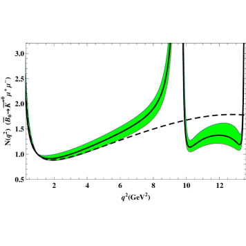
Figure 9: The differential width of $\bar{B}_{0}\to\bar{K}^{\ast}\mu^{+}\mu^{-}$ normalized at $q^{2}=1.0$ GeV², The notations are the same as in Fig. 8.

Finally, we consider the forward-backward asymmetry in $B\to K^{\ast}\ell^{+}\ell^{-}$ (for definition see e.g. [15] ). In our notations, the zero-point of this asymmetry is determined by the following equation

$$C_{7}^{eff}{m_{B}(m_{b}+m_{s})\over q_{0}^{2}}\bigg{[}\bigg{(}1+\frac{m_{K^{\ast}}}{m_{B}}\bigg{)}{T_{1}^{BK^{\ast}}(q_{0}^{2})\over V^{BK^{\ast}}(q_{0}^{2})}+\bigg{(}1-\frac{m_{K^{\ast}}}{m_{B}}\bigg{)}{T_{2}^{BK^{\ast}}(q_{0}^{2})\over A_{1}^{BK^{\ast}}(q_{0}^{2})}\bigg{]}$$

$$+C_{9}+\frac{1}{2}\bigg{[}\Delta C_{9}^{(\bar{c}c,B\to K^{*},{\cal M}_{1})}(q_{0}^{2})+\Delta C_{9}^{(\bar{c}c,B\to K^{*},{\cal M}_{2})}(q_{0}^{2})\bigg{]}=0\,.$$ (71)

The numerical result for the asymmetry is plotted in Fig. 10. Solving the above equation and taking into account the uncertainties we obtain

$$q^{2}_{0}=2.9^{+0.2}_{-0.3}{\rm GeV^{2}}\,$$ (72)

This is close to the prediction of [15] and the one (at the leading-order) of [4]. Since the above interval at least marginally belongs to the validity region of QCD calculation, the estimate (72) is practically independent of the dispersion-relation ansatz. Hence, we can clarify the influence of the nonfactorizable contribution on the position of the zero-point. Switching this contribution off, we observe a small shift of the central value towards $q^{2}_{0}=3.2~{}{\rm GeV^{2}}$. Note that, according to [4], the addition of perturbative NLO corrections, causes a significant shift of $q_{0}^{2}$ upwards.

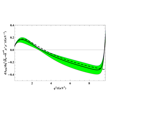
Figure 10: The forward-backward asymmetry for $\bar{B}_{0}\to\bar{K^{\ast}}\mu^{+}\mu^{-}$ decay. The notations are the same as in Figs 7,8.

8 Conclusion and outlook

In this paper we went beyond the perturbative approximation for the charm-loop effect in $B\to K^{(*)}\ell^{+}\ell^{-}$. In addition to the leading-order $c$-quark loop, the long-distance soft-gluon emission which violates factorization were taken into account. Employing the OPE near the light-cone, we derived a nonlocal effective operator responsible for the soft-gluon emission from the intermediate $c$-quarks. The $B\to K^{(*)}$ hadronic matrix element of this operator has a structure of nonforward (flavour changing) parton distribution, and has to be obtained from nonperturbative QCD. We employed LCSR with $B$- meson DA’s to calculate these matrix elements. The same method and input was used to obtain the $B\to K^{(*)}$ form factors entering the factorizable contribution. In the decay amplitudes, the new soft-gluon contribution becomes numerically important, being enhanced by its Wilson coefficient and by $\sim 1/q^{2}$ for $B\to K^{*}\ell^{+}\ell^{-}$ with respect to the factorizable part. The characteristic power suppression of the soft-gluon contribution is $\sim 1/(4m_{c}^{2}-q^{2})$, signaling that the approximation “perturbative loop $\oplus$ soft-gluon corrections” is only applicable at $q^{2}\ll 4m_{c}^{2}$. At $q^{2}$ approaching the ${\bar{c}}c$-threshold, multiple soft-gluon emission operators have to be included, new hadronic matrix elements proliferate and one eventually looses control over OPE. A clear footprints of these effects are the observed large violations of factorization in $B\to\mbox{charmonium}+K^{(*)}$ decays.

LCSR with $B$-meson DA’s used in this paper are not yet sufficiently accurate. There are unaccounted $\sim 1/m_{b}$ corrections to the HQET correlation function, the gluon radiative corrections are not taken into account and the parameters of $B$-meson DA’s, e.g., the inverse moment, still have large uncertainties. The imperfection of sum rules eventually converts into relatively large theoretical errors of our calculation. Nevertheless, since we are investigating a small effect, at least at low $q^{2}$, the achieved accuracy is reasonable. We believe that in future also other methods, first of all, lattice QCD can be used to calculate the $B\to K^{(*)}$ hadronic matrix elements emerging from the light-cone OPE. Also the conventional LCSR with light-mesons DA’s and $B$ -meson interpolating current can be employed for this purpose, with necessary modifications [24] (an artificial 4-momentum in the vertex of the effective operator).

In this paper we also applied the OPE-constrained dispersion relations for the $B\to K^{(*)}$ hadronic amplitudes with charm loop in order to to access the large $q^{2}$ region, including charmonium resonances. Our approach goes beyond the earlier ansatz [13, 15] in terms of dispersion relation, since we include nonfactorizable corrections and use the QCD result at small and spacelike $q^{2}$ to constrain the integral over higher states. This analysis clearly indicates a nontrivial interference between the contributions of $J/\psi$ and $\psi(2S)$ states.

One conclusion of our study sounds rather pessimistic. In our opinion, it is difficult, if not impossible at all to make a reliable prediction for the charm-loop effect above $\psi(2S)$, based on QCD. Although the actual effect could be small in this region, it will depend on the interference of many charmonium states and cannot be reliably constrained by OPE. In principle, new accurate data on the branching fractions $B\to\psi K^{(*)}$ for $\psi$ states heavier than $\psi(2S)$ and eventually also on $B\to\bar{D}DK^{(*)}$ can be used to saturate the spectral density of the charm loop amplitude at large $q^{2}$.

In this paper we considered only one, albeit important effect of four-quark operators with $c$ quarks in $B\to K^{(*)}\ell^{+}\ell^{-}$. Similar effects of quark loops with different flavours stemming from CKM suppressed and/or quark-penguin operators can be taken into account along the same lines. Note that in the case of light-quark loops, e.g., the $u$-quark loops important in $B\to\rho(\pi)\ell^{+}\ell^{-}$, one has to expand at large spacelike $q^{2}$. A separate interesting question deserving future study is the potential role of soft gluons in the weak annihilation contributions in rare semileptonic $B$ decays.

Appendix A: Effective Hamiltonian

For convenience, here we list all those operators $O_{i}$ and their Wilson coefficients $C_{i}$, entering $H_{eff}$ in (1) which are used throughout this paper omitting $O_{3-6}$ with very small Wilson coefficients and $O_{8g}$ :

$$O_{1} = \left(\bar{s}_{L}\gamma_{\rho}c_{L}\right)\left(\bar{c}_{L}\gamma^{\rho}b_{L}\right)\,,~{}~{}~{}O_{2}=\left(\bar{s}^{j}_{L}\gamma_{\rho}c^{i}_{L}\right)\left(\bar{c}^{i}_{L}\gamma^{\rho}b^{j}_{L}\right)\,,$$

$$O_{9} = \frac{\alpha_{em}}{4\pi}\left(\bar{s}_{L}\gamma_{\rho}b_{L}\right)\left(\bar{l}\gamma^{\rho}l\right)\,,~{}~{}~{}O_{10}=\frac{\alpha_{em}}{4\pi}\left(\bar{s}_{L}\gamma_{\rho}b_{L}\right)\left(\bar{l}\gamma^{\rho}\gamma_{5}l\right)\,,$$

$$O_{7\gamma} = -{e\over 16\pi^{2}}\bar{s}\sigma_{\mu\nu}(m_{s}L+m_{b}R)bF^{\mu\nu}\,,$$

where the notations $q_{L(R)}=\frac{1-(+)\gamma_{5}}{2}q$ and $L(R)=\frac{1-(+)\gamma_{5}}{2}$ are used. We use the standard conventions for the operators $O_{i}$, except the labelling of $O_{1}$ and $O_{2}$ is interchanged.

The sign convention for $O_{7\gamma}$ and $O_{8g}$ corresponds to the covariant derivative $iD_{\mu}=i\partial_{\mu}+eQ_{f}A_{\mu}+gT^{a}A^{a}_{\mu}$, where $Q_{f}$ is the fermion charge. In addition, the convention for the Levi-Civita tensor adopted in this work is ${\rm Tr}\{\gamma^{\mu}\gamma^{\nu}\gamma^{\rho}\gamma^{\lambda}\gamma^{5}\}=4i\epsilon^{\mu\nu\rho\lambda}\,,~{}\epsilon^{0123}=-1.$

We use the Wilson coefficients $C_{i}$ calculated in the leading approximation. They are given in Table 3.

Table 3: Numerical values of the Wilson coefficients at three different scales.

$\mu$ (GeV)	$0.5m_{b}$	$m_{b}$	$1.5m_{b}$
$C_{1}$	$1.180$	$1.117$	$1.090$
$C_{2}$	$-0.380$	$-0.267$	$-0.214$
$C_{7}^{eff}$	$-0.363$	$-0.319$	$-0.298$
$C_{9}$	$4.435$	$4.228$	$4.034$
$C_{10}$	$-4.410$	$-4.410$	$-4.410$

Appendix B: Decay amplitudes and form factors

1. $B\to K\ell^{+}\ell^{-}$

The dominant contributions to the amplitude $B\to K\ell^{+}\ell^{-}$ stem from the hadronic matrix elements of the operators $O_{7\gamma}$, $O_{9}$ and $O_{10}$:

$$A(B\to K\ell^{+}\ell^{-}) = {G_{F}\over\sqrt{2}}{\alpha_{em}\over\pi}V_{tb}V_{ts}^{\ast}\Bigg{[}\bar{\ell}\gamma_{\mu}\ell\,p^{\mu}\bigg{(}C_{9}f^{+}_{BK}(q^{2})$$ (73)

$$+{2(m_{b}+m_{s})\over m_{B}+m_{K}}C_{7}^{eff}f^{T}_{BK}(q^{2})\bigg{)}+\bar{\ell}\gamma_{\mu}\gamma_{5}\ell\,p^{\mu}C_{10}f^{+}_{BK}(q^{2})\bigg{]}\,,\hskip 76.82234pt$$

where we omit the contributions yielding the lepton mass (the latter are included in the numerical analysis). The tensor $B\to K$ form factor is defined as

$$\langle K(p)|\bar{s}\sigma_{\mu\rho}q^{\rho}b|B(p+q)\rangle=\bigg{[}q^{2}(2p_{\mu}+q_{\mu})-(m_{B}^{2}-m_{K}^{2})q_{\mu}\bigg{]}\frac{if^{T}_{BK}(q^{2})}{m_{B}+m_{K}}\,.$$ (74)

2. $B\to K^{*}\ell^{+}\ell^{-}$

For $B\to K^{*}\ell^{+}\ell^{-}$ decay amplitude we use the following expression:

$$A(B\to K^{\ast}l^{+}l^{-}) = {G_{F}\over 2\sqrt{2}}{\alpha_{em}\over\pi}V_{tb}V_{ts}^{\ast}\Bigg{\{}\bar{l}\gamma^{\mu}l\Big{[}\epsilon_{\mu\nu\rho\sigma}\epsilon^{\ast\nu}q^{\rho}p^{\sigma}{\cal M}_{1}(q^{2})$$

$$-i\epsilon^{\ast}_{\mu}{\cal M}_{2}(q^{2})+i(\epsilon^{\ast}\cdot q)p_{\mu}{\cal M}_{3}(q^{2})\Big{]}$$

$$+\bar{l}\gamma^{\mu}\gamma_{5}l\Big{[}\epsilon_{\mu\nu\rho\sigma}\epsilon^{\ast\nu}q^{\rho}p^{\sigma}{\cal N}_{1}(q^{2})-i\epsilon^{\ast}_{\mu}{\cal N}_{2}(q^{2})+i(\epsilon^{\ast}\cdot q)p_{\mu}{\cal N}_{3}(q^{2})\Big{]}\Bigg{\}}\,,\hskip 28.45274pt$$

where

$${\cal M}_{1}(q^{2}) = C_{9}{2V^{BK^{\ast}}(q^{2})\over m_{B}+m_{K^{\ast}}}+4C_{7}^{eff}{m_{b}+m_{s}\over q^{2}}T_{1}^{BK^{\ast}}(q^{2})\,,$$

$${\cal M}_{2}(q^{2}) = C_{9}(m_{B}+m_{K^{\ast}})A_{1}^{BK^{\ast}}(q^{2})$$

$$+2C_{7}^{eff}(m_{B}^{2}-m_{K^{\ast}}^{2}){m_{b}+m_{s}\over q^{2}}T_{2}^{BK^{\ast}}(q^{2})\,,$$

$${\cal M}_{3}(q^{2}) = 2C_{9}{A_{2}^{BK^{\ast}}(q^{2})\over m_{B}+m_{K^{\ast}}}$$ (76)

$$+4C_{7}^{eff}{m_{b}-m_{s}\over q^{2}}\bigg{(}T_{2}^{BK^{\ast}}(q^{2})+{q^{2}\over m_{B}^{2}-m_{K^{\ast}}^{2}}T_{3}^{BK^{\ast}}(q^{2})\bigg{)}\,,\,\,\,\,\,\,\,$$

and

$${\cal N}_{1}(q^{2}) = 2C_{10}{V^{BK^{\ast}}(q^{2})\over m_{B}+m_{K^{\ast}}},\qquad{\cal N}_{2}(q^{2})=C_{10}({m_{B}+m_{K^{\ast}}})A_{1}^{BK^{\ast}}(q^{2})\,,$$

$${\cal N}_{3}(q^{2}) = 2C_{10}{A_{2}^{BK^{\ast}}(q^{2})\over m_{B}+m_{K^{\ast}}}\,.$$ (77)

The tensor $B\to K^{\ast}$ form factors are defined as

$$\langle K^{\ast}(p)|\bar{s}\sigma_{\mu\rho}q^{\rho}(1+\gamma_{5})b|B(p+q)\rangle=2i\epsilon_{\mu\nu\rho\sigma}\epsilon^{\ast\nu}q^{\rho}p^{\sigma}T_{1}^{BK^{\ast}}(q^{2})$$

$$+[(m_{B}^{2}-m^{2}_{K^{\ast}}){\epsilon}^{\ast}_{\mu}-(\epsilon^{\ast}\!\cdot q)(2p+q)_{\mu}]T_{2}^{BK^{\ast}}(q^{2})$$

$$+(\epsilon^{\ast}\!\cdot q)\bigg{[}q_{\mu}-{q^{2}\over m_{B}^{2}-m^{2}_{K^{\ast}}}(2p+q)_{\mu}\bigg{]}T_{3}^{BK^{\ast}}(q^{2})\,,$$ (78)

with $T_{1}^{BK^{\ast}}(0)=T_{2}^{BK^{\ast}}(0)$.

3. $B\to K^{*}\gamma$

The amplitude of $B\to K^{\ast}\gamma$ decay is

$$A(B\to K^{\ast}\gamma)={G_{F}\over\sqrt{2}}{e\over 2\pi^{2}}V_{tb}V_{ts}^{*}C_{7}^{eff}\Big{\{}-(m_{b}+m_{s})\epsilon_{\mu\nu\rho\sigma}\epsilon^{\ast\mu}_{\gamma}\epsilon^{\ast\nu}q^{\rho}p^{\sigma}$$

$$+i(m_{b}-m_{s})\big{[}(\epsilon^{\ast}\cdot\epsilon^{\ast}_{\gamma})(p\cdot q)-(\epsilon^{\ast}\cdot q)(\epsilon^{\ast}_{\gamma}\cdot p)\big{]}\Big{\}}T_{1}^{BK^{\ast}}(0)\,,$$ (79)

where $\epsilon^{\ast}_{\gamma}$ is the polarization vector of the photon.

4. $B\to K^{(*)}$ form factors

The $B\to K^{(\ast)}$ form factors used in the factorizable parts of the charm-loop effect calculation are substituted by the corresponding LCSR with $B$ meson DA’s. For the differential widths we need an explicit numerical parameterization of these and also tensor form factors. We parameterize the $q^{2}$-dependence of all $B\to K^{(\ast)}$ form factors with the $z$-parameterization similar to the one suggested in [35], with one slope parameter:

$$F(q^{2})=\frac{F(0)}{1-q^{2}/m^{2}_{B_{s}(J^{P})}}\bigg{\{}1+b_{1}\bigg{(}z(q^{2},t_{0})-z(0,t_{0})+\frac{1}{2}\big{[}z(q^{2},t_{0})^{2}-z(0,t_{0})^{2}\big{]}\bigg{)}\bigg{\}}\,,$$ (80)

and

$$z(q^{2},\tau_{0})={\sqrt{\tau_{+}-q^{2}}-\sqrt{\tau_{+}-\tau_{0}}\over\sqrt{\tau_{+}-q^{2}}+\sqrt{\tau_{+}-\tau_{0}}}\,,$$

$$\tau_{+}=(m_{B}+m_{K^{(\ast)}})^{2}\,,\qquad\tau_{-}=(m_{B}-m_{K^{(\ast)}})^{2}$$

$$\tau_{0}=\tau_{+}-\sqrt{\tau_{+}-\tau_{-}}\sqrt{\tau_{+}}\,.$$ (81)

The pole corresponds to the $\bar{s}b$- resonance with appropriate $J^{P}$. The $B\to K$ form factors are calculated from more accurate LCSR with kaon DA’s [18, 34] at $q^{2}<12$ GeV² including the spacelike region, and the result is fitted to the above parameterization. The $B\to K^{*}$ form factors are calculated from LCSR with $B$ meson DA’s [11] in the same region. For the two tensor form factors $T_{2,3}$ the results are new. The form factor values at $q^{2}=0$ and the fitted slope parameters are presented in Table 4, where the masses of the $B_{s}$ states are [36]: $m_{B_{s}(0^{-})}=5.366$ GeV, $m_{B_{s}^{*}(1^{-})}=5.412$ GeV and  $m_{B_{s}^{*}(1^{+})}=5.829$ GeV. Within uncertainties, the form factors obtaned from the two different LCSR agree with each other (see[11]).

form factor	$F^{i}_{BK^{(\ast)}}(0)$	$b_{1}^{i}$	$B_{s}(J^{P})$	input
				at $q^{2}<12$ GeV2
$f_{BK}^{+}$	$0.34^{+0.05}_{-0.02}$	$-2.1^{+0.9}_{-1.6}$	$B_{s}^{*}(1^{-})$
$f_{BK}^{0}$	$0.34^{+0.05}_{-0.02}$	$-4.3^{+0.8}_{-0.9}$	no pole	LCSR
$f_{BK}^{T}$	$0.39^{+0.05}_{-0.03}$	$-2.2^{+1.0}_{-2.00}$	$B_{s}^{*}(1^{-})$	with $K$ DA’s
$V^{BK^{\ast}}$	$0.36^{+0.23}_{-0.12}$	$-4.8^{+0.8}_{-0.4}$	$B_{s}^{*}(1^{-})$
$A_{1}^{BK^{\ast}}$	$0.25^{+0.16}_{-0.10}$	$0.34^{+0.86}_{-0.80}$	$B_{s}(1^{+})$
$A_{2}^{BK^{\ast}}$	$0.23^{+0.19}_{-0.10}$	$-0.85^{+2.88}_{-1.35}$	$B_{s}(1^{+})$	LCSR
$A_{0}^{BK^{\ast}}$	$0.29^{+0.10}_{-0.07}$	$-18.2^{+1.3}_{-3.0}$	$B_{s}(0^{-})$	with $B$ DA’s
$T_{1}^{BK^{\ast}}$	$0.31^{+0.18}_{-0.10}$	$-4.6^{+0.81}_{-0.41}$	$B_{s}^{*}(1^{-})$
$T_{2}^{BK^{\ast}}$	$0.31^{+0.18}_{-0.10}$	$-3.2^{+2.1}_{-2.2}$	$B_{s}(1^{+})$
$T_{3}^{BK^{\ast}}$	$0.22^{+0.17}_{-0.10}$	$-10.3^{+2.5}_{-3.1}$	$B_{s}(1^{+})$

Table 4: The $B\to K^{(\ast)}$ form factors from LCSR and their $z$-parameterization.

Appendix C: Parameters of $\psi=\{J/\psi,\psi(2S)\}$ and $B\to\psi K^{(*)}$ amplitudes

The necessary data on the two lowest charmonium levels are collected in Table 5, where also the absolute values of the $B\to\psi K$ decay amplitudes are given, calculated from:

$$|A_{B\psi K}|=\Bigg{(}\frac{8\pi BR(B\to\psi K)}{\tau(B)G_{F}^{2}|V_{cs}|^{2}|V_{cb}|^{2}m_{B}^{3}\lambda^{3/2}_{B\psi K}}\Bigg{)}^{1/2}\,,$$ (82)

where $\lambda_{B\psi K}=\lambda(1,m_{K}^{2}/m_{B}^{2},m_{\psi}^{2}/m_{B}^{2})$, and $\lambda(a,b,c)\equiv a^{2}+b^{2}+c^{2}-2ab-2ac-2bc$.

For $B\to\psi K^{*}$ we use the decomposition in transversity amplitudes:

$$\langle K^{\ast}(p)\psi(q)|\left(C_{1}O_{1}+C_{2}O_{2}\right)|B(p+q)\rangle$$

$$=i\sqrt{2}{\epsilon}_{\alpha}{\epsilon_{\psi}}_{\beta}\Bigg{\{}i\epsilon^{\alpha\beta\rho\tau}p_{\rho}q_{\tau}\frac{A^{\perp}_{B\psi K^{*}}}{m_{B}^{2}\lambda_{B\psi K^{*}}^{1/2}}+g^{\alpha\beta}\frac{A^{\parallel}_{B\psi K^{*}}}{2}$$ (83)

$$+\frac{1}{m_{B}^{4}\lambda_{B\psi K^{*}}}(p+q)^{\alpha}(p+q)^{\beta}\Big{[}2m_{K^{\ast}}m_{\psi}A^{0}_{B\psi K^{*}}-(m_{B}^{2}-m_{\psi}^{2}-m_{K^{\ast}}^{2})A^{\parallel}_{B\psi K^{*}}\Big{]}\Bigg{\}}\,,\hskip 28.45274pt$$

where $\lambda_{B\psi K^{*}}=\lambda(1,{m^{2}_{K^{\ast}}/m_{B}^{2}},{m_{\psi}^{2}/m_{B}^{2}})$, so that the decay width is

$$\Gamma(B\to\psi K^{\ast})=\frac{\lambda_{B\psi K^{*}}^{1/2}}{16\pi m_{B}}\bigg{(}{4G_{F}\over\sqrt{2}}\bigg{)}^{2}|V_{cb}V^{\ast}_{cs}|^{2}\sum_{i=0,\parallel,\perp}|A^{i}_{B\psi K^{*}}|^{2}\,.$$ (84)

The polarization fractions $f_{i}(i=0,\parallel,\perp)$ are defined as follows:

$$f_{i}=\frac{|A_{B\psi K^{*}}^{i}|^{2}}{|A_{B\psi K^{*}}^{0}|^{2}+|A_{B\psi K^{*}}^{\parallel}|^{2}+|A_{B\psi K^{*}}^{\perp}|^{2}}\;.$$ (85)

The transversity amplitudes in this decay can be determined from the data on the branching fractions and polarization fractions collected in Table 5. In addition, one can determine the relative sign between $A_{0}$ and $A_{\parallel}$.

state	$J/\psi$	$\psi(2S)$
Mass (${\rm MeV}$)	$3096.916\pm 0.011$	$3686.09\pm 0.04$
$\Gamma_{tot}\,\,({\rm keV})$	$93.2\pm 2.1$	$317\pm 9$
$\Gamma_{ll}\,\,({\rm keV})$	$5.55\pm 0.14\pm 0.02$	$2.38\pm 0.04$
$f_{\psi}\,\,({\rm MeV})$	$416^{+5}_{-6}$	$297^{+3}_{-2}$
$BR(\bar{B}^{0}\to J/\psi K^{0})$	$8.63\pm 0.35\times 10^{-4}$	$6.55\pm 0.66\times 10^{-4}$
$|A_{B\psi K}|(\rm MeV)$	$31^{+3}_{-1}$	$41^{+4}_{-2}$
$BR(\bar{B}^{0}\to J/\psi K^{\ast 0})$	$13.3\pm 0.7\times 10^{-4}$	$7.10\pm 0.62\times 10^{-4}$
$f_{0}$	$0.556\pm 0.009\pm 0.010$	$0.48\pm 0.05\pm 0.02$
$f_{\|}$	$0.211\pm 0.010\pm 0.006$	$0.22\pm 0.06\pm 0.02$
$f_{\perp}$	$0.233\pm 0.010\pm 0.005$	$0.30\pm 0.06\pm 0.02$
$|A_{0}|(\rm GeV^{3})$	$0.27^{+0.00}_{-0.01}$	$0.22^{+0.01}_{-0.02}$
$|A_{\|}|(\rm GeV^{3})$	$0.16^{+0.01}_{-0.00}$	$0.15^{+0.02}_{-0.03}$
$|A_{\perp}|(\rm GeV^{3})$	$0.17^{+0.01}_{-0.00}$	$0.17^{+0.02}_{-0.02}$

Table 5: The characteristics of $J/\psi$ and $\psi(2S)$ taken from [31, 33].

Appendix D: The coefficients in the LCSR

The resulting expressions for the coefficients $C^{(F)}(q^{2},u,\sigma,\omega,t)$ entering the sum rule (4), $F=\Psi_{V},\Psi_{AV},...$ are presented here in a form of the quadratic polynomials in the variable $\omega$,

$$C^{(F)}(q^{2},u,\sigma,\omega,t)=\sum\limits_{r=0,1,2}C^{(F)}_{r}(q^{2},u,\sigma,t)~{}\left(\frac{\omega}{m_{B}}\right)^{r}\,.$$

The nonvanishing coefficients of these polynomials are:

$$C^{(\Psi_{V})}_{0} = (1-t)t\left[2\text{q2}((2\text{sig}-5)u+2)-2\text{mB}^{2}(\text{sig}-1)^{2}(u-1)\right]$$

$$-\frac{1}{2}\text{q2}(2\text{sig}-3)(2u-1)\,,$$

$$C^{(\Psi_{V})}_{1} = 4(1-t)tu\left[\text{mB}^{2}(\text{sig}(2(\text{sig}-4)u-\text{sig}+5)+7u-4)+2\text{q2}(u-1)\right]$$

$$+\text{mB}^{2}(2\text{sig}-3)u(2u-1)\,,$$

$$C^{(\Psi_{V})}_{2} = 8\text{mB}^{2}(1-t)tu^{2}(\text{sig}(4u-3)-3u+3)\,;$$ (86)

$$C^{(\Psi_{AV})}_{0} = (1-t)t\big{[}\text{mB}^{2}(\text{sig}-1)^{2}(u-2)-\text{q2}(6\text{sig}u+u-2)\big{]}+\text{q2}\text{sig}(2u-1)\,,$$

$$C^{(\Psi_{AV})}_{1} = -\frac{2(1-t)tu}{\text{sig}-1}\bigg{(}\text{mB}^{2}(\text{sig}-1)\big{[}\text{sig}(2\text{sig}(u-1)-7u+4)+u-2\big{]}$$ (87)

$$+\text{q2}(2\text{sig}+u-2)\bigg{)}+2\text{mB}^{2}\text{sig}(1-2u)u\,;$$

$$C^{(XA)}_{0} = \frac{(1-t)t\left[\text{mB}^{2}(\text{sig}-1)^{2}(u-2)+\text{q2}((5-6\text{sig})u-2)\right]}{\text{mB}(\text{sig}-1)}$$

$$+\frac{\text{q2}(2\text{sig}-1)(2u-1)}{2\text{mB}(\text{sig}-1)}\,,$$

$$C^{(X_{A})}_{1} = \frac{4(1-t)tu\left[\text{mB}^{2}\left((\text{sig}-1)^{2}-((\text{sig}-4)\text{sig}+2)u\right)+\text{q2}(1-u)\right]}{\text{mB}(\text{sig}-1)}$$ (88)

$$+\frac{\text{mB}u(2u-1)(1-2\sigma)}{\text{sig}-1}\,;$$

$$\widetilde{C}^{(X_{A})}_{0} = \frac{2\text{q2}(1-t)tu\big{[}\text{mB}^{2}(\text{sig}-1)^{2}+\text{q2}(2\text{sig}-1)\big{]}}{\text{mB}^{3}(\text{sig}-1)}$$

$$-\frac{\text{q2}(2u-1)\left[\text{mB}^{2}(\text{sig}-1)^{2}+\text{q2}(2\text{sig}-1)\right]}{2\text{mB}^{3}(\text{sig}-1)}\,,$$

$$\widetilde{C}^{(X_{A})}_{1} = \frac{u(2u-1)\left[\text{mB}^{2}(\text{sig}-1)^{2}+\text{q2}(2\text{sig}-1)\right]}{\text{mB}(\text{sig}-1)}$$ (89)

$$-\frac{4(1-t)tu^{2}\left[\text{mB}^{2}(\text{sig}-1)^{2}+\text{q2}(2\text{sig}-1)\right]}{\text{mB}(\text{sig}-1)}\,;$$

$$C^{(Y_{A})}_{0} = -2\text{mB}(\text{sig}-1)(1-t)t(u-2)\,,~{}~{}~{}$$

$$C^{(Y_{A})}_{1} = 8\text{mB}(\text{sig}+1)(1-t)t(u-1)u\,,$$

$$C^{(Y_{A})}_{2} = 8\text{mB}(1-t)tu^{2}\left(\frac{(3-2\text{sig})u}{\text{sig}-1}+4\right)\,;$$ (90)

$$\widetilde{C}^{(Y_{A})}_{0} = \frac{2}{\text{mB}}(\text{sig}-1)(1-t)t\big{(}\text{mB}^{2}(\text{sig}-1)^{2}(u-2)$$

$$-\text{q2}(6\text{sig}u+u-2)\big{)}+\frac{2\text{q2}(\text{sig}-1)\text{sig}(2u-1)}{\text{mB}}\,,$$

$$\widetilde{C}^{(Y_{A})}_{1} = -\frac{8}{\text{mB}}(1-t)tu\big{[}\text{mB}^{2}(\text{sig}-1)(\text{sig}(\text{sig}(u-1)-4u+3)+u-2)$$

$$+\text{q2}(\text{sig}u+\text{sig}+u-2)\big{]}-4\text{mB}(\text{sig}-1)\text{sig}\,,$$

$$\widetilde{C}^{(Y_{A})}_{2} = -\frac{8}{\text{mB}(\text{sig}-1)}(1-t)tu^{2}\big{[}\text{mB}^{2}(\text{sig}-1)^{2}(2\text{sig}(u-1)-u+2)$$ (91)

$$+\text{q2}(2\text{sig}+u-2)\big{]}\,.$$

References

• [1] B. Grinstein, M.J. Savage and M.B. Wise, Nucl. Phys. B319 (1989) 271; M. Misiak, Nucl. Phys. B393 (1993) 23; A.J. Buras and M. Munz, Phys. Rev. D52 (1995) 186.
• [2] G. Buchalla, A. J. Buras and M. E. Lautenbacher, Rev. Mod. Phys.  68 (1996) 1125.
• [3] CKMfitter Group (J. Charles et al.), Eur. Phys. J. C41, 1-131 (2005), http://ckmfitter.in2p3.fr .
• [4] M. Beneke, T. Feldmann and D. Seidel, Nucl. Phys.  B 612 (2001) 25.
• [5] M.B. Voloshin, Phys. Lett. B397 (1997) 275.
• [6] A. Khodjamirian, R. Ruckl, G. Stoll and D. Wyler, Phys. Lett. B402 (1997) 167.
• [7] P. Ball, G. W. Jones and R. Zwicky, Phys. Rev.  D 75 (2007) 054004.
• [8] Z. Ligeti, L. Randall and M.B. Wise, Phys. Lett. B402 (1997) 178: A.K. Grant, A.G. Morgan, S. Nussinov and R.D. Peccei, Phys. Rev. D56 (1997) 3151; J. W. Chen, G. Rupak and M. J. Savage, Phys. Lett.  B 410 (1997) 285.
• [9] G. Buchalla, G. Isidori and S.J. Rey, Nucl. Phys. B511 (1998) 594.
• [10] A. Khodjamirian, T. Mannel and N. Offen, Phys. Lett.  B 620 (2005) 52.
• [11] A. Khodjamirian, T. Mannel and N. Offen, Phys. Rev.  D 75 (2007) 054013.
• [12] A. Ali, T. Mannel and T. Morozumi, Phys. Lett. B273 (1991) 505.
• [13] F. Krüger and L.M. Sehgal, Phys. Lett. B380 (1996) 199.
• [14] M. Beneke, G. Buchalla, M. Neubert and C. T. Sachrajda, Eur. Phys. J.  C 61 (2009) 439.
• [15] A. Ali, P. Ball, L. T. Handoko and G. Hiller, Phys. Rev.  D 61 (2000) 074024.
• [16] P. Colangelo and A. Khodjamirian, arXiv:hep-ph/0010175.
• [17] P. Ball and R. Zwicky, Phys. Rev.  D 71, 014015 (2005); Phys. Rev.  D 71, 014029 (2005).
• [18] G. Duplancic, A. Khodjamirian, T. Mannel, B. Melic and N. Offen, JHEP 0804 (2008) 014.
• [19] S. W. Bosch and G. Buchalla, Nucl. Phys.  B 621 (2002) 459, A. Ali and A. Y. Parkhomenko, Eur. Phys. J.  C 23 (2002) 89, A. Ali, G. Kramer and G. h. Zhu, Eur. Phys. J.  C 47 (2006) 625.
• [20] I. I. Balitsky and V. M. Braun, Nucl. Phys.  B 311 (1989) 541.
• [21] V.M. Belyaev, V.M. Braun, A. Khodjamirian and R. Ruckl, Phys. Rev. D51 (1995) 6177.
• [22] A. Khodjamirian and R. Ruckl, in Heavy Flavors, 2nd edition, eds., A.J. Buras and M. Linder, Adv. Ser. Direct. High Energy Phys.  15, 345 (1998) (World Scientific) [arXiv:hep-ph/9801443].
• [23] S. J. Lee, M. Neubert and G. Paz, Phys. Rev.  D 75 (2007) 114005, M. Benzke, S. J. Lee, M. Neubert and G. Paz, arXiv:1003.5012 [hep-ph].
• [24] A. Khodjamirian, Nucl. Phys.  B 605 (2001) 558
• [25] B. Melic, Phys. Rev.  D 68 (2003) 034004.
• [26] H. Kawamura, J. Kodaira, C. F. Qiao and K. Tanaka, Phys. Lett. B 523, 111 (2001) [Erratum-ibid. B 536, 344 (2002)].
• [27] V. M. Braun, D. Y. Ivanov and G. P. Korchemsky, Phys. Rev.  D 69 (2004) 034014.
• [28] K. G. Chetyrkin, J. H. Kühn, A. Maier, P. Maierhofer, P. Marquard, M. Steinhauser and C. Sturm, Phys. Rev.  D 80 (2009) 074010.
• [29] K. G. Chetyrkin and A. Khodjamirian, Eur. Phys. J.  C 46 (2006) 721;
M. Jamin, J. A. Oller and A. Pich, Phys. Rev.  D 74 (2006) 074009.
• [30] M. Beneke, G. Buchalla, M. Neubert and C. T. Sachrajda, Phys. Rev. Lett.  83 (1999) 1914; Nucl. Phys.  B 606 (2001) 245.
• [31] Heavy Flavor Averaging Group, www.slac.stantford.edu/xorg/hfag/.
• [32] M. Beneke, J. Rohrer and D. Yang, Nucl. Phys.  B 774, 64 (2007).
• [33] B. Aubert et al. [BABAR Collaboration], Phys. Rev.  D 76 (2007) 031102.
• [34] G. Duplancic and B. Melic, Phys. Rev.  D 78 (2008) 054015.
• [35] C. Bourrely, I. Caprini and L. Lellouch, Phys. Rev.  D 79 (2009) 013008.
• [36] C. Amsler et al. [Particle Data Group], Phys. Lett.  B 667 (2008) 1.