Suppression of thermal conductivity in graphene nanoribbons with rough edges

Abstract

We analyze numerically the thermal conductivity of carbon nanoribbons with ideal and rough edges. We demonstrate that edge disorder can lead to a suppression of thermal conductivity by several orders of magnitude. This effect is associated with the edge-induced Anderson localization and suppression of the phonon transport, and it becomes more pronounced for longer nanoribbons and low temperatures.

I Introduction

The study of remarkable properties of graphite structures is one of the hot topics of nanoscience Katsnelson (2007). Graphene nanoribbons (GNRs) are effectively low-dimensional structures similar to carbon nanotubes, but their main feature is the presence of edges. Due to the edges, graphene nanoribbons can demonstrate many novel properties driven by their geometry, depending on their width and helicity. A majority of the current studies of graphene nanoribbons are devoted to the analysis of their electronic and magnetic properties modified by the presence of edges, including the existence of the localized edge modes Lee and Cho (2009); Engelund et al. (2010), which are an analog of surface states in the two-dimensional geometry. The edge can support localized vibrational states in both linear and nonlinear regimes Savin and Kivshar (2010a, b).

The effect of the edge disorder on the electronic transport of graphene nanoribbons has been discussed in several papers (see, e.g., Refs.  Evaldsson et al. (2008); Cresti and Roche (2009); Martin and Blanter (2009)). It was found that already very modest edge disorder is sufficient to induce the conduction energy gap in the otherwise metallic nanoribbons and to lift any difference in the conductance between nanoribbons of different edge geometry, suggesting that this type of disorder can be very important for altering other fundamental characteristics of GHRs.

In addition to electronic properties, the thermal properties of graphene are also of both fundamental and practical importance. Several experiments Ghosh et al. (2008); Balandin et al. (2008) have demonstrated that graphene has a superior thermal conductivity, likely underlying the high thermal conductivity known in carbon nanotubes Pop et al. (2006). This opens numerous possibilities for using graphene nanostructures in nanoscale thermal circuit management.

Recent experiments demonstrated that thermal conductivity of silicon nanowires can be dramatically reduced by surface roughness Hochbaum et al. (2008); Boukai et al. (2008). This results has been confirmed theoretically in the framework of a simplest phenomenological model of quasi-one-dimensional crystal that demonstrates the reduction of thermal conductivity due to roughness-induced disorder Kosevich and Savin (2009). Molecular dynamics simulations Hu et al. (2009) demonstrated that thermal conductivity of GRNs depends on the edge chirality and can be affected by defects. Therefore, we wonder if the edge disorder of GNRs can modify substantially their thermal conductivity, similar to the case of silicon nanowires.

In this Article, we study the thermal conductivity of isolated graphene nanoribbons with ideal and rough edges. By employing a direct modeling of heat transfer by means of the molecular-dynamics simulations, we demonstrate that the thermal conductivity grows monotonically with the GNR length as a power-law function. In contrast, rough edges of the nanoribbon can reduce the thermal conductivity by several orders of magnitude. This effect is enhanced for longer GNRs and for lower temperatures, and it corresponds to dramatic suppression of phonon transport solely by the edge disorder. It means that nanoribbons with ideal edges can play a role of highly efficient conductors in nanocircuits, whereas the rough edges will transform them into efficient thermal resistors.

II Model

We model a graphene nanoribbon as a planar strip of graphite, with the properties depending on the stripe width and chirality. The structure of the zigzag nanoribbon can be presented as a longitudinal repetition of the elementary cell composed $K$ atoms (the even number $K\geq 4$). We use atom numbering shown in Fig. 1(a). In this case, each carbon atoms has a two-component index $\alpha=(n,k)$, where $n=0,\pm 1,\pm 2,...$ stands for the number of the elementary cells, and $k=1,2,...,K$ stands for the number atoms in the cell.

Each elementary cell of the zigzag nanoribbon has two edge atoms. In Fig. 1(a), we show these edge atoms as filled circles. We consider a hydrogen-terminated nanoribbon, where edge atoms correspond to the molecular group CH. We consider such a group as a single effective particle at the location of the carbon atom. Therefore, in our model of graphene nanoribbon we take the mass of atoms inside the strip as $M_{0}=12m_{p}$, and for the edge atoms we consider a large mass $M_{1}=13m_{p}$ (where $m_{p}=1.6603\cdot 10^{-27}$kg is the proton mass).

Figure 1: (a) Schematic view of a zigzag nanoribbon with rough edges and atom numbering. The edge atoms are shown as filled circles. Dotted lines separate the elementary cells of the nanoribbon. $K$ is the number of atoms in the elementary cell. (b) Configurations of an ideal structure containing up to $i$-th nearest-neighbor interactions for $i=1,...,5$.

To model two rough edges we randomly delete some atoms with second index $k=1$ and $k=K$. Let $0\leq p\leq 1$ be the probability of atom removal. As a result of the random atom removal from the edge layers, some atoms at the edges will have only one covalent bond C–C and should be deleted as well. After this operation, the edge become rough, as shown in Fig. 2. Here all edge atoms participate only in two valent bonds C–C. We characterize the degree of roughness by the parameter $d=N_{a}/N_{b}$, where $N_{a}$ is the number of atoms in an ideal nanoribbon, and $N_{b}$ is the number of atoms remaining in the edge-disordered nanoribbon after removing some of the edge atoms. Parameter $d$ characterizes the density of the edge-disordered nanoribbon in comparison with the ideal case. When the probability $p$ for removal of an edge atom is $p=0$, we have $d=1$, and $d$ decays for larger values of the density $p$, so that for $p=1$ (when all atoms with the second index $k=1,2$ and $k=K-1,K$ are removed), it takes the minimum value $d=(K-4)/K$ (for $p=1$ we have again an ideal ribbon but for a smaller width, with $K-4$ atoms in an elementary cell). For $K=12$ and probability $p=0.5$ the density is $d=0.87$: this nanoribbon is shown in Fig. 2.

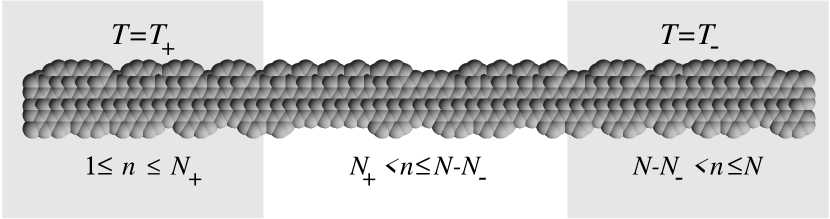
Figure 2: Example of a zigzag nanoribbon with rough edges with $N$ longitudinal segments. First left $N_{+}$ segments are attached to the $T=T_{+}$ thermostat and the last right $N_{-}$ segments are attached to the $T=T_{-}$ thermostat. Number of atoms in the elementary cell $K=12$, density of the nanoribbon with rough edges $d=0.87$ (probability $p=0.5$).

To describe the dynamics of both ideal and disordered nanoribbons, we present the system Hamiltonian in the form,

$$H=\sum_{n=-\infty}^{+\infty}\sum_{k=1}^{K_{n}}\left[\frac{1}{2}M_{(n,k)}(\dot{\bf u}_{(n,k)},\dot{\bf u}_{(n,k)})+P_{(n,k)}\right],$$ (1)

where $K-4\leq K_{n}\leq K$ is the number of atoms in the $n$-th elementary cell, $M_{\alpha}$ is the mass of the hydrogen atom with the index $\alpha=(n,k)$ (for internal atoms we take $M_{\alpha}=M_{0}$, whereas for the edge atoms we take a larger mass, $M_{\alpha}=M_{1}>M_{0}$), ${\bf u}_{\alpha}=(x_{\alpha}(t),y_{\alpha}(t),z_{\alpha}(t))$ is the radius-vector of the carbon atom with the index $\alpha$ at the moment $t$. The term $P_{\alpha}$ describes the interaction of the atom with the index $\alpha=(n,k)$ with its neighboring atoms. The potential depends on variations of bond length, bond angles, and dihedral angles between the planes formed by three neighboring carbon atoms, and it can be written in the form

$$P=\sum_{\Omega_{1}}U_{1}+\sum_{\Omega_{2}}U_{2}+\sum_{\Omega_{3}}U_{3}+\sum_{\Omega_{4}}U_{4}+\sum_{\Omega_{5}}U_{5},$$ (2)

where $\Omega_{i}$, with $i=1,2,3,4,5$ stand for the sets of configurations including up to nearest-neighbor interactions. Owing to a large redundancy, the sets only need to contain configurations of the atoms shown in Fig. 1(b), including their rotated and mirrored versions.

The potential $U_{1}({\bf u}_{\alpha},{\bf u}_{\beta})$ describes the deformation energy due to a direct interaction between pairs of atoms with the indices $\alpha$ and $\beta$, as shown in Fig. 1(b). The potential $U_{2}({\bf u}_{\alpha},{\bf u}_{\beta},{\bf u}_{\gamma})$ describes the deformation energy of the angle between the valent bonds ${\bf u}_{\alpha}{\bf u}_{\beta}$ and ${\bf u}_{\beta}{\bf u}_{\gamma}$. Potentials $U_{i}({\bf u}_{\alpha},{\bf u}_{\beta},{\bf u}_{\gamma},{\bf u}_{\delta})$, $i=3$, 4, 5, describes the deformation energy associated with a change of the effective angle between the planes ${\bf u}_{\alpha},{\bf u}_{\beta},{\bf u}_{\gamma}$ and ${\bf u}_{\beta},{\bf u}_{\gamma},{\bf u}_{\delta}$.

We use the potentials employed in the modeling of the dynamics of large polymer macromolecules Noid et al. (1991); Savin and Manevitch (2003) for the valent bond coupling,

$$U_{1}({\bf u}_{1},{\bf u}_{2})=\epsilon_{1}\{\exp[-\alpha_{0}(\rho-\rho_{0})]-1\}^{2},~{}~{}~{}\rho=|{\bf u}_{2}-{\bf u}_{1}|,$$ (3)

where $\epsilon_{1}=4.9632$ eV is the energy of the valent bond and $\rho_{0}=1.418$ Å  is the equilibrium length of the bond; the potential of the valent angle

$$U_{2}({\bf u}_{1},{\bf u}_{2},{\bf u}_{3})=\epsilon_{2}(\cos\varphi-\cos\varphi_{0})^{2},$$ (4)

$$\cos\varphi=({\bf u}_{3}-{\bf u}_{2},{\bf u}_{1}-{\bf u}_{2})/(|{\bf u}_{3}-{\bf u}_{2}|\cdot|{\bf u}_{2}-{\bf u}_{1}|),$$

so that the equilibrium value of the angle is defined as $\cos\varphi_{0}=\cos(2\pi/3)=-1/2$; the potential of the torsion angle

$$U_{i}({\bf u}_{1},{\bf u}_{2},{\bf u}_{3},{\bf u}_{4})=\epsilon_{i}(1-z_{i}\cos\phi),$$ (5)

$$\cos\phi=({\bf v}_{1},{\bf v}_{2})/(|{\bf v}_{1}|\cdot|{\bf v}_{2}|),$$

$${\bf v}_{1}=({\bf u}_{2}-{\bf u}_{1})\times({\bf u}_{3}-{\bf u}_{2}),$$

$${\bf v}_{2}=({\bf u}_{3}-{\bf u}_{2})\times({\bf u}_{3}-{\bf u}_{4}),$$

where the sign $z_{i}=1$ for the indices $i=3,4$ (equilibrium value of the torsional angle $\phi_{0}=0$) and $z_{i}=-1$ for the index $i=5$ ($\phi_{0}=\pi$).

The specific values of the parameters are $\alpha_{0}=1.7889$ Å^-1, $\epsilon_{2}=1.3143$ eV, and $\epsilon_{3}=0.499$ eV, and they are found from the frequency spectrum of small-amplitude oscillations of a sheet of graphite Savin and Kivshar (2008). According to the results of Ref. Gunlycke et al. (2008) the energy $\epsilon_{4}$ is close to the energy $\epsilon_{3}$, whereas $\epsilon_{5}\ll\epsilon_{4}$ ($|\epsilon_{5}/\epsilon_{4}|<1/20$). Therefore, in what follows we use the values $\epsilon_{4}=\epsilon_{3}=0.499$ eV and assume $\epsilon_{5}=0$, the latter means that we omit the last term in the sum (2).

III Methods

In order to model the heat transport, we consider the nanoribbon of a finite length with two ends places in thermostats kept at different temperatures, as shown schematically in Fig. 2. In order to calculate numerically the coefficient of thermal conductivity, we should calculate the heat flux at any cross-section of the nanoribbon. Therefore, first we obtain the formula for calculating the longitudinal local heat flux.

We define the $3K_{n}$-dimensional coordinate vector ${\bf u}_{n}=\{x_{n,k},y_{n,k},z_{n,k}\}_{k=1}^{K_{n}}$ which determines the atom coordinates of an elementary cell $n$, and then write the Hamiltonian (1) in the form,

$$H=\sum_{n}h_{n}=\sum_{n}[\frac{1}{2}({\bf M}_{n}\dot{\bf u}_{n},\dot{\bf u}_{n})+P_{n}({\bf u}_{n-1},{\bf u}_{n},{\bf u}_{n+1})],$$ (6)

where the first term describes the kinetic energy of the atoms (${\bf M}_{n}$ is diagonal mass matrix of the $n$-th elementary cell), and the second term describes the interaction between the atoms in the cell and with the atoms of neighboring cells.

Hamiltonian (6) generates the system of equations of motion,

$$-{\bf M}_{n}\ddot{\bf u}_{n}={\bf F}_{n}={\bf P}_{1,n+1}+{\bf P}_{2,n}+{\bf P}_{3,n-1},$$ (7)

where the function ${\bf P}_{i,n}={\bf P}_{i}({\bf u}_{n-1},{\bf u}_{n},{\bf u}_{n+1})$, ${\bf P}_{i}=\partial P({\bf u}_{1},{\bf u}_{2},{\bf u}_{3})/\partial{\bf u}_{i}$, $i=1,2,3$.

Local heat flux through the $n$-th cross-section, $j_{n}$, determines a local longitudinal energy density $h_{n}$ by means of a discrete continuity equation, $\dot{h}_{n}=j_{n}-j_{n+1}$. Using the energy density from Eq. (6) and the motion equations (7), we obtain the general expression for the energy flux through the $n$-th cross-section of the nanotube, $j_{n}=({\bf P}_{1,n},\dot{\bf u}_{n-1})-({\bf P}_{3,n-1},\dot{\bf u}_{n}).$

For a direct modeling of the heat transfer along the nanoribbon, we consider a nanoribbon of a fixed length $(N-1)h$ with fixed ends. We place the first $N_{+}=40$ segments into the Langevin thermostat at $T_{+}=310$K, and the last $N_{-}=40$ segments, into the thermostat at $T_{-}$=290K – see Fig. 2. As a result, for modeling of the thermal conductivity we need integrating numerically the following system of equations,

$${\bf M}_{n}\ddot{\bf u}_{n} = -{\bf F}_{n}-\Gamma{\bf M}_{n}\dot{\bf u}_{n}+\Xi_{n}^{+},~{}~{}\mbox{for}~{}~{}n=2,...,N_{+},$$

$${\bf M}_{n}\ddot{\bf u}_{n} = -{\bf F}_{n},~{}~{}\mbox{for}~{}~{}n=N_{+}+1,...,N-N_{-},$$ (8)

$${\bf M}_{n}\ddot{\bf u}_{n} = -{\bf F}_{n}-\Gamma{\bf M}_{n}\dot{\bf u}_{n}+\Xi_{n}^{-},$$

$$\mbox{for}~{}~{}n=N-N_{-}+1,...,N,$$

where $\Gamma=1/t_{r}$ is the damping coefficient (relaxation time $t_{r}=0.1$ ps), and

$$\Xi_{n}^{\pm}=(\xi_{1,1},\xi_{1,2},\xi_{1,3},...,\xi_{K_{n},1},\xi_{K_{n},2},\xi_{K_{n},3})$$

is $12K_{n}$-dimensional vector of normally distributed random forces normalized by conditions

$$\langle\xi_{n,i}^{\pm}(t_{1})\xi_{l,j}^{\pm}(t_{2})\rangle=2M_{n,i}k_{B}T_{\pm}\delta_{nl}\delta_{ij}\delta(t_{1}-t_{2}).$$

Details of the numerical procedure for modeling of thermal systems can be found elsewhere Savin et al. (2009)).

We select the initial conditions for system (8) corresponding to the ground state of the nanoribbon, and solve the equations of motion numerically tracing the transition to the regime with a stationary heat flux. At the inner part of the nanotube ($N_{+}<n\leq N-N_{-}$), we observe the formation of a temperature gradient corresponding to a constant flux. Distribution of the average values of temperature and heat flux along the nanotube can be found in the form,

$$T_{n}=\lim_{t\rightarrow\infty}\frac{1}{3K_{n}k_{B}t}\int_{0}^{t}({\bf M}_{n}\dot{\bf u}_{n}(\tau),\dot{\bf u}_{n}(\tau))d\tau,$$

$$J_{n}=\lim_{t\rightarrow\infty}\frac{h}{t}\int_{0}^{t}j_{n}(\tau)d\tau,$$

where $k_{B}$ is the Boltzmann constant. For nanoribbons with rough edges we make the averaging not only in time but also on 240 independent realizations of the roughness.

Distribution of the temperature and local heat flux along the rough-edged nanoribbon is shown in Figs. 3(a,b) and 4(a,b). The heat flux in each cross-section of the inner part of the nanoribbon should remain constant, namely $J_{n}\equiv J$ for $N_{+}<n\leq N-N_{-}$. The requirement of independence of the heat flux $J_{n}$ on a local position $n$ is a good criterion for the accuracy of numerical simulations, as well as it may be used to determine the integration time for calculating the mean values of $J_{n}$ and $T_{n}$. As follows from the figures, the heat flux remains constant along the central inner part of the nanoribbon.

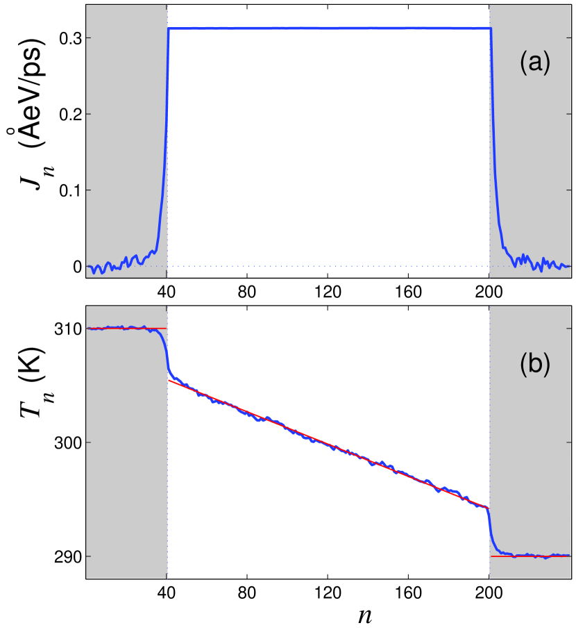
Figure 3: (Color online) Distribution of (a) local heat flux $J_{n}$ and (b) local average temperature $T_{n}$ along ideal zigzag nanoribbon with $K=8$. Length of the nanoribbon is $L=(N-1)h=58.8$ nm ($N=240$, $h=0.246$ nm), and temperatures are $T_{+}=310$ K and $T_{-}=290$ K, the numbers of end segments interacting with the thermostats $N_{\pm}=40$ (corresponding fragments are shown in grey). Heat conductivity is $\kappa=177$ W/mK.

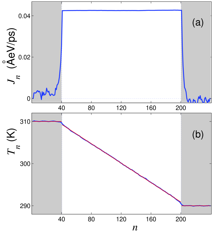
Figure 4: (Color online) Distribution of (a) local heat flux $J_{n}$ and (b) local average temperature $T_{n}$ along a zigzag nanoribbon with rough edges ($K=10$, density $d=0.87$). Length of the nanoribbon is $L=(N-1)h=58.8$ nm ($N=240$, $h=0.246$ nm), and temperatures are $T_{+}=310$ K and $T_{-}=290$ K. Heat conductivity is $\kappa=14$ W/mK.

A linear temperature gradient can be used to define the local coefficient of thermal conductivity, $\kappa(N-N_{+}-N_{-})=(N-N_{-}-N_{+}-1)J/(T_{N_{+}+1}-T_{N-N_{-}})S$, where $S=2(dD_{y}+2r_{C})r_{C}$ is the area of the nanoribbon cross-section (nanoribbon width $D_{y}=(3K/4-1)\rho_{0}$, Van der Waals carbon radius $r_{c}=1.85$Å). Using this definition, we can calculate the asymptotic value of the coefficient $\kappa=\lim_{N\rightarrow\infty}\kappa(N)$.

IV Results

Our analysis of linear eigenmodes of the nanoribbon with periodic boundary conditions in $n$ reveals that in the case of edge disorder almost all vibrational modes are localized as functions of the longitudinal index $n$. This means that in our system we observe the manifestation of the Anderson localization due to the edge disorder, earlier discussed only for the wave transmission in surface-disordered waveguides Freilikher et al. (1990); Sánchez-Gill et al. (1998).

To analyze oscillation eigenmodes, we define the distribution function of the oscillatory energy along the nanoribbon as follows:

$$p_{n}=\sum_{k=1}^{K_{n}}M_{n,k}(|e_{n,k,1}|^{2}+|e_{n,k,2}|^{2}+|e_{n,k,3}|^{2})/M_{0},$$

where $n=1,2,...,N$, $M_{n,k}$ is mass of the atom with the index $(n,k)$, and $\{e_{n,k,i}\}_{i=1}^{3}$ is a component of the corresponding eigenvector (see Ref. Savin and Kivshar (2010a)). The energy distribution is normalized in accord with the condition: $\sum_{n=1}^{N}p_{n}=1.$ To describe the longitudinal energy localization, we introduce a new parameter, $D=1/\sum_{n=1}^{N}p_{n}^{2},$ that characterizes the width of the energy localization along the nanoribbon. If a vibrational mode is localized only on one elementary cell, the corresponding width is $D=1$. In the opposite limit, when the vibrational energy is distributed equally on all elementary cells, we have $D=N$, so that in a general case $1\leq D\leq N$.

Dependence of the width $D$ on the frequency of the oscillatory eigenmodes is shown in Fig. 5. For an ideal nanoribbon, all modes are not localized: when the length $N=300$ we have the width $200\leq D\leq 300$. For nanoribbons with rough edges, only the modes with the wavelength of the order of the nanoribbon length are not localized. As a result, we expect that the edge disorder should lead to suppression of phonon transport and dramatic reduction of the thermal conductivity.

Our numerical results demonstrate that the thermal conductivity of graphene nanoribbon depends crucially on the degree of edge roughness. In spite of the fact that the nanoribbon has an ideal internal structure, its thermal conductivity is reduced dramatically, and it becomes much lower that the conductivity of an ideal nanoribbon of the same width.

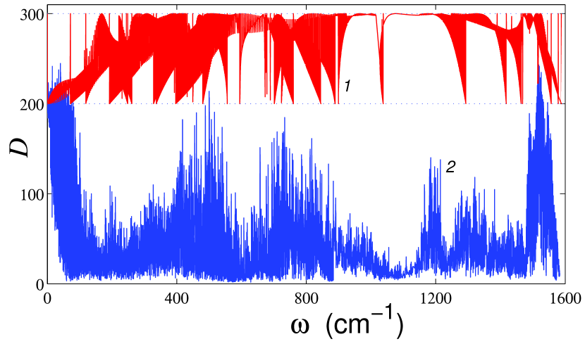
Figure 5: (Color online) Dependence of the width parameter $D$ of linear eigenmodes for the nanoribbon with periodic boundary conditions ($n+N\equiv n$, length $N=300$) on the frequency $\omega$ for an ideal nanoribbon (curve 1, width $K=10$) and a nanoribbon with rough edges (curve 2, $K=10$, $p=0.5$).

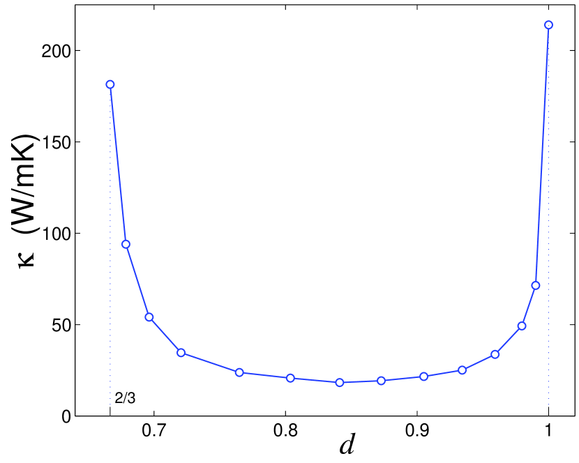
Figure 6: Dependence of the coefficient of thermal conductivity $\kappa$ of a finite nanoribbon with rough edges ($N=240$, $N_{\pm}=40$, $K=12$) on the density $d$.

Distribution of the thermal flow $J_{n}$ and local temperature $T_{n}$ along the ideal nanoribbon and the nanoribbon with rough edges (for the density $d=0.87$) are presented in Figs. 3(a,b) and 4(a,b). In comparison with the ideal nanoribbon, the edge disorder leads to reduction of the thermal flow in at least ten times, as well as it changes the temperature profile along the nanoribbon. In addition, in an ideal nanoribbon we observe thermal resistance at the edges placed into a thermostat, which disappears in the case of rough surfaces. As a result, for the length $L=(N-N_{-}-N_{+})h=39.4$ nm, ($N=240$, $N_{\pm}=40$) the coefficient of thermal conductivity of the nanoribbon with rough edges is found as $\kappa=14$ W/mK that is in 12.6 times lower than the thermal conductivity of an ideal nanoribbon, $\kappa=177$ W/mK.

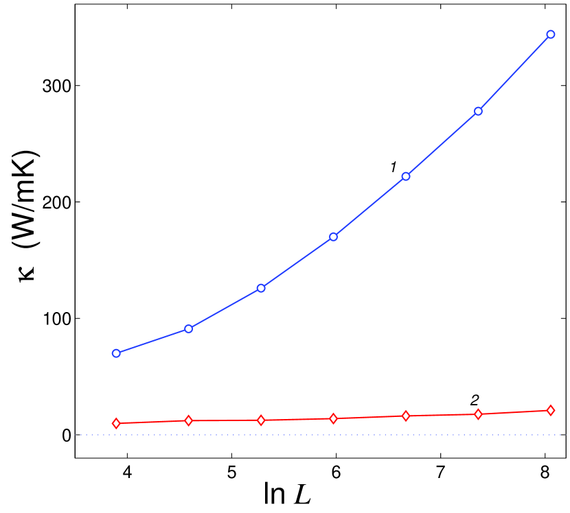
Figure 7: Dependence of the coefficient of thermal conductivity $\kappa$ on the length of the central part of the nanoribbon $L$ (dimension $[L]=$Å). Curve 1 corresponds to an ideal nanoribbon with $K=8$, curve 2 – to edge-disordered nanoribbon with $K=10$, $p=0.5$.

Dependence of the coefficient of thermal conductivity $\kappa$ on the degree of roughness characterized by the parameter $d$ is shown in Fig. 6 for $K=12$, $N=240$, and $N_{\pm}=20$. As follows from this figure, the thermal conductivity will be the lowest for the densities $0.76\leq d<0.93$ (corresponding to the probability of removing the edge atoms, $0.2<p<0.7$). The maximum is observed for $d=1$ (probability $p=0$) and $d=(K-4)/K=2/3$ ($p=1$) when we have ideal nanoribbons with $K=12$ and $K=8$ atoms in an elementary cell, respectively. The minimum is observed for the density $d=0.84$ (probability $p=0.4$). Below, we consider nanoribbons with rough edges created by removing edge atoms with the probability $p=0.5$. The corresponding structure of this nanoribbon is shown in Fig. 2.

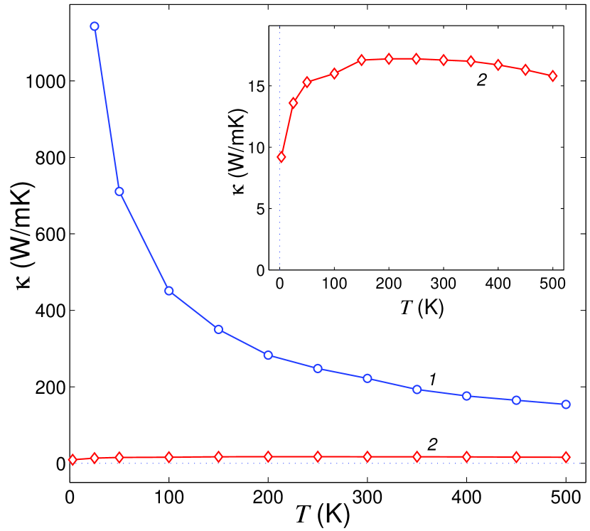
Figure 8: Dependence of the thermal conductivity coefficient $\kappa$ on the temperature $T$ for the ideal finite nanoribbon (curve 1, width $K=8$) and for edge-disordered nanoribbon (curve 2, width $K=10$, probability $p=0.5$). Length of the central part $L=320h=78.6$nm ($N=400$, $N_{\pm}=40$).

Our numerical modeling described above demonstrates that for $T=300$K the thermal conductivity of an ideal nanoribbon grows with its length $L$ as a power-law function, $\kappa\sim L^{\alpha}$ for $L\longrightarrow\infty$ where $\alpha\approx 1/3$. In contrast, the thermal conductivity of a nanoribbon with rough edges grows much slower, see Fig. 7. This difference grows with the length of the nanoribbon. For example, for $L=4.91$ nm $(N=120$, $N_{\pm}=40$), a ratio $\beta$ between the coefficient of thermal conductivity of disordered ($K=12$, $p=0.5$) nanoribbon, $\kappa_{1}$, and ideal ($K=10$, $p=0$) nanoribbon, $\kappa_{0}$, of the same width is $\beta=\kappa_{1}/\kappa_{0}=0.14$, but for the length $L=314.4$ nm this ratio becomes much smaller, $\beta=0.06$.

Efficiency of the thermal conductivity of edge-disordered nanoribbons also decreases with temperature, as well as with the ratio $\beta$. For an ideal nanoribbon, the coefficient of thermal conductivity grows monotonically for low temperatures (see Fig. 8, curve 1), so that for $T\rightarrow 0$ we obtain $\kappa\rightarrow\infty$. This is related to the fact that the dynamics of nanoribbons approached the dynamics of one-dimensional linear system with infinite thermal conductivity. In contrast, for the nanoribbon with rough edges we observe that for $T>100$K its thermal conductivity depends only weakly on temperature, see Fig. 8, curve 2. This result is explained by the fact that in the edge-disordered nanoribbon all linear vibrational modes becomes localized due to the edge disorder, and the phonon transport is suppressed. For low temperatures, the system become linear and its thermal conductivity decays, since a diffusion transport is driven by nonlinear dynamics. As a result, the ratio $\beta=\kappa_{1}/\kappa_{0}$ decays monotonically. For example, for the nanoribbon with the length $L=78.6$ nm, at $T=500$K this ratio is $\beta=0.10$, at $T=300$K, we have $\beta=0.077$, at $T=100$K we obtain $\beta=0.036$, at $T=50$K we find $\beta=0.021$, and at $T=25$K, we have $\beta=0.012$ (i.e. the thermal conductivity is reduced by two orders!).

V Conclusions

We have studied numerically thermal conductivity of carbon nanoribbons with ideal and rough edges. We have demonstrated that thermal conductivity of an ideal nanoribbon is a monotonic power-like function of its length. However, the thermal conductivity is modified dramatically when the structure of nanoribbon edges change. In particular, the thermal conductivity of a nanoribbon with an edge-induced disorder is reduced by several orders of magnitude, and this effect is more pronounced for longer ribbons and low temperatures. As a result, nanoribbons with ideal edges can play a role of highly efficient conductors, while nanoribbons with rough edges become efficient thermal resistors.

References

- Katsnelson (2007) M. I. Katsnelson, Materials Today 10, 20 (2007).
- Lee and Cho (2009) G. Lee and K. Cho, Phys. Rev. B 79, 165440 (2009).
- Engelund et al. (2010) M. Engelund, J. A. Fürst, A. P. Jauho, and M. Brandbyge, Phys. Rev. Lett. 104, 036807 (2010).
- Savin and Kivshar (2010a) A. V. Savin and Y. S. Kivshar, Phys. Rev. B 81, 165418 (2010a).
- Savin and Kivshar (2010b) A. V. Savin and Y. S. Kivshar, EPL 89, 46001 (2010b).
- Evaldsson et al. (2008) M. Evaldsson, I. V. Zozoulenko, H. Xu, and T. Heinzel, Phys. Rev. B 78, 161407(R) (2008).
- Cresti and Roche (2009) A. Cresti and S. Roche, Phys. Rev. B 79, 233404 (2009).
- Martin and Blanter (2009) I. Martin and Y. M. Blanter, Phys. Rev. B 79, 235132 (2009).
- Ghosh et al. (2008) S. Ghosh, I. Calizo, D. Teweldebrhan, E. P. Pokatilov, D. L. Nika, A. A. Balandin, W. Bao, F. Miao, and C. N. Lau, Appl. Phys. Lett. 92, 151911 (2008).
- Balandin et al. (2008) A. A. Balandin, S. Ghosh, W. Bao, I. Calizo, D. Teweldebrhan, F. Miao, and C. N. Lau, Nano Lett. 8, 902 (2008).
- Pop et al. (2006) E. Pop, D. Mann, Q. Wang, K. Goodson, and H. Dai, Nano Lett. 6, 96 (2006).
- Hochbaum et al. (2008) A. L. Hochbaum, R. Chen, R. D. Delgado, W. Liang, E. C. Garnett, M. Najarian, A. Majumdar, and P. Yang, Nature 451, 163 (2008).
- Boukai et al. (2008) A. I. Boukai, Y. Bunimovich, J. Tahir-Kheli, J.-K. Yu, W. A. G. III, and J. R. Heath, Nature 451, 168 (2008).
- Kosevich and Savin (2009) Y. A. Kosevich and A. V. Savin, EPL 88, 14002 (2009).
- Hu et al. (2009) J. Hu, X. Ruan, and Y. P. Chen, Nano Lett. 9, 2730 (2009).
- Noid et al. (1991) D. W. Noid, B. G. Sumpter, and B. Wunderlich, Macromolecules 24, 4148 (1991).
- Savin and Manevitch (2003) A. V. Savin and L. I. Manevitch, Phys. Rev. B 67, 144302 (2003).
- Savin and Kivshar (2008) A. V. Savin and Y. S. Kivshar, Europhys. Letters 82, 66002 (2008).
- Gunlycke et al. (2008) D. Gunlycke, H. M. Lawler, and C. T. White, Phys. Rev. B 77, 014303 (2008).
- Savin et al. (2009) A. V. Savin, B. Hu, and Y. S. Kivshar, Phys. Rev. B 80, 195423 (2009).
- Freilikher et al. (1990) V. D. Freilikher, N. M. Makarov, and I. V. Yurkevich, Phys. Rev. B 41, 8033 (1990).
- Sánchez-Gill et al. (1998) J. A. Sánchez-Gill, V. F. abd I. Yurkevich, and A. A. Maradudin, Phys. Rev. Lett. 80, 948 (1998).