Heat pumping in nanomechanical systems

Abstract

We propose using a phonon pumping mechanism to transfer heat from a cold to a hot body using a propagating modulation of the medium connecting the two bodies. This phonon pump can cool nanomechanical systems without the need for active feedback. We compute the lowest temperature that this refrigerator can achieve.

Freezing out atomic motion by cooling matter to absolute zero temperature is a thought that has, for ages, fascinated both scientists and laymen alike. In atomic gases, techniques such as evaporative cooling can bring temperatures down to the submicrokelvin scale, allowing for the observation of quantum phenomena such as Bose-Einstein condensation. In solid state matter, the ionic motion takes the form of oscillations around equilibrium positions, and completely freezing the system (in the case of an insulator) means removing all lattice vibrations – phonons – leaving solely the quantum mechanical zero-point motion.

The quest for observing quantized mechanical motion in macroscopic systems has incited several experimental groups in recent years sciencereview . In most cases, cooling is obtained by a feedback mechanism which involves optical or electronic sensors and some control system that acts directly on a cantilever. In this Letter, we argue that it is possible to cool a nanomechanical system without relying on feedback control. The mechanism we propose acts directly on the acoustic phonons carrying heat in and out of the system without the need for monitoring its state. By deforming the lattice in the medium connecting the mechanical system to its phonon thermal reservoir, one can pump heat against a temperature gradient by extracting out phonons. The mechanism resembles a classical cooling cycle of a thermal machine and its physical basis is time-reversal symmetry breaking. The pump works in both coherent and incoherent phonon regimes.

Quantum coherent electron pumps have been studied extensively since Thouless’s original proposal thouless83 . For instance, using lateral quantum dots and quantum wires, charge brouwer98 , spin sharma01 , and heat arrachea05 currents can be created in the absence of bias by modulating adiabatically and periodically in time two independent external parameters. In contrast, pumping massless bosons such as acoustic phonons is a much more subtle problem. For one, it is much harder to pump adiabatically phonons due to the lack of a large energy scale such as the Fermi energy. Moreover, phonons not only obey a different wave equation but are also not conserved when scattered by external perturbations that couple linearly to the displacement field (i.e., a driving force). The result in this case is entropy generation in addition to pumping.

In practice on can pump phonons with minimum heat generation by coupling quadratically to the displacement field, either by locally modulating the propagation velocity or by locally applying a pinning potential. An extreme example of a pinning perturbation, which preserves phonon number, is one that imposes Dirichlet boundary conditions to the displacement field at a given point in space. When such a perturbation travels along a quasi-one-dimensional medium, it works as a linear peristaltic pump. Below, we show that this mechanism allows for cooling down the system to a minimum temperature $T_{\rm min}$ which, in one-dimension, is given by the expression

$$T_{\rm min}=\sqrt{\sqrt{\Theta_{B}^{4}+T_{H}^{4}}-\Theta_{B}^{2}},$$ (1)

with $\Theta_{B}=\lambda\sqrt{5v_{B}/2\pi^{3}c}$, where $T_{H}$ is the temperature of the hot thermal reservoir, $\lambda$ is the perturbation strength, $c$ is the phonon velocity, and $v_{B}$ is the barrier speed.

A scheme of the pumping cycle is shown in Fig. 1, where the nanomechanical system to be cooled is represented by the left (cold) side. The local modulation in the phonon velocity or pinning potential works like a moving semireflective barrier to the phonons. In process A$\to$B, the barrier is translated from the cold to the hot side of a cavitylike region. After it reaches the endpoint, another barrierlike perturbation is activated at the opposite side of the cavity (process B$\to$C). Then, in C$\to$A^′, the first barrier is deactivated and phonons from the hot reservoir free expand into the cavity. The procedure is then repeated.

Interesting issues arise out of this simple process of moving a reflective barrier (a “mirror”) for phonons, in particular that of phonon pressure across the barrier. Indeed, a similar process to the one described above was used by Bartoli when he attempted to show the applicability of thermodynamics to electromagnetism and raised the question of radiation pressure bartoli , which in turn inspired Boltzmann in his studies of blackbody radiation boltzmann . The issue of phonon pressure is not trivial (and more subtle than the case of photons) as phonons carry crystal momentum (${\bf q}$) but not obviously physical linear momentum (denoted by ${\bf p}$). The connection between these two forms of momentum requires anharmonicity and is given by ${\bf p}_{\bf q}=\gamma\,d\hbar{\bf q}$, where $\gamma$ is the Grüneisen parameter of the lattice and $d$ denotes the spatial dimension AshcroftMermin ; sorbello ; lee . This impacts the relation between pressure and energy density in a phonon gas; for instance, in the case of a single acoustic mode, the relation takes the simple form $p=-\left(\partial F/\partial V\right)_{T}=\gamma E/V$.

We begin by discussing first the case of a fully reflective barrier. We can treat the problem as a gas of phonons, which we cycle according to Fig. 1. Notice that the barrier does not let heat pass through and the cooling is due to the removal of internal energy from the left-hand side, dumping it into the right-hand side, as explained below.

The expansion $A\to B$ is adiabatic and reversible ($\Delta S_{R,L}=0$, i.e., no heat exchange between left- and right-hand sides). Recalling the standard equation for massless bosons, $dS=dE/T+E\,dV/VTd$, we can relate changes in energy to variations in volume. When the barrier moves to the right, the change in internal energies on the two sides are $E_{L}^{B}=E_{L}^{A}-p_{L}{V_{\rm pipe}}/\gamma d$ and $E_{R}^{B}=E_{R}^{A}+p_{R}{V_{\rm pipe}}/\gamma d$, where ${V_{\rm pipe}}$ is the swept volume. Then, once we insert the other barrier to get to $C$, we redraw the boundary of what $L$ is. The volume of $L$ changes by a factor $(V_{L}-{V_{\rm pipe}})/V_{L}$. So in $C$ we have $E_{L}^{C}=\left(1-\frac{{V_{\rm pipe}}}{V_{L}}\right)E_{L}^{B}$, $E_{R}^{C}=E_{R}^{B}$, and $E_{\rm pipe}^{C}=\frac{{V_{\rm pipe}}}{V_{L}}\;E_{L}^{B}$, where the last energy is the one inside the “pipe”. Then, once the right barrier is removed in going $C\to A^{\prime}$, one redraws the boundary of what $R$ is, so $E_{L}^{A^{\prime}}=E_{L}^{C}$ and $E_{R}^{A^{\prime}}=E_{R}^{C}+E_{\rm pipe}^{C}$.

Putting it all together, we have

$$\Delta E_{L}^{A\to A^{\prime}} = \left(1-\frac{{V_{\rm pipe}}}{V_{L}}\right)\left(E_{L}^{A}-\frac{p_{L}}{\gamma\,d}{V_{\rm pipe}}\right)-E_{L}^{A}$$ (2a)

$$= -\left(e_{L}+\frac{p_{L}}{\gamma\,d}\right){V_{\rm pipe}}+\dots,$$

$$\Delta E_{R}^{A\to A^{\prime}} = \frac{{V_{\rm pipe}}}{V_{L}}\;\left(E_{L}^{A}-\frac{p_{L}}{\gamma\,d}{V_{\rm pipe}}\right)+p_{R}{V_{\rm pipe}}$$ (2b)

$$= \left(e_{L}+\frac{p_{R}}{\gamma\,d}\right){V_{\rm pipe}}+\dots,$$

where $$\dots {V_{\rm pipe}}/V_{L,R} e_{R,L}=E_{R,L}/V_{R,L} A\to B$$ stand for terms down by powers of , and are the intensive energy densities in the two sides. All the work done occurs in and is given by

$$W^{A\to A^{\prime}}=\frac{(p_{R}-p_{L})}{\gamma\,d}\,{V_{\rm pipe}}+\dots,$$ (2c)

where the leading term is insensitive to changes in the pressures $p_{L,R}$ as the volume expands. The unusual relation between work and volume change shown in Eq. (2c) comes from the fact that, in our scheme, volume changes also require an increase in the number of unit cells, so that the lattice unit cell volume is kept constant (i.e., no compression). The work required to add units cells leads to the $\gamma\,d$ factor dividing the pressure difference. (Notice that this factor is absent for photons, since $\gamma=1/d$ follows from ${\bf p}_{\bf q}=\hbar{\bf q}$. In the case of light, there is no undelying lattice system – an “ether” – that needs to be accounted for.) In the process $A\to A^{\prime}$ described above, all entropy increase occurs when the barrier is removed in going $C\to A^{\prime}$, and the second law of thermodynamics is satisfied. From this analysis, we can compute the energy flux out of the left reservoir per unit time of operation of the cycle:

$${\cal J}_{L}^{E}=\left(e_{L}+\frac{p_{L}}{\gamma\,d}\right)\,v_{B},$$ (3)

where $v_{B}$ is the barrier speed. Here we use for total time the duration of the $A\to B$ stroke, assuming that the equilibration in the entropy production part $C\to A^{\prime}$ is fast compared to this time.

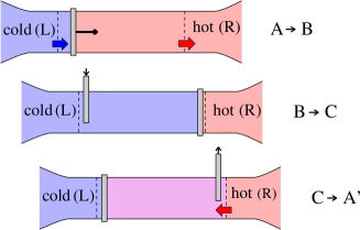
Figure 1: Pumping cycle: A$\rightarrow$B$\rightarrow$C$\rightarrow$A^′ (see text for an explanation). A traveling lattice perturbation acts as a semireflective barrier moving from cold to hot reservoir. The wide arrows indicate unimpeded heat flow.

For our case of interest, $e_{L}=\eta_{d}T_{L}^{d+1}/c^{d}$, where $\eta_{d}=2g\,d!\,\zeta(d+1)/[(4\pi)^{d/2}\Gamma(d/2)]$ with $\zeta(z)$ and $\Gamma(z)$ denoting the Riemann zeta and Gamma functions, respectively, while $g$ is a degeneracy factor. Notice that the energy flux depends only on the intensive quantities for the system on the left (and thus on $T_{L}$), and not on any property on the right-hand side of the barrier, in particular its temperature. This is a straightforward consequence of the fact that the barrier is perfectly reflective, so one is not faced with the difficulty of fighting a thermal gradient between the hot and cold reservoirs. The idealized situation, however, serves the purpose of displaying clearly the main principle of our cooling mechanism.

Let us turn the discussion to the less idealized situation when the barrier is not perfectly reflective, allowing some heat to be transmitted from the hot to the cold side. In this case, we intuitively expect that the slower we move the barrier, the more difficult it becomes to cool, because the energy transferred in the operation $A\to B\to C\to A^{\prime}$ depends only on the volume swept by the barrier, but not on the rate (as long as the $A\to B$ stroke is done in a quasi-equilibrium situation, allowing for thermal equilibration on both sides of the barrier). In addition, the longer we take to move the barrier to the right in the $A\to B$ stroke, the more heat is transferred through the transmitting barrier (the total transfer scales linearly with the sweeping time). So let us now compute the heat flow through the moving barrier, and the conditions to attain net cooling for a semireflective barrier moving with speed $v_{B}$. Hereafter, for simplicity, we focus on a purely one-dimensional case ($d=1$).

For concreteness, consider a “moving mirror” corresponding to a region in space where the atoms are coupled to an external short-range potential, which is localized in space. The position of this pinning potential is modulated in time so as to make it travel at speed $v_{B}$, causing the reflection and transmission coefficients to depend on the red and blue shifted frequencies of the phonons coming from the two reservoirs. Acoustic phonons in a one-dimensional chain, interacting with such a “moving mirror” potential of strength $\lambda$, obey the following wave equation in the continuum limit:

$$\partial_{t}^{2}u(x,t)-c^{2}\partial_{x}^{2}u(x,t)=-\lambda\,c\,\delta(x-v_{B}\,t)\;u(x,t),$$ (4)

It is simpler to work in the reference frame of the barrier, $t^{\prime}=t$ and $x^{\prime}=x-v_{B}t$, where the wave equation becomes

$$\left[\left(\partial_{t^{\prime}}-v_{B}\,\partial_{x^{\prime}}\right)^{2}-c^{2}\partial_{x^{\prime}}^{2}\right]u(x^{\prime},t^{\prime})=-\lambda\,c\,\delta(x^{\prime})\,u(x^{\prime},t^{\prime}).$$ (5)

Let us consider plane wave solutions to Eq. (5) in the two regions, to the left of the barrier (with amplitudes $A_{\omega}^{-}$ and $B_{\omega}^{-}$) and to its right (with $A_{\omega}^{+}$ and $B_{\omega}^{+}$):

$$u_{\pm}(x^{\prime},t^{\prime})=\int\!d\omega\,e^{i\omega t^{\prime}}\left(A^{\pm}_{\omega}e^{-i\omega x^{\prime}/v_{R}}+B^{\pm}_{\omega}e^{i\omega x^{\prime}/v_{L}}\right),$$ (6)

with $v_{R}=c-v_{B}$ and $v_{L}=c+v_{B}$. The function $u(x^{\prime},t^{\prime})$ and its partial time derivatives are continuous, but its partial space derivative is not. Integrating Eq. (5) between $0^{-}$ and $0^{+}$ yields the remaining boundary condition. Matching the solutions on the two sides of the barrier using the boundary conditions yields

$$M_{+}(\omega)\,\left(\begin{array}[]{c}A_{\omega}^{+}\\ B_{\omega}^{+}\end{array}\right) = M_{-}(\omega)\,\left(\begin{array}[]{c}A_{\omega}^{-}\\ B_{\omega}^{-}\end{array}\right)$$ (7e)

where

$$M_{\pm}(\omega)=\left(\begin{array}[]{cc}1&1\\ -i\omega\,v_{L}\mp\lambda\,c/2&i\omega\,v_{R}\mp\lambda\,c/2\end{array}\right)\;.$$ (7f)

Using Eqs. (7e) and (7f), the scattering matrix connecting incoming and outgoing amplitudes can be computed:

$$S(\omega)=\left(\begin{array}[]{cc}\frac{1}{1+i2\,\omega/\lambda}&\frac{i2\,\omega/\lambda}{1+i2\,\omega/\lambda}\\ \frac{-i2\,\omega/\lambda}{1+i2\,\omega/\lambda}&\frac{-1}{1+i2\,\omega/\lambda}\end{array}\right).$$ (8)

Now, to determine the heat transmission and reflection coefficients, one needs to go back to the reference frame of laboratory (i.e., that of the reservoirs), where the Bose-Einstein occupation numbers of the phonons are known: $A_{\omega}^{\pm}=\left(\frac{c}{v_{R}}\right)\,a^{\pm}_{\omega c/v_{R}}$ and $B_{\omega}^{\pm}=\left(\frac{c}{v_{L}}\right)\,b^{\pm}_{\omega c/v_{L}}$, where $\langle{a^{-}_{\omega}}^{\dagger}a^{-}_{\omega}\rangle=n_{L}(\omega)$, $\langle{b^{+}_{\omega}}^{\dagger}b^{+}_{\omega}\rangle=n_{R}(\omega)$, and $\langle{a^{-}_{\omega}}^{\dagger}{b^{+}_{\omega}}\rangle=\langle{b^{+}_{\omega}}^{\dagger}{a^{-}_{\omega}}\rangle=0$, since phonons coming from different reservoirs are uncorrelated. Thus, the heat current leaving the left reservoir is given by the expression

$${\cal J}^{Q}_{L}=\int_{0}^{\infty}d\omega\,\omega\left[n_{L}(\omega)-\langle{b^{-}_{\omega}}^{\dagger}b^{-}_{\omega}\rangle\right].$$ (9)

The quantity $\langle{b^{-}_{\omega}}^{\dagger}b^{-}_{\omega}\rangle$ can be expressed in terms of the distributions $n_{L,R}(\omega)$ through the scattering matrix $S(\omega)$. After a few manipulations, we arrive at

$${\cal J}_{L}^{Q} = \int d\omega\,\omega\left|S_{12}\left(\omega\right)\right|^{2}\left[n_{L}(\omega)-n_{R}(\omega)\right]$$ (10)

$$+ \int d\omega\,\omega\,|S_{11}(\omega)|^{2}\left\{\left[n_{L}(\omega)-\left(\frac{c}{v_{R}}\right)^{2}n_{L}\left(\frac{\omega c}{v_{R}}\right)\right]\right.$$

$$- \left.\left[n_{R}(\omega)-\left(\frac{c}{v_{L}}\right)^{2}n_{R}\left(\frac{\omega c}{v_{L}}\right)\right]\right\}\;.$$

The first line of Eq. (10) is the thermal heat current $I_{\rm thermal}$ from left to right in the presence of a nonmoving barrier. The second line, which we name $I_{\rm pump}$, results from the barrier motion and it is clearly zero when $v_{B}\to 0$ ($v_{L}=v_{R}=c$). In the limit when the barrier amplitude is high, $\lambda\gg T_{R,L}$, we obtain

$${\cal J}_{L}^{Q}\approx\frac{4\pi^{4}}{15}\,\frac{1}{\lambda^{2}c^{2}}\,\left(T_{L}^{4}\,v_{R}^{2}-T_{R}^{4}\,v_{L}^{2}\right).$$ (11)

Notice that this current is always negative if $T_{L}<T_{R}$ and $v_{B}>0$ (with $v_{R}>v_{L}$), thus, as expected, we are fighting this heat flux with the energy flux of Eq. (3). A net flux of energy is indeed possible if we satisfy ${\cal J}_{L}^{E}+{\cal J}_{L}^{Q}>0$, which requires

$$T_{L}^{2} > \frac{4\pi^{3}}{5}\frac{1}{\lambda^{2}cv_{B}}\left(T_{R}^{4}v_{L}^{2}-T_{L}^{4}v_{R}^{2}\right).$$ (12)

As mentioned earlier, for a fully reflective barrier ($\lambda\rightarrow\infty$), cooling can be obtained for any temperature gradient. For a semireflective barrier, to leading order in $v_{B}/c$, cooling requires $T_{L}>T_{\rm min}$, where $T_{\rm min}$ is given by Eq. (1) with $T_{H}=T_{R}$. Notice that when $T_{L}=T_{R}=T$, the proposed mechanism also allows one to transfer heat between reservoirs provided that $T/\lambda<(1/2\pi)\sqrt{5/2\pi}$, independently of the barrier speed.

A few remarks are in order. First, we note that the inequality (12) is independent on $\gamma$. In fact, anharmonicity is not essential for the operation of the cooling mechanism. Although anharmonicity is necessary for equilibration to occur in a closed system, it is not so in an open system coupled to thermal reservoirs. For the latter, equilibration and thermalization takes place over time scales of the order of the time required for sound waves to propagate back and forth through the system. Straightforward numerical simulations of a harmonic linear chain of masses and springs coupled to a thermal reservoir at finite temperature show that, for practical purposes, fast equilibration is achieved when the barrier moves between reservoirs with a speed a few times smaller than $c$. This is important because anharmonic effects are very weak at low temperatures klemens67 ; wolfe98 and should not significantly contribute to equilibration. Second, work is inevitably done when the barriers are activated and deactivated during the $B\to C$ and $C\to A^{\prime}$ processes. However, during a fixed cycle, this work does not scale with the length of the cavity connecting the two reservoirs, while the amount of energy extracted from the cold reservoirs does. Therefore, the contribution of this work to the energy balance of the cooling process can be made very small for a sufficiently long cavity and due to this reason we neglected it in our estimates of the minimum cooling temperature $T_{\rm min}$. Finally, although Eq. (10) has been derived assuming coherent heat transport, Eq. (3) does not rely on quantum coherence. Hence, coherence is not an essential ingredient for our heat pump.

Finally, let us discuss practical implementations. To produce a propagating barrier, it is better to use electromechanical couplings rather than purely mechanical ones, since electronic controlled is both more precise and allows for faster switching times. Strongly electrostrictive materials, in which changes in phonon dispersion are caused by an external electric field, could be used. In particular, electrostrictive polymers such as poly-vinylidene fluoride (PVDF), in which giant electrostriction has been observed zhang98 , appear to be a promising class of materials for building phonon pumps. Like other one-dimensional systems, a single chain of PVDF has four acoustic phonon branches: one longitudinal, two transverse, and one twist mode. Being a highly ionic (or polar) polymer, PVDF has a permanent dipole moment per monomer unit which couples to the external electric field, leading to a gap in the acoustic twist mode dispersion. Therefore a local electric field can virtually block the torsion modes with frequencies below the gap from propagating in PVDF menezes10 , which is equivalent to introducing an infinite barrier for such phonons in our scheme.

In this particular implementation, we can understand more clearly other aspects of the phonon pump. For example, the insertion or removal of the phonon barrier corresponds to turning on or off the electric fields. Because the field causes a phonon gap for the torsional modes, if the insertion is adiabatic, the energy required to do so is given by the phonon energy density that is excluded from the barrier region. As long as the barrier is much narrower than the length of the channel, this energy can be much smaller than the energy pumped as the barrier is pushed along the polymer. In this case, the approximation of neglecting the switching on or off of the barrier (via electric field) holds well. As explained in Ref. menezes10 , for an electric field of 10 MV/cm (a typical field for nanoscale field effect devices), the threshold gap frequency for PVDF corresponds to a temperature of roughly 5 K. Therefore, if the device operates at temperatures below this range, these phonons will be effectively blocked from participating in heat transmission. Coupling PVDF to a grid of backgate electrodes that can be individually controled would effectively produce a moving large barrier potential, as required by our pump. To evaluate the cooling capability of the pump, let us use 5 K as an estimate for $\lambda$ (set by the threshold gap mentioned above) and a velocity ratio $v_{B}/c=1/10$. Then, $\Theta_{B}\approx 0.4$ K; it follows from Eq. (1) that if $T_{H}=100$ mK, $T_{\rm min}\approx 20$ mK, while if $T_{H}=5$ mK, $T_{\rm min}\approx 40$ $\mu$K.

This work is supported in part by the DOE Grant DE-FG02-06ER46316 (CC), CONICET and ANPCyT in Argentina (LA), and CAPES, CNPq, FAPERJ, and INCT-Nanomateriais de Carbono in Brazil (RBC).

References

- (1) For a recent review, see A Cho, Science 327, 516 (2010); O’Connell et al., Nature 464, 697 (2010).
- (2) D. J. Thouless, Phys. Rev. B 27, 6083 (1983).
- (3) P. W. Brouwer, Phys. Rev. B 58, 10135 (1998).
- (4) P. Sharma and C. Chamon, Phys. Rev. Lett. 87, 096401 (2001); E. R. Mucciolo, C. Chamon, and C. M. Marcus, ibid. 89, 146802 (2002).
- (5) M. Moskalets and M. Büttiker, Phys. Rev. B ¡ 66, 035306 (2002); L. Arrachea, M. Moskalets, and L. Martin-Moreno, Phys. Rev. B 75, 245420 (2007); M. Rey et al., Phys. Rev. B 76, 085337 (2007).
- (6) A. Bartoli, Nuovo Cimento 15, 193 (1884); for a historical account, see B. Carazza and H. Kragh, Annals of Science 46, 183 (1989).
- (7) L. Boltzmann, Ann. der Physik 258, 291 (1884).
- (8) N. W. Ashcroft and N. D. Mermin, Solid State Physics (Saunders College, Philadelphia, 1976).
- (9) R. S. Sorbello, Phys. Rev. B 6, 4757 (1972).
- (10) Y. C. Lee and W. Z. Lee, Phys. Rev. B 74, 172303 (2006).
- (11) P. G. Klemens, J. Appl. Phys. 38, 4573 (1967).
- (12) J. P. Wolfe, Imaging Phonons (Cambridge University Press, Cambridge, England, 1998), Ch. 8.
- (13) Q. M. Zhang, V. Bharti, and X. Zhao, Science 280, 2101 (1998).
- (14) M. G. Menezes, A. Saraiva-Souza, J. Del Nero, and R. B. Capaz, Phys. Rev. B 81, 012302 (2010).