The stellar populations of early-type galaxies – I. Observations, line-strengths and stellar population parameters

Abstract

The influence of environment on the formation and evolution of early-type galaxies is, as yet, an unresolved issue. Constraints can be placed on models of early-type galaxy formation and evolution by examining their stellar populations as a function of environment. We present a catalogue of galaxies well suited to such an investigation. The magnitude-limited ($\mathrm{b}_{\mathrm{J}}\lid 19.45$) sample was drawn from four clusters (Coma, A1139, A3558, and A930 at $\left<z\right>=0.04$) and their surrounds. The catalogue contains luminosities, redshifts, velocity dispersions and Lick line strengths for 416 galaxies, of which 245 are classified as early-types. Luminosity-weighted ages, metallicities, and $\alpha$-element abundance ratios have been estimated for 219 of these early-types. We also outline the steps necessary for measuring fully-calibrated Lick indices and estimating the associated stellar population parameters using up-to-date methods and stellar population models. In a subsequent paper we perform a detailed study of the stellar populations of early-type galaxies in clusters and investigate the effects of environment.

1 Introduction

The stellar populations of all but the nearest galaxies are currently unresolvable. Therefore their study relies on the analysis of their integrated light. By examining the absorption lines in an integrated spectrum one can estimate relative luminosity-weighted mean stellar population parameters such as age, metallicity ([Z/H]), and $\alpha$-element abundance ratio ($[\alpha/\mathrm{Fe}]$). The Lick/IDS group defined a system of absorption-line indices that can be used as stellar population tracers (Burstein et al., 1984; Faber et al., 1985; Burstein et al., 1986; Gorgas et al., 1993; Worthey et al., 1994; Trager et al., 1998). These indices can be measured in a consistent way and easily compared to predictions from single stellar population (SSP) models. Recently, synthetic spectra, for the which the stellar population parameters are known, have been used for this purpose (e.g. Vazdekis et al., 2010). When combined with improved methods for estimating $\mathrm{H}\beta$ emission (Sarzi et al., 2006), this appears to be a promising way forward.

Absolute determinations of the stellar population parameters are complicated by the similarity of the effects of age and [Z/H] on a galaxy’s spectral energy distribution, the age–[Z/H] degeneracy (Worthey, 1994), and severely hampered by the effects of the non-solar abundance ratios in early-type galaxies (Worthey, 1996).

Table 1: Details of the clusters from which the galaxy samples were drawn.

Name	R.A.	Dec.	$z$	$\sigma_{clus}$		$N_{z}$		$R_{A}$	B–M
Coma	12 59 48.7	$+27$ 58 50	$0.0232\pm 0.0002$	100	$8\pm 33$	49	9	2	II
A1139	10 58 11.0	$+01$ 36 16	$0.0396\pm 0.0002$	50	$4\pm 47$	10	6	0	III
A3558	13 27 54.0	$-31$ 29 30	$0.0480\pm 0.0003$	97	$7\pm 37$	34	1	4	I
A930	10 07 01.3	$-05$ 37 29	$0.0578\pm 0.0003$	90	$7\pm 82$	9	1	1	III

Coordinates are given in J2000.0. The units of $\sigma_{clus}$ are $\mathrm{kms}^{-1}$; $N_{z}$ is the number of galaxies used to calculate the cluster $z$ and $\sigma_{clus}$.

It is possible to break the age–[Z/H] degeneracy through the use of appropriate absorption-line indices, i.e. by combining an index more sensitive to age variations with one more sensitive to [Z/H] variations (Rabin, 1982; Gonzalez, 1993). By comparing the line-strengths of two (or more) of these indices to predictions from an SSP model through the use of line-diagnostic diagrams, stellar population parameters can be estimated for individual galaxies. It must be stressed that these are relative, luminosity-weighted mean stellar population parameters; a small percentage of recently-formed luminous stars can contribute a disproportionate amount of flux to an integrated spectrum.

In luminous early-type galaxies, it is well known that Mg is observed to be over-abundant relative to Fe when compared with the solar ratio (Peletier, 1989; Worthey et al., 1992; Davies et al., 1993; Fisher et al., 1995; Greggio, 1997; Mehlert et al., 1998; Jørgensen, 1999; Kuntschner, 2000, and others). This leads to indices such as Mgb and Mg₂ yielding higher metallicities and/or younger ages than indices such as Fe5270 and Fe5335, when compared to stellar population models based on solar abundances. Every stellar population model that uses Milky Way-based index calibrations suffers from this bias in $[\alpha/\mathrm{Fe}]$ where indices reflect super-solar $[\alpha/\mathrm{Fe}]$ at sub-solar metallicities (Borges et al., 1995). The current generation of stellar population models, such as those of Thomas et al. (2003) that are used in this study, attempt to correct for this bias.

These models are based on the SSP models of Maraston et al. (2002, see also ) and provide line-strengths for the entire set of Lick indices. These models contain variable abundance ratios with $[\alpha/\mathrm{Fe}]=0.0$, 0.3, 0.5 dex, $[\alpha/\mathrm{Ca}]=-0.1$, 0.0, 0.2, and 0.5 dex, and $[\alpha/\mathrm{N}]=-0.5$ and 0.0 dex. [$\alpha$/Fe] is particularly important since it provides information on the formation time-scale of the stellar population. The models cover ages between 1 and 15 Gyr, metallicities between 0.005 and 3.5 times solar, and are calibrated with Milky Way globular clusters for which the metallicity and [$\alpha$/Fe] are known from independent spectroscopy of individual stars (Puzia et al., 2002).

Since SSP models with variable abundance ratios became available, iterative methods have been devised to take into account the $[\alpha/\mathrm{Fe}]$ of the stellar population when deriving its age and [Z/H] from line-diagnostic diagrams. A more straight-forward method involves the simultaneous fitting of a number of indices to the predictions from a stellar population model using a $\chi^{2}$ technique (Proctor, Forbes & Beasley, 2004). The advantage of this method over the line-diagnostic diagram is that the errors on each index can be taken into account. Using a large number of indices maximises the use of the available data and minimises the impact on derived parameters of imperfect calibration to the Lick system and reduction errors. It is this method that we use to estimate the stellar population parameters for our galaxies.

The outline of the remainder of the paper is as follows. Sample selection, observations and basic reductions are detailed in §2. Redshift ($z$) and velocity dispersion ($\sigma$) measurements, and their errors, are discussed in §3. §4 goes through the steps necessary to measure the strength of absorption lines, fully calibrated to the Lick system, including broadening the spectra and correcting the indices for velocity dispersion broadening. The spectral classification of the galaxies is detailed in §5. Estimation of the stellar population parameters and the effects on these estimates of non-solar abundance ratios are discussed in §6. A summary of the final catalogue and its potential uses are provided in §7.

A Hubble parameter $H_{0}=70\mathrm{kms}^{-1}\mathrm{Mpc}^{-1}$, matter density parameter $\Omega_{M}=0.3$ and dark energy density parameter $\Omega_{\Lambda}=0.7$ are adopted throughout this work.

2 Observations and Data Reductions

2.1 Sample selection

The sample of galaxies observed were drawn from four clusters and their surrounds. The clusters, Coma, A1139, A3558, and A930 with $0.02\la z\la 0.06$, were selected to span the range of Abell richness ($R_{A}$) classes and Bautz–Morgan (B–M) classifications. Coma was also selected to calibrate our data to the Lick system, since it has been studied extensively and has published Lick index line-strengths for its early-type galaxies. Details of the clusters are given in Table 1.

A list of potential targets was created in the following manner. Positions, spectroscopic redshifts, and magnitudes for all galaxies inside the instruments’ fields of view were obtained: for A930 and A1139 these data were obtained from the 2dFGRS database (Colless et al., 2001, 2003), while for A3558 they were obtained from NED for the 2dF observations and from the 6dFGS source catalogue (Jones et al., 2004) for the 6dF observations. $\mathrm{b}_{\mathrm{J}}$ and $\mathrm{r}_{\mathrm{F}}$ magnitudes were obtained for the galaxies selected from NED by cross-correlating with the 6dFGS source catalogue. The magnitude limit of 2dFGRS is $\mathrm{b}_{\mathrm{J}}=19.45$ mag and so we impose this limit on the entire sample. The data on the Coma galaxies were obtained from a catalogue compiled by Moore et al. (2002). There are 135 early-type galaxies in the Moore et al. catalogue, all located within the inner $\sim 1$ Mpc of the cluster. The B-band magnitudes were converted to $\mathrm{b}_{\mathrm{J}}$ magnitudes using the equation found in Blair & Gilmore (1982).

The 6dF fields for A1139 and A930 were not centred on these clusters because they are too close to the edge of the 2dFGRS survey area. Instead, the cluster centre was positioned on one side of the 6dF field, which allowed galaxies at larger cluster-centric radial distances to be observed.

Figure 1: The number of galaxies, as a function of magnitude, that were potential targets (open histogram) and those that were observed (closed histogram). The top row gives these details for the galaxies in the clusters A1139, A3558 and A0930 (from left to right) while the bottom row gives these details for the galaxies in their outskirts.

In compiling the list of potential targets, no consideration was given to morphological type, as that information was not available. Classification of galaxies in the final sample was based on inspection of their spectra (i.e. by spectral type, not morphological type).

To ensure that our potential targets were cluster members (or in the case of the 6dF observations, members of structures associated with the clusters) the samples were trimmed of galaxies outside a $\pm 3\sigma_{\mathrm{clus}}$ slice in redshift space centred on the cluster redshift, where $\sigma_{\mathrm{clus}}$ is the cluster velocity dispersion. This was not done for the galaxies in the Coma field, as they were all confirmed cluster members.

When deciding which targets to observe, the highest priority was given to the brightest galaxies with correspondingly lower priorities to fainter galaxies. This had the dual effect of biasing the sample toward the very bright galaxies in the core of the clusters and ensuring that good S/N was achieved for the greatest number of objects in the sample. Histograms showing the number of potential targets and the number of galaxies actually observed as a function of magnitude are given in Figure 1, where the top row is for cluster galaxies and the bottom row is for galaxies in the cluster outskirts and their surrounds. Coma is not shown here since galaxies form this cluster were selected in a different manner (see above). It is evident from this figure that we were successful in targeting the brightest galaxies in each cluster and in their outskirts.

Stars from the Lick/IDS catalogue (Worthey et al., 1994) were selected as velocity templates for the 2dF (HR6159, HR6770, and HR7317) and 6dF observations (HR2574, HR3145, and HR5888). Details of these six stars are given in Table 2. They were also used as Lick standards along with the Coma cluster galaxies as they could be compared to the published line-strength data of Moore et al. (2002).

Table 2: The stars that were observed as stellar standards.

Name	R.A.	Dec.	$\mathrm{m_{B}}$	Spectral type
HR2574	06 54 11.40	$-12$ 02 19.1	5.54	K4III3
HR3145	08 02 15.94	$+02$ 20 04.5	5.67	K2III1
HR5888	15 50 17.55	$+02$ 11 47.4	6.24	G8III5
HR6159	16 32 36.29	$+11$ 29 16.9	6.33	K4III1
HR6770	18 07 18.36	$+08$ 44 01.9	5.60	G8III2
HR7317	19 19 00.10	$-15$ 32 11.7	7.49	K4III8

Coordinates are given in J2000.0.

2.2 Observing method

Table 3: A summary of the instrumental set-up of 2dF and 6dF.

	2dF	6dF
Telescope	3.9 m AAT	1.2 m UKST
FoV (diameter)	$2^{\circ}$	$5.7^{\circ}$
Grating	300B	580V
	1200B
	1200V
Spectral range	3650–8050 Å	3920–5600 Å
	4590–5730 Å
	4580–5720 Å
Dispersion	4.3 Å$\mathrm{pixel}^{-1}$	1.6 Å$\mathrm{pixel}^{-1}$
	1.1 Å$\mathrm{pixel}^{-1}$
	1.1 Å$\mathrm{pixel}^{-1}$
Instrumental resolution (FWHM)	8.9 Å	5.9 Å
	2.2 Å
	2.2 Å
Number of object fibres	400	150
Number of guide fibres	4	4
Object fibre diameter	140 $\mu\mathrm{m}$ ($2.1\arcsec$)	100 $\mu\mathrm{m}$ ($6.7\arcsec$)
Positioner accuracy	$\sim 20\mu\mathrm{m}$ ($\sim 0.3\arcsec$)	$\sim 10\mu\mathrm{m}$ ($\sim 0.7\arcsec$)
Detector	2 $\times$ thinned Tektronix CCD	Marconi CCD47-10
Size	$1024\times 1024$	$1032\times 1056$
Pixel size	24 $\mu\mathrm{m}$	13 $\mu\mathrm{m}$
Gain	2.8 $e^{-}$ ADU-1	0.6 $e^{-}$ ADU-1
Read-out noise	5.2 $e^{-}$	2.8 $e^{-}$

Galaxies in the four clusters and three standard stars (HR6159, HR6770, and HR7317) were observed with 2dF during the nights of 19–21 April 2002 using the 300B and 1200V gratings. The 300B grating was used to maximise the number of Lick indices that could be measured while the 1200V grating was used to enable accurate redshift and velocity dispersion measurements. There was insufficient time to obtain spectra of the A1139 galaxies with the 1200V grating; these were were subsequently obtained on the night 5 January 2003 using the 1200B grating. The mean S/N per Ångström (calculated at the Mgb index) was 25.6 for the 300B observations; 36.2 for the 1200V observations; and 27.5 for the 1200B observations. Multiple observations were made of each galaxy with exposure times of 1200–1800 s and total exposure times ranged from 1–2 hours for the 300B grating and 2–6 hours for the 1200V/1200B. Exposure times were 3–10 s for the stellar standards, which were taken at the end of every night. Each block of exposures was preceded by an arc exposure and a flat-field exposure, and followed by another arc exposure. Offset-sky exposures of 300 s were taken to aid in sky subtraction. The instrumental set-up of 2dF is detailed in Table 3.

Galaxies in the outskirts of the four clusters and the structures surrounding them, and three standard stars (HR2574, HR3145, and HR5888) were observed with 6dF using the 580V grating during the nights of 6–8 March 2003. The mean S/N per Ångström (calculated at the Mgb index) of the observations was 17.8. Multiple observations of the galaxies were taken with exposure times of 1200 s, while exposures of 5–10 s were taken of the stellar standards at the beginning and end of every night. The total exposure times for each cluster ranged from 2–4 hours. Each block of exposures was preceded by an arc lamp exposure and a quartz lamp exposure for mapping the positions of the spectra on the CCD. The 6dF sample contained galaxies in common with the 2dF sample, but mostly consisted of those in the outer regions of each cluster. The instrumental set-up of 6dF is detailed in Table 3.

2.3 Basic reductions

The data were reduced using dedicated reduction pipelines, 2dfdr (Colless et al., 2001) and 6dfdr (Jones et al., 2004). Basic reduction steps carried out by these programs include bias subtraction, spectrum extraction, flat-fielding, wavelength calibration, fibre throughput determination and correction, and sky subtraction.

The 6dF images were flat-fielded using normalised flat-field images but the 2dF images were not flat-fielded because flexure in the spectrographs, which were mounted at prime focus, means that the flat field spectra are extracted from slightly different pixels to those being calibrated. With both instruments the bias level was determined by taking the median of the over-scan region.

The RMS error of the wavelength calibration for the 2dF spectra was $0.30\pm 0.08$ Å (300B) and $0.09\pm 0.02$ Å (1200B/1200V). For the 6dF spectra it was $0.05\pm 0.02$ Å. In all cases, the accuracy of the fit was better than one-tenth of a pixel.

The method used to calculate the fibre throughput varied. For the 300B 2dF spectra and the 6dF spectra the relative throughput of each fibre was calculated from the flux in the 5577 Å sky-line while for the 1200V and 1200B 2dF spectra, the offset-sky method was used. In all cases, a mean sky spectrum was calculated from the spectra obtained with the sky fibres, which was then subtracted from each spectrum after being scaled to the appropriate throughput value.

For 2dF, the sky subtraction accuracy, measured by the residual light in the sky fibres after sky subtraction, is 3.2% (300B), 5.7% (1200V), and 5.2% (1200B). For 6dF it is 3.0%.

3 Redshifts and Velocity Dispersions

3.1 Redshifts

Redshifts were measured using the program runz (Colless et al., 2001), which cross-correlates the galaxy’s spectrum with numerous spectral templates. The IRAF task rvcorrect was then used to correct the observed redshifts to heliocentric redshifts.

Figure 2: Top left: Comparison of the redshifts measured for galaxies observed with 2dF to those from the literature. The keys to the meaning of each symbol are provided in the top left corner (references are provided in the text). Top right: Histogram of the redshift differences between galaxies observed with 2dF and those in the literature. The dashed curve is the best-fitting Gaussian; the mean and standard deviation are given in the top left corner. The bottom two panels are the same as the top two but are for galaxies observed with 6dF.

The top two panels in Figure 2 show a comparison of the heliocentric redshifts measured for galaxies observed with 2dF to redshifts published in the literature and a histogram of the redshift differences. The dashed curve in the right panel is the best-fitting Gaussian for the differences with the mean and standard deviation given in the top left corner. 778 redshifts were obtained from the literature: 293 of these came from 2dFGRS (Colless et al., 2001), 24 from LCRS (Shectman et al., 1996), 10 from Dale et al. (1997), 141 from Bardelli et al. (1994, 1998), 10 from Teague, Carter & Grey (TCG; 1990), 202 from NFPS (Smith et al., 2004), and 98 from Moore et al. (2002). The agreement between this project and the literature is generally good. However, as can be seen from the histogram, there is a statistically significant offset. This offset is of the order of the precision of our redshift measurements and translates to a spectral shift of $\sim 0.5$ Å. Such a shift will have a minimal impact on the measurement of the Lick indices that have central bandpasses on average 35 Å in width. Therefore, the redshifts were not corrected for this offset.

The bottom two panels of Figure 2 show the equivalent plots for the 6dF data. 266 redshifts of galaxies in and around our four clusters were obtained from the literature: 23 of these redshifts came from Moore et al. (2002), 20 from the CfA redshift survey (CfA; Huchra, Vogeley & Geller, 1999), 123 from 2dFGRS, 17 from LCRS, 36 from 6dFGS (Jones et al., 2004), 41 from the FLASH redshift survey (Kaldare et al., 2003), and 6 from ENACS (Katgert et al., 1998). There is no statistically significant offset between the 6dF data and the literature. For both the 2dF and 6dF observations the dispersion of the differences between the measured redshifts and the literature is $\sim 85\mathrm{kms}^{-1}$.

Figure 3: Left: Comparison of pairs of redshifts measured for galaxies with 2dF and 6dF. Right: Histogram of the redshift differences.

25 galaxies were observed with both 2dF and 6dF and have two reliable redshift estimates and in Figure 3 we compare these estimates. There is a statistically significant offset between the two datasets but again it is less than the precision of our redshift measurements. The dispersion of the differences between the two redshift estimates is $33\mathrm{kms}^{-1}$, which is also of the order of our redshift precision.

3.2 Velocity dispersions

The IRAF task fxcor was used to measure the galaxy velocity dispersions. The stars HR6159, HR6770, and HR7317 were used as velocity templates for cross-correlating with the galaxies observed with 2dF, while HR2574, HR3145, and HR5888 were used for the galaxies observed with 6dF (see Table 2 for details). Each of these stars were observed twice, providing six velocity templates for cross-correlating.

Before the velocity dispersions were measured, each spectrum was processed to ensure as close a match as possible with the template against which it was to be cross-correlated. Each galaxy was de-redshifted using the IRAF task dopcor and the redshift provided by runz. The template spectrum was then re-binned so as to match the dispersion of this de-redshifted spectrum. Both spectra were trimmed so that they contained only the wavelength range in common and broadened to the lowest resolution exhibited by either spectrum, since both 2dF and 6dF have instrumental resolutions that are fibre and wavelength dependent.

The above procedure was carried out on each galaxy/template combination and a velocity dispersion measured. The final velocity dispersion was taken as the mean of those derived from the six templates, weighted by the cross-correlation R-value. The top two panels in Figure 4 compare the measured velocity dispersions to those published in the literature. There are 124 velocity dispersions against which we compare our estimates. Of these literature velocity dispersions, 73 are taken from Moore et al. (2002), 8 from Sánchez-Blázquez et al. (2006), 5 from EFAR (Wegner et al., 1999), and 38 from SMAC (Smith et al., 2000). At low velocity dispersions the agreement is good, but at $\sigma>160\mathrm{kms}^{-1}$ our estimates seem to be greater than those in the literature. This offset is mainly caused by the Moore et al. data. At $\sigma>180\mathrm{kms}^{-1}$ there is an offset between this dataset and ours, with our estimates being on average $\sim 17.6\mathrm{kms}^{-1}$ larger. A similar offset of $\sim 17.4\mathrm{kms}^{-1}$ to the Moore et al. data was found by Sánchez-Blázquez et al. (2006). The right panel shows a histogram of the velocity dispersion differences and the best-fitting Gaussian for the data (dashed curve). The mean and the standard deviation, which are given in the top left corner, indicate that there is a small but significant offset of $\sim 8\mathrm{kms}^{-1}$ and that the dispersion of the differences between the estimates is $\sim 15\mathrm{kms}^{-1}$.

The bottom two panels in Figure 4 are identical to the top two but compare the velocity dispersions measured for galaxies observed with both 2dF and 6dF. We see from the left panel that there is large scatter at lower velocity dispersions possibly due to the lower luminosity, and hence lower S/N, of these galaxies. Another possible reason for the scatter could be the aperture corrections (see Section 4.1.2). While the velocity dispersions have been corrected for the differing aperture sizes, it is possible that at lower velocity dispersions the 6dF fibres subtend a linear distance larger than the diameter of the galaxy resulting in an over-correction to the velocity dispersion, in the sense that the velocity dispersion is larger than it should be. The mean of the best-fitting Gaussian for the velocity dispersion errors shows no significant offset between the two datasets, however the dispersion of the differences is $\sim 25\mathrm{kms}^{-1}$.

3.3 Redshift and velocity dispersion errors

The program runz does not provide any estimate of the error associated with a measured redshift, nor does fxcor provide an estimate of the velocity dispersion error. Following Wegner et al. (1999), we estimate redshift and velocity dispersion errors from detailed Monte Carlo simulations of the measurement process. The procedure used here, which is the same for 2dF and 6dF, determines both the redshift and velocity dispersion errors simultaneously as follows.

For each of the six 2dF stellar templates (there were two spectra for each standard) we created a set of simulated spectra with S/N ranging from 10 to 90 in steps of 10. Each spectrum in the set was then Gaussian broadened to give spectra with dispersions from $60\mathrm{kms}^{-1}$ to $400\mathrm{kms}^{-1}$ in steps of $20\mathrm{kms}^{-1}$. Ten realisations of each of these 972 spectra were then generated with Poisson noise. At a given S/N and Gaussian broadening, each simulated spectrum was cross-correlated with the original spectra from the other two stellar templates giving us 240 redshift and velocity dispersion estimates. The procedures used to prepare the simulated spectra and the templates and the settings used in fxcor were identical to those used in the actual measuring of the redshifts and velocity dispersions. The only difference is that in the actual measurements there was a spectral mismatch between the galaxy spectra and the stellar template. However, at the S/N typical of our data this effect is dominated by the Poisson noise.

Figure 4: Top left: Comparison of the velocity dispersions of the galaxies measured with 2dF and 6dF to those published in literature. The solid line has a slope of unity and the dashed line is our fit to the data. The key to the symbols are shown in the top left corner and references are given in the text. Top right: Histogram of velocity dispersion differences. The dashed curve is the best-fitting Gaussian for the data, the mean and standard deviation are given in the top left corner. The bottom two panels are the same as the top two but compare estimates of the velocity dispersion for galaxies observed with both 2dF and 6dF.

Using the above method, the mean redshift error is $80\mathrm{kms}^{-1}$ and the mean velocity dispersion error is 8%. The measured redshifts, velocity dispersions, and the estimated errors are given in Table 5 of Appendix A.

4 Line-strength Indices

Detailed discussion of the Lick system can be found in any of the references given in Section 1. Some of the original index definitions have been modified and it is the version of the index definitions published in Trager et al. (1998) that is used in this study. We also use the indices $\mathrm{H}\beta_{\mathrm{G}}$, [OIII]₁ and [OIII]₂ as defined in Gonzalez (1993).

To make valid comparisons with other datasets, it is essential that the data are correctly transformed to the Lick system. The Lick system and its associated models (e.g. Worthey, 1994; Vazdekis et al., 1996; Thomas et al., 2003) are calibrated at an instrumental resolution of $\sim 9$ Å FWHM for stellar populations with zero velocity dispersion.

Thus the spectra must be broadened to match the resolution of the Lick system before line-strengths are measured and then a correction must be applied to compensate for the change in index strength caused by the broadening resulting from the velocity dispersion of the stellar population. Generally, the effect of velocity dispersion broadening is to weaken the line-strength, as the absorption line is broadened past the limits of the central bandpass, although the result is actually a complicated combination of effects relating to the movement in the levels of the flanking pseudo-continuum as well as the change in width of the spectral feature.

The final step in transforming the data to the Lick system is to apply a correction to an index if it is offset from literature data calibrated to the Lick system. These systematic offsets can be caused, for example, by continuum shape differences. The index Mg₂ has an offset that is of the order of 0.02 mag and is caused by the fact that the original Lick spectra are not flux-calibrated. The procedures used here to transform the data closely follow those outlined in a number of papers (e.g. Gonzalez, 1993; Fisher et al., 1995; Worthey & Ottaviani, 1997; Trager et al., 1998; Kuntschner, 2000).

The Lick spectra cover the wavelength range 4000–6000 Å and have a mean instrumental FWHM of $\sim 9$ Å, increasing at both ends. The instrumental FWHM of the 2dF and 6dF spectra show similar trends with wavelength as well as a fibre dependence. Thus, it is necessary to perform a wavelength-dependent as well as fibre-dependent broadening. The low-resolution 2dF data were of a comparable or slightly lower resolution than the Lick spectral resolution and as such they were not broadened.

Line-strengths were measured using a program called indexf (Cardiel et al., 1998). indexf is a highly versatile program that allows for the measurement of line-strength indices as well as the estimation of errors and S/N per Å in wavelength-calibrated FITS files. Positive values correspond to lines that are in absorption while negative values correspond to those in emission.

None of the spectra obtained in this project was flux calibrated, so to minimise the effects of continuum shape differences, all spectra had their continuum divided out. A low-order polynomial was fit to the continuum of each spectrum and then this fit was divided out.

For the 2dF galaxies all 21 Lick indices, $\mathrm{H}\beta_{\mathrm{G}}$, [OIII]₁, and [OIII]₂ were measured. For the 6dF galaxies 16 Lick indices (from CN₁ to Fe5406), $\mathrm{H}\beta_{\mathrm{G}}$, [OIII]₁, and [OIII]₂ were measured. However, because these indices need to be corrected for offsets to the Lick system (as mentioned above) and for aperture effects, and because these corrections are not available for all indices, the actual usable indices for the 2dF/6dF galaxies are: C₂4668, $\mathrm{H}\beta$, $\mathrm{H}\beta_{\mathrm{G}}$, Fe5015, Mg₁, Mg₂, Mgb, Fe5270, Fe5335 and Fe5406. Aperture corrections are not available for [OIII]₁, [OIII]₂ but these indices were used only to identify emission-line galaxies.

4.1 Line indices corrections

4.1.1 Velocity dispersion corrections

The Lick system is calibrated for stellar populations with zero velocity dispersion. Correction factors must therefore be calculated and applied once the line-strengths have been measured. The effect of velocity broadening is usually to decrease the strength of the index.

The correction factors were determined by empirically measuring the effect of an increasing velocity dispersion on the measured line-strengths. To do this, the standard stars were broadened out to the Lick resolution, using the method described above, and then broadened further in steps of $50\mathrm{kms}^{-1}$ out to a velocity dispersion of $400\mathrm{kms}^{-1}$. At each step the line-strength of each index was measured. A third-order fit was then made for each index to create a relation for which, given a velocity dispersion, a correction factor can be determined. This correction factor is multiplicative for atomic indices and additive for molecular indices.

4.1.2 Aperture corrections

Figure 5: Offsets between the line-strengths of Coma galaxies measured with 2dF and those found in Moore et al. (2002). The solid line is an offset of zero and the dashed line is the measured offset. The value of the offset and its error, and the scatter about the offset, are given at the top of each panel.

It has been known for a long time that elliptical galaxies exhibit line-strength gradients (e.g. Gorgas & Efstathiou, 1987). Thus, corrections must be applied to our measured line-strengths to account for the different physical sizes subtended by fibres of different diameters on galaxies at different redshifts.

Therefore, all line-strengths and velocity dispersions were corrected to the smallest physical size subtended by any of the fibre/redshift combinations used in this project $\sim 1.0$ kpc, i.e. 2dF fibres ($2.1\arcsec$ in diameter) at the mean redshift of the Coma cluster ($z=0.023$). The average line-strength gradients found in Kuntschner et al. (2002) were used to perform these aperture corrections. Gradients are available for only 9 indices: C₂4668, $\mathrm{H}\beta$, Fe5015, Mg₁, Mg₂, Mgb, Fe5270, Fe5335, Fe5406. So subsequent analysis will include only these indices. We also include $\mathrm{H}\beta_{\mathrm{G}}$ in the analysis because we can use the gradient found for $\mathrm{H}\beta$, which we expect to be the same, to perform the aperture corrections. We note that the gradient for H$\gamma_{\mathrm{A}}$ (0.034) is almost identical that of H$\gamma_{\mathrm{F}}$ (0.033). In any case, no gradient was found for $\mathrm{H}\beta$ and so no correction was applied to either $\mathrm{H}\beta$ or $\mathrm{H}\beta_{\mathrm{G}}$. The form of the correction is identical to that found in Jørgensen (1997). The logarithmic velocity dispersion aperture corrections are applied in a manner identical to the line-strength corrections with $\alpha=-0.04$ (Jørgensen, Franx & Kjaergaard, 1995).

4.2 Calibrating the data

The final step in putting the data on to the Lick system is to compare it with published data already calibrated to the Lick system, taking into account the aperture effects mentioned above, and checking for any offsets. For this purpose, Coma cluster galaxies were observed with both 2dF and 6dF.

Plots of the offsets between our data and that in the literature for all indices for which aperture corrections were applied are shown in Figures 5 and 6. In each panel the solid line represents zero offset while the dashed line represents the mean offset that needs to be added to our data to bring them into agreement with the literature values. Indices with an offset significant at greater than the $3\sigma$ were corrected.

Figure 6: Offsets between the line-strengths of Coma galaxies measured with 6dF and those found in Moore et al. (crosses), and the fully calibrated 2dF data (open circles). The solid line is an offset of zero and the dashed line is the measured offset. The value of the offset and its error, and the scatter about the offset, are given at the top of each panel.

For the 2dF data (Figure 5), we calibrate our data by comparing to that of Moore et al. (2002). Significant offsets were found for C${}_{2}4668$, Fe5015, Mg₁, Mg₂, and Fe5270. For the 6dF data (Figure 6), we compare our data to the Coma cluster galaxies data of Moore et al. as well as our own fully calibrated 2dF data. Including the 2dF data allows us to increase the number of galaxies in the comparison and to check for offsets between the 2dF and 6dF data before combining the data of galaxies in common. Significant offsets were found for C${}_{2}4668$, $\mathrm{H}\beta$, $\mathrm{H}\beta_{\mathrm{G}}$, Mg₂, and Fe5406.

With the exception of C${}_{2}4668$ and Fe5015 (in both the 2dF and 6dF data) the offsets found are all physically small, being on average only 0.024 mag for molecular indices and 0.143 Å for atomic indices. The offset for Fe5406 (6dF data) was determined from just six data points but since all showed an offset in the same direction this offset was still applied. The offsets for $\mathrm{H}\beta_{\mathrm{G}}$ were, within the errors, consistent with those of $\mathrm{H}\beta$ and so we only show the $\mathrm{H}\beta$ offsets.

5 Spectral classification

As this project is primarily focused on the old stellar populations of early-type galaxies, all galaxies that exhibited signs of star formation were excluded from our sample of early-type galaxies. H$\alpha$ and [OIII]$\lambda$5007 Å emission were used to determine whether a galaxy was star-forming or not. Only the 2dF 300B observations had enough wavelength coverage to measure the strength of H$\alpha$, so for the 6dF observations we relied on [OIII]$\lambda$5007 Å alone.

H$\alpha$ emission was determined for galaxies observed with 2dF using the de-blending function in the IRAF task splot. Fitting a Gaussian to these data reveals no offset from zero emission and that our measurement errors are $\sim 1.9$ Å. Galaxies that showed H$\alpha$ emission more than $2\sigma$ from zero, which equates to H$\alpha$ emission less than $-3.8$ Å (lines in emission have negative line-strengths in the Lick system), were removed from our sample.

Even with these galaxies removed there were galaxies remaining that showed signs of significant [OIII]$\lambda$5007 Å emission, as measured by the index [OIII]₂. Statistically, $\mathrm{H}\beta$ emission has been found to correlate with [OIII]$\lambda$5007 Å (Gonzalez, 1993). Galaxies that show signs of [OIII]$\lambda$5007 Å emission will therefore have weaker $\mathrm{H}\beta$ line-strengths (due to nebular $\mathrm{H}\beta$ emission filling in the stellar $\mathrm{H}\beta$ absorption) and thus incorrectly older ages. The usual procedure in these cases is to correct the $\mathrm{H}\beta$ line-strength by subtracting from it a fraction of the [OIII]₂ line-strength. Two fractions have been suggested and used in the literature: 0.7 (Gonzalez, 1993) and 0.6 (Trager et al., 2000a, b). Recently, the use of [OIII]$\lambda$5007 Å emission to correct for $\mathrm{H}\beta$ emission, even in a statistical sense, has been questioned (Nelan et al., 2005). The ratio of emission from these two lines spans a large range and galaxies with little to no $\mathrm{H}\beta$ emission can show significant [OIII]$\lambda$5007 Å emission and vice versa.

Therefore, to be certain that the early-type galaxy sample is free from star-forming galaxies, we also exclude any galaxy that shows significant [OIII]$\lambda$5007 Å emission. Galaxies with an [OIII]₂ index less than $-0.4$ Å were deemed to be star-forming and were therefore excluded from the early-type galaxy sample. This represented a 2$\sigma$ cut for the 2dF data and a 1$\sigma$ cut for the 6dF data.

The fully-calibrated line-strengths and errors are given in Table 6 of Appendix A.

6 Stellar Population Parameters

The stellar population parameters age, [Z/H], and $[\alpha/\mathrm{Fe}]$ were estimated using the $\chi^{2}$ method of Proctor et al. (2004) and comparing our measured line-strengths to the models of Thomas et al. (2003). These models are relatively coarse, predicting line-strengths for stellar populations with ages between 1 Gyr and 15 Gyr, [Z/H] between $-2.25$ dex and 0.67 dex, and $[\alpha/\mathrm{Fe}]$ between 0.0 dex and 0.5 dex. The predictions are made at 1 Gyr intervals in the age, but at a small number of varying intervals in [Z/H] and $[\alpha/\mathrm{Fe}]$. To more accurately determine the stellar population parameters, we interpolate the models to a fine grid providing 378000 individual models, spanning [Z/H]$\sim-1.19-0.59$ (in steps of 0.02 dex), age$\sim 1-15$ Gyr (logarithmically, in steps of 0.02 dex), and [$\alpha$/Fe]$\sim-0.19-0.50$ (in steps of 0.01 dex).

For each galaxy, the stellar population parameters corresponding to the set of predicted line-strengths that produces the smallest $\chi^{2}$ when compared with the observed line-strengths are adopted as the values for that galaxy. As in Proctor et al., indices that differed from the accepted fit by more than three times the RMS scatter about it were rejected. The indices Mg₁ and Mg₂ were found to be problematic and so were excluded from the fitting procedure. Both these indices are very broad and possibly were not calibrated correctly due to our dividing out of the continuum before measuring the line-strengths. Besides, very few galaxies had measured line-strengths for these indices as they were at the limit of our wavelength coverage for 6dF and often were affected by sky-lines. This left a maximum of seven indices with which to perform the fits: C₂4668, $\mathrm{H}\beta$, Fe5015, Mgb, Fe5270, Fe5355 and Fe5406. A fit was only accepted if $\mathrm{H}\beta$ was used and at least two other indices.

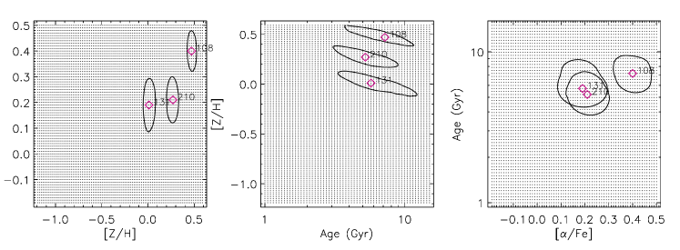
Figure 7: Examples of the confidence limits for the parameter estimates. All three galaxies have roughly mean errors on their indices but span our range in velocity dispersion. One having a low velocity dispersion of $84\mathrm{kms}^{-1}$ (131), one with an average velocity dispersion of $171\mathrm{kms}^{-1}$ (210) and the last with a high velocity dispersion of $299\mathrm{kms}^{-1}$ (108). The grid of dots in each plot represent the models of Thomas et al. (2003) interpolated as described in the text.

Figure 8: The distributions of stellar population parameters for all galaxies in the sample. Marginal distributions are shown for each parameter, and median errors are given in each panel; the dotted lines show the median values of each parameter.

Errors on the parameters were estimated by using the constant $\chi^{2}$ boundaries as confidence limits (see Press et al., 1992). Due to the irregular shape of the grids formed by the stellar population parameters in index space these errors change with position on the grid. Additionally the spacing between lines of constant age reduces when moving to older ages. Therefore the quoted errors for the age estimates are two-sided, but those for the other two parameters are simply the largest of the two errors. As the error estimates cannot be larger than the distance to the edge of the grid this means for some galaxies the positive age errors will be lower limits. Examples of the confidence limits for three galaxies are shown in Figure 7. These galaxies all had roughly mean errors on their indices but were chosen to span our range of velocity dispersions, a low velocity dispersion of $84\mathrm{kms}^{-1}$ (131), one with an average velocity dispersion of $171\mathrm{kms}^{-1}$ (210) and the last with a high velocity dispersion of $299\mathrm{kms}^{-1}$ (108).

The distributions of stellar population parameters for all galaxies in the cluster sample are shown in Figure 8. Marginal distributions are given for each parameter and the dashed line in each denotes the median value. The median [Z/H] is 0.25 dex, the median age 6.3 Gyr, and the median $[\alpha/\mathrm{Fe}]$ is 0.27 dex. Looking at the distribution we see that that they are all roughly Gaussian and that cluster early-type galaxies have mostly super-solar [Z/H], a large spread in age, and $[\alpha/\mathrm{Fe}]$ that mostly falls between 0.2 dex and 0.4 dex. The interpretation of these results, and a discussion of the assumptions made in determining these stellar population parameters, will be the presented in a subsequent paper.

The stellar population parameter estimates and errors are given in Table 7 of Appendix A.

6.1 The effects of $[\alpha/\mathrm{Fe}]$ on stellar population parameter estimates

We now illustrate the problem of estimating ages and [Z/H] without regard to the $[\alpha/\mathrm{Fe}]$ of the population. Using solar-based stellar population models to derive age and [Z/H] estimates results in over-estimated ages and under-estimated [Z/H] if an Fe index is used as the [Z/H] indicator; the opposite will be true if an Mg index is used. More generally, if the model used is based on a single $[\alpha/\mathrm{Fe}]$ then galaxies that have ratios larger than that will have over-estimated ages and under-estimated [Z/H] if using an Fe index as a [Z/H] indicator, and vice versa if an Mg index is used.

Figure 9: The [Z/H] (left) and age (right) residuals as a function of $[\alpha/\mathrm{Fe}]$. In each of the panels the parameter as estimated from the line diagnostic diagram method is subtracted from the parameter as estimated by the $\chi^{2}$ method. $\mathrm{H}\beta$, Mgb, and Fe5335 were used in the $\chi^{2}$ method for all panels while the [Z/H]-sensitive index used in the line diagnostic diagram method was varied: $\langle\mathrm{Fe}\rangle$, Mgb, [MgFe], and [MgFe]^′ (from top to bottom). In all cases $\mathrm{H}\beta$ was used as the age-sensitive index. The dotted vertical line represents the assumed $[\alpha/\mathrm{Fe}]$ for the line diagnostic diagram method.

We illustrate this by comparing our age and [Z/H] estimates from the $\chi^{2}$ method, which has $[\alpha/\mathrm{Fe}]$ as a free parameter, to those derived from line diagnostic diagrams where all galaxies are assumed to have $[\alpha/\mathrm{Fe}]=0.3$ dex. Four different combinations of indices were used; in all cases the age sensitive index was $\mathrm{H}\beta$ and the [Z/H] indicator was one of Mgb, $\langle\mathrm{Fe}\rangle$, [MgFe] (Gonzalez, 1993), or [MgFe]^′ (Thomas et al., 2003) – these latter two indices were designed to be insensitive to $[\alpha/\mathrm{Fe}]$. The resulting differences between the [Z/H] estimated from the four line diagnostic diagrams and the $\chi^{2}$ method as a function of $[\alpha/\mathrm{Fe}]$ are shown in the left panel of Figure 9. The first thing to note is that if the galaxy has an $[\alpha/\mathrm{Fe}]=0.3$ dex then the estimates agree no matter which combination of indices are used. As expected, at $[\alpha/\mathrm{Fe}]>0.3$ dex, $\langle\mathrm{Fe}\rangle$ under-estimates the [Z/H] while Mgb over-estimates it. The opposite is true for each index at $[\alpha/\mathrm{Fe}]<0.3$ dex. For [MgFe] and [MgFe]^′ there is no trend with $[\alpha/\mathrm{Fe}]$, but they consistently under-estimate the [Z/H], with [MgFe]^′ slightly more so than [MgFe].

The right panel of Figure 9 shows the equivalent plots for the age estimates. Again we see that, at $[\alpha/\mathrm{Fe}]=0.3$ dex, all methods agree, but at higher values $\langle\mathrm{Fe}\rangle$ over-estimates the age and Mgb under-estimates it, while the opposite is true at lower values. [MgFe] and [MgFe]^′ consistently over-estimate the ages at $[\alpha/\mathrm{Fe}]<0.3$ dex ([MgFe]^′ slightly more so than [MgFe]) but seem to give reasonable estimates at values greater than this. This exercise emphasises the importance of including $[\alpha/\mathrm{Fe}]$ estimates when estimating ages and [Z/H] of galaxies.

7 Summary

In summary, we have measured velocity dispersions, redshifts and line-strengths for a total of 416 galaxies. These line-strengths were carefully calibrated to the Lick system, and corrected to reflect the strength that would have been obtained using 2dF on galaxies at the redshift of the Coma cluster, i.e. we measured line-strengths of the stellar populations in the inner $\sim 1$ kpc of each galaxy. During the entire process, particular attention was paid to ensuring all sources of errors were properly accounted for.

Table 4: The numbers of galaxies with measured line-strengths and estimated stellar population parameters within the various sub-samples.

Sample	Line-strengths	Parameters
Cluster	158	142
Cluster-outskirts	87	77
Emission-line	168	—
Unclassified	3	—

In a subsequent paper we will explore the variations in the stellar populations of early-type galaxies with redshift and environment using a number of sub-samples defined on our data set – see Table 4. These samples are as follows. 158 are early-type galaxies from Coma, A1139, A3558, or A930 observed with 2dF, 6dF, or both, that are located within the Abell radius (i.e. at a projected radial distance $\leq 2h_{70}^{-1}$ Mpc). This is the cluster sample. 87 are early-type galaxies from the outskirts of these clusters at projected radial distances $>2h_{70}^{-1}$ Mpc. This is the cluster-outskirts sample. 168 galaxies were determined, based on H$\alpha$ and/or [OIII]$\lambda$5007 Å emission, to be star-forming. This is the emission-line sample. The 3 remaining galaxies lacked the information necessary to classify them as either an early-type or emission-line galaxy. We include them in our catalogue because they have measured line-strengths but do not include them in any of the above samples.

Using the fully-calibrated absorption-line indices coupled with the stellar population models of Thomas et al. (2003), we have estimated ages, [Z/H], and $[\alpha/\mathrm{Fe}]$ for 219 galaxies. 142 of these galaxies are in the cluster sample (8 from A930, 8 from A1139, 65 from Coma, and 61 from A3558), and 77 are in the cluster-outskirts sample. In the process we have examined the affect on parameter estimates of non-solar abundance ratios, by comparing various sets of estimates where [$\alpha$/Fe] was fixed to a set of estimates where [$\alpha$/Fe] was a free parameter. We find that the composite indices [MgFe] and [MgFe]^′, although being insensitive to [$\alpha$/Fe], over-estimate ages and under-estimate [Z/H]. The results from this investigation indicate the importance of allowing [$\alpha$/Fe] to be estimated along with [Z/H] and age.

In the second paper of this series we will utilise these data to investigate the stellar populations of early-type galaxies in clusters and their outskirts. Line-strength–$\sigma$ relations will be examined and compared for both the cluster sample and the cluster outskirts sample. Likewise, we will examine and compare the parameter–$\sigma$ relations (i.e. the stellar population parameters) found both in the cluster sample and the cluster outskirts sample. Finally, the intrinsic scatter of the parameter distributions in the cluster sample will be estimated numerically and, combined with the results from parameter–$\sigma$ relations, the degree to which mass and SF time-scale influence the stellar populations of cluster early-type galaxies will be determined. These investigations will provide strong constraints for models of galaxy formation and evolution.

The authors thank the referee, Reynier Peletier, for a careful reading of the paper and for the many helpful suggestions that improved it considerably.

Appendix A Galaxy Catalogues

In this appendix we give the details, line-strengths and stellar population parameters of the galaxies observed as part of this project. Table 5 gives the details of the galaxies such as redshift and velocity dispersion. Column 5 denotes whether the galaxy is considered an early-type galaxy or not, based on H$\alpha$ and/or [OIII]$\lambda$5007 Å emission. Table 6 presents their fully-corrected line-strengths while Table 7 presents the stellar population parameters estimated from them.

Complete versions of these tables can be found on-line.

Table 5: Details of the galaxies. Coordinates are in J2000.0; c$z_{\odot}$ and $\sigma$ units are $\mathrm{kms}^{-1}$. The full version of this table is available electronically.

Cluster	Name	R.A.	Dec.	ET	$\mathrm{m_{b_{J}}}$	$\mathrm{M_{b_{J}}}$	$\mathrm{m_{r_{F}}}$	$\mathrm{M_{r_{F}}}$	c$z_{\odot}$	$\epsilon_{\mathrm{c}z_{\odot}}$	$\sigma$	$\epsilon_{\sigma}$
A930	TGN215Z176	09 57 05.57	$-02$ 33 00.9	y	16.44	-20.88	15.29	-21.86	18071	80	242	14
	TGN153Z276	09 58 05.30	$-04$ 13 09.6	y	16.10	-21.24	14.73	-22.43	19540	79	237	14
	TGN153Z259	09 58 41.64	$-04$ 19 51.8	y	15.92	-21.35	14.68	-22.46	14955	79	201	15
	TGN093Z199	09 59 44.18	$-05$ 22 01.2	y	15.42	-21.87	14.07	-23.07	15854	80	324	10
	TGN093Z079	10 01 25.68	$-04$ 52 12.0	n	16.92	-20.38	15.63	-21.51	16873	78	104	18
	TGN094Z319	10 01 40.38	$-05$ 20 56.5	n	17.00	-20.29	15.76	-21.38	15854	78	138	16
	TGN217Z284	10 01 44.05	$-02$ 13 21.8	y	17.23	-20.09	15.98	-21.17	17982	78	119	17
	TGN154Z324	10 02 15.49	$-04$ 44 41.7	n	16.70	-20.63	15.54	-21.61	19122	79	201	15
	TGN094Z273	10 03 20.66	$-05$ 14 10.0	n	18.44	-18.89	17.16	-19.99	19194	80	122	19
	TGN094Z252	10 03 37.28	$-05$ 06 01.2	n	15.90	-21.40	14.82	-22.32	16604	79	189	15
	TGN094Z244	10 03 43.33	$-04$ 39 44.9	y	17.46	-19.87	16.07	-21.08	18972	79	202	15
	TGN154Z183	10 03 52.99	$-04$ 08 43.9	n	17.09	-20.24	15.91	-21.24	18762	78	121	16
	TGN154Z169	10 04 05.76	$-04$ 22 15.4	y	17.18	-20.15	16.24	-20.91	19062	79	174	17
	TGN217Z071	10 04 11.62	$-02$ 51 12.8	y	16.65	-20.67	15.32	-21.83	18102	80	306	13
	TGN095Z338	10 04 15.24	$-06$ 03 09.0	n	17.16	-20.16	15.93	-21.22	18474	79	137	13
	TGN095Z321	10 04 49.94	$-05$ 11 22.6	n	17.43	-19.85	16.13	-21.01	15566	79	165	11
	TGN094Z172	10 04 50.11	$-05$ 49 36.5	n	17.13	-20.19	15.88	-21.27	18624	78	135	14
	TGN217Z056	10 04 53.59	$-03$ 25 50.1	n	17.31	-19.96	16.11	-21.02	14685	78	155	17
	TGN094Z163	10 04 57.00	$-04$ 47 33.7	y	16.11	-21.22	14.79	-22.36	18822	80	289	11
	TGN094Z153	10 04 58.31	$-05$ 03 09.9	y	16.81	-20.52	15.64	-21.51	18648	56	167	9
	TGN095Z308	10 05 16.24	$-05$ 25 14.8	n	18.97	-18.31	17.67	-19.47	15536	78	112	14
	TGN094Z130	10 05 22.24	$-06$ 06 35.1	n	16.78	-20.51	15.43	-21.71	16436	80	216	8
	TGN094Z119	10 05 28.93	$-05$ 06 10.3	n	15.87	-21.42	14.53	-22.61	15771	56	231	8
	TGN095Z275	10 06 03.80	$-05$ 27 34.8	n	15.68	-21.61	14.57	-22.57	15866	79	152	12
	TGN037Z340	10 06 06.33	$-06$ 28 48.8	n	16.64	-20.65	15.27	-21.87	16436	80	220	8
	TGN095Z262	10 06 28.17	$-05$ 30 08.1	n	17.35	-19.97	16.07	-21.08	18324	78	92	15
	TGN154Z063	10 06 30.40	$-03$ 27 13.3	y	16.70	-20.62	15.51	-21.64	17953	79	206	15
	TGN095Z259	10 06 31.11	$-06$ 16 45.9	y	18.52	-18.81	17.21	-19.94	18684	78	95	15
	TGN217Z184	10 06 31.44	$-02$ 00 51.7	n	17.22	-20.12	15.94	-21.22	19721	79	250	13
	TGN094Z077	10 06 35.21	$-05$ 52 01.0	y	17.35	-19.95	15.95	-21.20	17125	79	181	11
	TGN095Z251	10 06 36.97	$-04$ 53 24.4	y	16.37	-20.91	15.03	-22.11	15506	79	223	10
	TGN095Z242	10 06 39.54	$-05$ 38 36.3	n	16.41	-20.89	15.27	-21.87	16874	78	101	17
	TGN095Z234	10 06 44.95	$-05$ 23 18.0	y	16.45	-20.87	15.08	-22.07	18523	80	314	13
	TGN037Z036	10 06 45.99	$-06$ 18 25.0	n	17.58	-19.75	16.29	-20.86	19134	78	106	14
	TGN217Z005	10 06 49.09	$-03$ 10 05.7	y	17.25	-20.09	15.94	-21.22	19422	80	271	14
	TGN095Z220	10 06 52.30	$-05$ 33 13.0	n	17.29	-20.00	16.05	-21.09	16136	79	167	11
	TGN037Z266	10 06 52.83	$-06$ 26 53.4	y	18.25	-19.07	16.90	-20.25	18084	78	104	14
	TGN037Z263	10 06 55.53	$-06$ 30 41.6	y	19.37	-17.96	18.13	-19.02	19014	78	133	14
	TGN094Z050	10 06 57.91	$-05$ 08 45.1	y	17.89	-19.44	16.59	-20.56	18714	79	191	12
	TGN095Z217	10 06 57.93	$-05$ 47 55.2	n	16.77	-20.54	15.66	-21.49	17335	78	142	12
	TGN095Z208	10 06 59.52	$-05$ 37 34.9	y	17.90	-19.41	16.57	-20.58	17485	79	160	11
	TGN094Z043	10 07 00.48	$-05$ 20 21.5	y	18.47	-18.85	17.13	-20.02	18354	78	113	14
	TGN095Z357	10 07 05.82	$-06$ 23 50.1	y	17.98	-19.34	16.63	-20.52	18534	79	181	11
	TGN095Z200	10 07 06.60	$-05$ 36 11.0	y	19.26	-18.04	17.94	-19.20	16526	78	86	16
	TGN094Z031	10 07 10.79	$-05$ 25 23.4	n	17.27	-20.05	15.95	-21.20	18114	79	156	11
	TGN094Z023	10 07 20.36	$-05$ 17 24.3	n	17.80	-19.52	16.53	-20.62	18054	78	96	15
	TGN095Z191	10 07 20.83	$-05$ 32 59.7	n	16.03	-21.27	14.73	-22.41	16705	80	251	12
	TGN037Z015	10 07 27.54	$-06$ 08 48.5	n	17.35	-19.98	16.03	-21.12	19194	80	247	11
	TGN095Z186	10 07 27.72	$-05$ 27 58.7	y	17.64	-19.65	16.40	-20.74	16466	79	186	12
	TGN095Z177	10 07 30.20	$-04$ 45 01.9	y	16.85	-20.48	15.86	-21.29	18798	56	174	9
	TGN095Z183	10 07 31.41	$-06$ 02 28.4	n	16.66	-20.64	15.39	-21.75	16556	79	171	11
	TGN096Z255	10 07 31.56	$-05$ 58 42.1	n	17.91	-19.41	16.61	-20.54	18624	78	116	14
	TGN155Z244	10 07 33.82	$-04$ 28 07.6	n	16.35	-20.97	15.11	-22.04	18523	79	192	15
	TGN094Z002	10 07 34.31	$-05$ 20 05.4	y	16.70	-20.60	15.63	-21.51	16945	78	106	14
	TGN096Z245	10 07 42.55	$-05$ 34 34.9	n	16.97	-20.33	15.61	-21.53	16714	56	205	9
	TGN095Z154	10 07 53.06	$-04$ 39 28.0	y	16.93	-20.38	15.58	-21.57	17584	56	182	9
	TGN095Z149	10 07 55.70	$-04$ 57 31.9	y	17.86	-19.46	16.49	-20.66	18204	79	169	12
	TGN095Z147	10 08 02.07	$-06$ 01 51.3	y	17.23	-20.09	15.90	-21.25	18624	79	197	10
	TGN095Z148	10 08 02.69	$-06$ 03 12.1	n	17.52	-19.80	16.27	-20.88	18444	78	103	15
	TGN096Z221	10 08 05.17	$-05$ 02 16.4	n	16.97	-20.35	15.67	-21.48	18504	82	183	22
	TGN096Z218	10 08 10.96	$-05$ 01 34.4	y	16.53	-20.79	15.12	-22.03	18468	57	284	8
	TGN095Z135	10 08 12.81	$-06$ 01 40.5	n	17.63	-19.70	16.46	-20.69	18894	78	118	14

Landscape table to go here.

Table 6: Line-strengths of the galaxies. Mg₁ and Mg₂ are in magnitudes all other indices are in Å. The full version of this table is available electronically.

Table 7: Stellar population parameters of the galaxies. Age units are Gyr. $N$ is the number of indices used to estimate the parameters. The full version of this table is available electronically.

Name	Age		$\epsilon^{+}_{\mathrm{age}}$	$\epsilon^{-}_{\mathrm{age}}$	[Z/H]		$\epsilon_{\mathrm{[Z/H]}}$	[$\alpha$/Fe]		$\epsilon_{\mathrm{[}\alpha\mathrm{/Fe]}}$	$N$
TGN215Z176	5.	0	6.9	2.9	0.	07	0.20	0.	50	0.36	3
TGN153Z276	5.	5	4.9	2.6	0.	43	0.14	0.	38	0.14	4
TGN153Z259	15.	0	0.0	3.1	0.	19	0.12	-0.	19	0.09	3
TGN093Z199	5.	0	4.1	1.4	0.	57	0.08	0.	04	0.13	4
TGN093Z079	—		—	—	—		—	—		—	—
TGN094Z319	—		—	—	—		—	—		—	—
TGN217Z284	15.	0	0.0	4.1	-0.	13	0.14	-0.	19	0.16	3
TGN154Z324	—		—	—	—		—	—		—	—
TGN094Z273	—		—	—	—		—	—		—	—
TGN094Z252	—		—	—	—		—	—		—	—
TGN094Z244	7.	5	7.5	4.7	0.	33	0.20	0.	04	0.31	3
TGN154Z183	—		—	—	—		—	—		—	—
TGN154Z169	—		—	—	—		—	—		—	—
TGN217Z071	4.	8	7.2	2.6	0.	05	0.22	0.	16	0.34	3
TGN095Z338	—		—	—	—		—	—		—	—
TGN095Z321	—		—	—	—		—	—		—	—
TGN094Z172	—		—	—	—		—	—		—	—
TGN217Z056	—		—	—	—		—	—		—	—
TGN094Z163	3.	3	1.9	0.8	0.	13	0.08	0.	40	0.15	4
TGN094Z153	14.	3	0.7	5.3	0.	19	0.12	0.	20	0.11	5
TGN095Z308	—		—	—	—		—	—		—	—
TGN094Z130	—		—	—	—		—	—		—	—
TGN094Z119	—		—	—	—		—	—		—	—
TGN095Z275	—		—	—	—		—	—		—	—
TGN037Z340	—		—	—	—		—	—		—	—
TGN095Z262	—		—	—	—		—	—		—	—
TGN154Z063	15.	0	0.0	7.1	-0.	13	0.16	0.	33	0.31	3
TGN095Z259	2.	7	3.0	1.1	0.	27	0.18	0.	41	0.15	5
TGN217Z184	—		—	—	—		—	—		—	—
TGN094Z077	11.	9	3.1	3.3	0.	25	0.08	0.	24	0.08	6
TGN095Z251	6.	0	3.1	2.2	0.	31	0.08	0.	30	0.09	5
TGN095Z242	—		—	—	—		—	—		—	—
TGN095Z234	—		—	—	—		—	—		—	—
TGN037Z036	—		—	—	—		—	—		—	—
TGN217Z005	6.	9	6.2	3.4	0.	03	0.14	0.	50	0.31	3
TGN095Z220	—		—	—	—		—	—		—	—
TGN037Z266	1.	1	0.3	0.1	0.	51	0.20	0.	22	0.13	5
TGN037Z263	10.	4	4.6	6.4	0.	13	0.22	-0.	00	0.32	3
TGN094Z050	9.	1	4.6	3.8	0.	21	0.12	0.	02	0.12	5
TGN095Z217	—		—	—	—		—	—		—	—
GN095Z208	6.	3	3.7	1.9	0.	19	0.08	0.	37	0.09	5
TGN094Z043	5.	0	6.4	2.6	0.	11	0.16	0.	29	0.16	5
TGN095Z357	3.	3	2.4	0.8	0.	55	0.12	0.	39	0.10	5
TGN095Z200	7.	9	6.4	4.6	-0.	05	0.16	0.	39	0.16	5
TGN094Z031	—		—	—	—		—	—		—	—
TGN094Z023	—		—	—	—		—	—		—	—
TGN095Z191	—		—	—	—		—	—		—	—
TGN037Z015	—		—	—	—		—	—		—	—
TGN095Z186	6.	6	4.8	2.0	0.	19	0.10	0.	31	0.09	6
TGN095Z177	4.	5	2.0	1.4	0.	31	0.06	0.	25	0.08	6
TGN095Z183	—		—	—	—		—	—		—	—
TGN096Z255	—		—	—	—		—	—		—	—
TGN155Z244	—		—	—	—		—	—		—	—
TGN094Z002	1.	9	0.6	0.3	0.	23	0.08	0.	25	0.09	6
TGN096Z245	—		—	—	—		—	—		—	—
TGN095Z154	6.	9	3.0	2.5	0.	29	0.08	0.	10	0.09	5
TGN095Z149	5.	0	3.7	2.1	0.	27	0.12	0.	27	0.10	5
TGN095Z147	2.	0	0.6	0.2	0.	29	0.06	0.	20	0.06	6
TGN095Z148	—		—	—	—		—	—		—	—
TGN096Z221	—		—	—	—		—	—		—	—
TGN096Z218	14.	3	0.7	2.9	0.	21	0.06	0.	50	0.03	6
TGN095Z135	—		—	—	—		—	—		—	—

References

- Bardelli et al. (1994) Bardelli S., Zucca E., Vettolani G., Zamorani G., Scaramella R., Collins C. A., MacGillivray H. T., 1994, MNRAS, 267, 665
- Bardelli et al. (1998) Bardelli S., Zucca E., Zamorani G., Vettolani G., Scaramella R., 1998, MNRAS, 296, 599
- Blair & Gilmore (1982) Blair M., Gilmore G., 1982, PASP, 94, 742
- Borges et al. (1995) Borges A. C., Idiart T. P., de Freitas Pacheco J. A., Thevenin F., 1995, AJ, 110, 2408
- Burstein et al. (1984) Burstein D., Faber S. M., Gaskell C. M., Krumm N., 1984, ApJ, 287, 586
- Burstein et al. (1986) Burstein D., Faber S. M., Gonzalez J. J., 1986, AJ, 91, 1130
- Cardiel et al. (1998) Cardiel N., Gorgas J., Cenarro J., Gonzalez J. J., 1998, A&AS, 127, 597
- Colless et al. (2001) Colless M., Dalton G., Maddox S. et al., 2001, MNRAS, 328, 1039
- Colless et al. (2003) Colless, M., Peterson B. A., Jackson C. et al., 2003, preprint (astro-ph/0306581)
- Dale et al. (1997) Dale D. A., Giovanelli R., Haynes M. P., Scodeggio M., Hardy E., Campusano L. E., 1997, AJ, 114, 455
- Davies et al. (1993) Davies R. L., Sadler E. M., Peletier R. F., 1993, MNRAS, 262, 650
- Faber et al. (1985) Faber S. M., Friel E. D., Burstein D., Gaskell C. M., 1985, ApJS, 57, 711
- Fisher et al. (1995) Fisher D., Franx M., Illingworth G., 1995, ApJ, 448, 119
- Gonzalez (1993) González J. J., 1993, PhD thesis, Univ. of California Santa Cruz
- Gorgas & Efstathiou (1987) Gorgas J., Efstathiou G., 1987, in de Zeeuw P. T., ed, Proc. IAU Symp. 127, Structure and Dynamics of Elliptical Galaxies, p. 189
- Gorgas et al. (1993) Gorgas J., Faber S. M., Burstein D., Gonzalez J. J., Courteau S., Prosser C., 1993, ApJS, 86, 153
- Greggio (1997) Greggio L., 1997, MNRAS, 285, 151
- Huchra et al. (1999) Huchra J. P., Vogeley M. S., Geller M. J., 1999, ApJS, 121, 287
- Jones et al. (2004) Jones D. H., Saunders W., Colless M. et al., 2004, MNRAS, 355, 747
- Jørgensen (1997) Jørgensen I., 1997, MNRAS, 288, 161
- Jørgensen (1999) Jørgensen I., 1999, MNRAS, 306, 607
- Jørgensen et al. (1995) Jørgensen I., Franx M., Kjaergaard P., 1995, MNRAS, 276, 1341
- Kaldare et al. (2003) Kaldare R., Colless M., Raychaudhury S., Peterson B. A., 2003, MNRAS, 339, 652
- Katgert et al. (1998) Katgert P., Mazure A., den Hartog R., Adami C., Biviano A., Perea J., 1998, A&AS, 129, 399
- Kuntschner (2000) Kuntschner H., 2000, MNRAS, 315, 184
- Kuntschner et al. (2002) Kuntschner H., Smith R. J., Colless M., Davies R. L., Kaldare R., Vazdekis A., 2002, MNRAS, 337, 172
- Maraston (1998) Maraston C., 1998, MNRAS, 300, 872
- Maraston et al. (2002) Maraston C., Kissler-Patig M., Brodie J., Barmby P., Huchra J., 2002, Ap&SS, 281, 137
- Mehlert et al. (1998) Mehlert D., Saglia R. P., Bender R., Wegner G., 1998, A&A, 332, 33
- Moore et al. (2002) Moore S. A. W., Lucey J. R., Kuntschner H., Colless M., 2002, MNRAS, 336, 382
- Nelan et al. (2005) Nelan J. E., Smith R. J., Hudson M. J., Wegner G. A., Lucey J. R., Moore S. A. W., Quinney S. J., Suntzeff N. B., 2005, ApJ, 632, 137
- Peletier (1989) Peletier R. F., 1989, PhD thesis, Univ. of Groningen
- Press et al. (1992) Press W. H., Teukolsky S. A., Vetterling W. T., Flannery B. P., 1992, Numerical recipes in FORTRAN. The art of scientific computing. Cambridge Univ. Press.
- Proctor et al. (2004) Proctor R. N., Forbes D. A., Beasley M. A., 2004, MNRAS, 355, 1327
- Puzia et al. (2002) Puzia T. H., Saglia R. P., Kissler-Patig M., Maraston C., Greggio L., Renzini A., Ortolani S., 2002, A&A, 395, 45
- Rabin (1982) Rabin D., 1982, ApJ, 261, 85
- Sánchez-Blázquez et al. (2006) Sánchez-Blázquez P., Gorgas J., Cardiel N., González J. J., 2006, A&A, 457, 787
- Sarzi et al. (2006) Sarzi M., Falcón-Barroso J., Davies R. et al., 2006, MNRAS, 366, 1151
- Shectman et al. (1996) Shectman S. A., Landy S. D., Oemler A., Tucker D. L., Lin H., Kirshner R. P., Schechter P. L., 1996, ApJ, 470, 172
- Smith et al. (2000) Smith R. J., Lucey J. R., Hudson M. J., Schlegel D. J., Davies R. L., 2000, MNRAS, 313, 469
- Smith et al. (2004) Smith R. J., Hudson M. J., Nelan J. E. et al, 2004, AJ, 128, 1558
- Teague et al. (1990) Teague P. F., Carter D., Gray P. M., 1990, ApJS, 72, 715
- Thomas et al. (2003) Thomas D., Maraston C., Bender R., 2003, MNRAS, 339, 897
- Trager et al. (1998) Trager S. C., Worthey G., Faber S. M., Burstein D., Gonzalez J. J., 1998, ApJS, 116, 1
- Trager et al. (2000b) Trager S. C., Faber S. M., Worthey G., González J. J., 2000, AJ, 119, 1645
- Trager et al. (2000a) Trager S. C., Faber S. M., Worthey G., González J. J., 2000, AJ, 120, 165
- Vazdekis et al. (1996) Vazdekis A., Casuso E., Peletier R. F., Beckman J. E., 1996, ApJS, 106, 307
- Vazdekis et al. (2010) Vazdekis A., Sánchez-Blázquez P., Falcón-Barroso J., Cenarro A. J., Beasley M. A., Cardiel N., Gorgas J., Peletier R. F., 2010, preprint (arXiv:1004.4439v1)
- Wegner et al. (1999) Wegner G., Colless M., Saglia R. P., McMahan R. K., Davies R. L., Burstein D., Baggley G., 1999, MNRAS, 305, 259
- Worthey (1994) Worthey G., 1994, ApJS, 95, 107
- Worthey (1996) Worthey G., 1996, in Leitherer C., Fritze-von-Alvensleben U., Huchra J., eds, ASP Conf. Ser. Vol. 98, From Stars to Galaxies: the Impact of Stellar Physics on Galaxy Evolution, Astron. Soc. Pac., San Francisco, p. 467
- Worthey & Ottaviani (1997) Worthey G., Ottaviani D. L., 1997, ApJS, 111, 377
- Worthey et al. (1992) Worthey G., Faber S. M., Gonzalez J. J., 1992, ApJ, 398, 69
- Worthey et al. (1994) Worthey G., Faber S. M., Gonzalez J. J., Burstein, D., 1994, ApJS, 94, 687