Global Phase Diagram of the Kondo Lattice: From Heavy Fermion Metals to Kondo Insulators

Abstract

We discuss the general theoretical arguments advanced earlier for the $T=0$ global phase diagram of antiferromagnetic Kondo lattice systems, distinguishing between the established and the conjectured. In addition to the well-known phase of a paramagnetic metal with a “large” Fermi surface (${\rm P_{L}}$), there is also an antiferromagnetic phase with a “small” Fermi surface (${\rm AF_{S}}$). We provide the details of the derivation of a quantum non-linear sigma-model (QNL$\sigma$M) representation of the Kondo lattice Hamiltonian, which leads to an effective field theory containing both low-energy fermions in the vicinity of a Fermi surface and low-energy bosons near zero momentum. An asymptotically exact analysis of this effective field theory is made possible through the development of a renormalization group procedure for mixed fermion-boson systems. Considerations on how to connect the ${\rm AF_{S}}$ and ${\rm P_{L}}$ phases lead to a global phase diagram, which not only puts into perspective the theory of local quantum criticality for antiferromagnetic heavy fermion metals, but also provides the basis to understand the surprising recent experiments in chemically-doped as well as pressurized ${\rm YbRh_{2}Si_{2}}$. We point out that the ${\rm AF_{S}}$ phase still occurs for the case of an equal number of spin-$1/2$ local moments and conduction electrons. This observation raises the prospect for a global phase diagram of heavy fermion systems in the Kondo-insulator regime. Finally, we discuss the connection between the Kondo breakdown physics discussed here for the Kondo lattice systems and the non-Fermi liquid behavior recently studied from a holographic perspective.

PACS numbers:

1 Introduction

Critical phenomenon associated with a second-order phase transition is formulated in terms of Landau’s notion of spontaneous symmetry breaking. Consider an antiferromagnetic transition of a rotationally-invariant spin system. Above the Néel transition temperature, $T>T_{N}$, spins retain the rotational invariance. Below the Néel temperature, $T<T_{N}$, the rotational invariance is spontaneously broken, leading to an antiferromagnetic (AF) state in which the order parameter – the staggered magnetization, ${\bf m}$ – acquires a finite value. Approaching the critical point, the order parameter vanishes but strong spatial fluctuations of the order parameter remain. Indeed, the criticality is characterized by this fluctuating order parameter, ${\bf m}({\bf x})$, and is described by a Ginzburg-Landau theory in $d$-spatial dimensions.

What happens when the Néel temperature is tuned to zero? Hertz formulated the problem in the context of itinerant systems, in which the order parameter ${\bf m}$ is associated with a microscopic magnetic state known as the spin density wave (SDW) ²⁵. Hertz further assumed that the fluctuations of this SDW order parameter are the only critical mode. For any quantum statistical system with Hamiltonian $H$, its partition function, $Z={\rm Tre}^{-\beta H}$, where $\beta\equiv 1/kT$, can be considered as a quantum mechanical evolution operator along imaginary time $-i\tau$, where $\tau$ is defined in the range $(0,\hbar\beta)$ with an associated periodic boundary condition. When $T_{N}$ is nonzero, finite-size effects eventually cut off the fluctuations along the imaginary time axis leaving classical critical behavior associated with the spatial fluctuations of the order parameter. When $T_{N}\rightarrow 0$, on the other hand, the imaginary time axis has an infinite extent. Correspondingly, the critical theory is a quantum Ginzburg-Landau theory of ${\bf m}({\bf x},\tau)$ in $d+z$ dimensions, where $z$ is the dynamic exponent. The temporal fluctuations keep track of the quantum nature of the collective fluctuations, but the degree of freedom itself remains to be ${\bf m}$, the coarse-grained staggered magnetization, which is a classical variable.

In recent years, it has become possible to test this picture of order-parameter fluctuations with the explicit observation of the magnetic quantum critical points (QCPs) in heavy fermion metals ^{61, 30, 19}. At the same time, a large body of theoretical work has emerged on the quantum phase transitions in the Kondo lattice Hamiltonian.

The purpose of this paper is multi-fold. We will first discuss the early theoretical and experimental motivations for the local quantum criticality with a Kondo breakdown. We describe the aspects in which this type of QCP differs from the Landau picture of order-parameter fluctuations, as well as the extensive theoretical developments and the pertinent experimental results. The emphasis here is how the well-established heavy fermion state, a paramagnetic metal with a “large” Fermi surface (${\rm P_{L}}$), can be critically broken down.

We proceed to consider the antiferromagnetically ordered part of the Kondo-lattice phase diagram. Our recent work ^{68, 69} introduced a quantum non-linear sigma-model (QNL$\sigma$M) representation of the Kondo lattice Hamiltonian. An asymptotically exact renormalization-group (RG) analysis establishes the existence of an antiferromagnetic phase with a “small” Fermi surface (${\rm AF_{S}}$). Here, we provide the details of the derivation of this QNL$\sigma$M representation, and describe the RG procedure for this mixed fermion-boson system.

These considerations have lead to a proposal for a global phase diagram ^{52, 68, 53}. This phase diagram puts the studies of local quantum criticality into a larger perspective. In addition, recent experimental work on the Ir- and Co- doped ${\rm YbRh_{2}Si_{2}}$ ¹⁸ have uncovered some surprising varieties of quantum phase transitions in heavy fermion metals. Related observations have appeared in pure ${\rm YbRh_{2}Si_{2}}$ under pressure ⁶⁵ and Ge-doped ${\rm YbRh_{2}Si_{2}}$ ¹². These recent theoretical and experimental works have opened up a new direction for the study of quantum criticality and novel phases in heavy fermion metals.

We also consider the case of heavy fermion systems in the regime of Kondo insulators. We show that the small-Fermi-surface antiferromagnetic phase, ${\rm AF_{S}}$, also exists in the 1+1 filling case. Correspondingly, we propose that tuning a Kondo insulator towards larger RKKY interactions can induce it into an antiferromagnetic or paramagnetic metal with a small Fermi surface.

The focus of this article will be on the theoretical issues. More discussions on the experimental systems, with more references, can be found in a recent article ⁵³ as well as in some of the comprehensive review articles ^{61, 30, 19}.

2 Local quantum criticality and Kondo breakdown from the paramagnetic side

2.1 Kondo breakdown and local quantum criticality

Early indications for the failure of the Hertz picture came from inelastic neutron scattering measurements of the dynamical spin susceptibility $\chi({\bf q},\omega)$. Following initial studies of dynamical scaling in heavy fermion metals ⁴, measurements of $\chi({\bf q},\omega)$ in the heavy fermion compound ${\rm CeCu_{6-x}Au_{x}}$ at the critical concentration $x_{c}\approx 0.1$, show that the order-parameter fluctuations contain an anomalous critical exponent, and display the property of $\omega/T$ scaling ^{46, 45, 62}. Both are properties of an interacting fixed point. By contrast, the SDW QCP description ^{25, 31, 33} of such systems would have an effective dimensionality of $d+z\geq 4$, the upper critical dimension of the quantum Ginzburg-Landau theory, and would correspond to a Gaussian fixed point with essentially mean-field exponents and violation of $\omega/T$ scaling.

These results motivated the theoretical proposal of a new class of QCPs. The key characteristic is the emergence of critical modes which are inherently quantum mechanical. For the Kondo lattice system at hand, these modes are associated with a critical Kondo breakdown. This Kondo breakdown picture was already being considered prior to these experimental developments in some related theoretical models ^{56, 59, 47}. In light of the observed interacting behavior, speculations were put forward ^{57, 8} that the Kondo breakdown underlies the interacting behavior observed in the dynamical spin susceptibility. Soon thereafter, concrete theoretical formulations were advanced ^{54, 10, 55}. The Kondo breakdown picture has subsequently been discussed in related formulations ^{49, 38}.

To put things in perspective, the traditional view of heavy-fermion metals is that the ground state is a Kondo singlet. This is a singlet state formed among all the local moments and all the conduction electrons. This Kondo singlet state does not involve any spontaneous symmetry breaking, but involves a macroscopic order. This is a quantum entangled state. A continuous breakdown of the Kondo entanglement gives rise to the quantum critical modes.

A series of works ^{54, 55, 23, 63, 72, 64, 58, 21, 73, 22} have studied the Kondo breakdown effect within an extended dynamical mean-field theory (EDMFT) ^{56, 60, 7} of the Kondo lattice Hamiltonian. The EDMFT equations have been studied using $\epsilon$-expansion RG procedure and various numerical methods. When the Kondo breakdown occurs at the magnetic QCP, the criticality depends on not only the order-parameter fluctuations but also the new Kondo-breakdown critical modes. Correspondingly, fractional critical exponents and $\omega/T$ scaling arise, in a way that is consistent with the experimentally observed dynamical spin susceptibility.

This local quantum critical picture also has implications for electronic excitations. Kondo resonances carry both spin ($1/2$) and charge ($e$). A Kondo breakdown at the magnetic QCP leads to a jump of the Fermi surface at the magnetic quantum critical point ^{57, 8, 54, 10, 55}, as well as a Kondo-breakdown energy scale, $E_{\rm loc}^{*}$, that continuously goes to zero at the magnetic QCP. Both properties also operate when the Kondo breakdown occurs away from the magnetic QCP ^{57, 54, 55, 49, 38}.

The Fermi surface jump has been probed extensively in several heavy-fermion metals. In ${\rm YbRh_{2}Si_{2}}$, it has been demonstrated that Hall coefficient is dominated by the normal component and therefore probes the Fermi surface ³⁷. At low temperatures, the Hall coefficient displays a rapid crossover as a function of the non-thermal control parameter (a relatively small magnetic field). This crossover extrapolates to a jump at the magnetic QCP in the limit of zero temperature, providing evidence for a jump of the Fermi surface. In ${\rm CeRhIn_{5}}$ ^{36, 27}, evidence for a Fermi surface jump accompanied by a mass divergence has come from measurements of the de Haas-van Alphen effect ⁵¹.

The evidence for a Kondo-breakdown energy scale going to zero at the magnetic quantum critical point has come from the measurements of both the Hall effect ³⁷ and thermodynamic quantities ²⁰.

2.2 Extended dynamical mean field theory of Kondo lattice

The collapse of Kondo effect has been extensively studied from the paramagnetic side. A number of effects come into play: the RKKY interactions promote magnetic order, the Kondo interactions favor Kondo-singlet formation, and the dynamical competition between these two types of interactions are important for the transition. One suitable microscopic approach is the extended dynamical mean-field theory (EDMFT) ^{56, 60, 7}. Here we outline the basic equations and the two type of solutions  ^{54, 55, 23, 72, 63, 21, 73, 22}. A more detailed summary can be found in Ref. ⁵³.

We consider the Kondo lattice model:

$$\mathcal{H} = \mathcal{H}_{f}+\mathcal{H}_{c}+\mathcal{H}_{K}$$ (1)

Here, $\mathcal{H}_{c}=\sum_{\vec{k}\sigma}\epsilon_{\vec{k}}\psi^{\dagger}_{\vec{k}\sigma}\psi_{\vec{k}\sigma}$ describes a band of free conduction $c-$electrons, with a bandwidth $W$. $\mathcal{H}_{K}=\sum_{i}J_{K}{\vec{S}}_{i}\cdot{\vec{s}}_{c,i}$ specifies the Kondo interaction of strength $J_{K}$; here the conduction electron spin $\vec{s}_{c,i}=\frac{1}{2}\sum_{\sigma\sigma^{\prime}}\psi^{\dagger}_{\sigma,i}\vec{\tau}_{\sigma\sigma^{\prime}}\psi_{\sigma^{\prime},i}$, where $\vec{\tau}$ is the vector of Pauli matrices. Finally, $\mathcal{H}_{f}=\frac{1}{2}\sum_{ij}I_{ij}{\vec{S}}_{i}\cdot{\vec{S}}_{j}$ is the magnetic Hamiltonian for the spin-$\frac{1}{2}$ $f-$moments, ${\vec{S}}_{i}$. The strength of the exchange interactions, $I_{ij}$, is characterized by, say, the nearest neighbor value, $I$.

Within EDMFT, the dynamical spin susceptibility and the conduction-electron Green’s function respectively have the forms $\chi({\bf q},\omega)=[I_{{\bf q}}+M(\omega)]^{-1}$, and $G({\bf k},\varepsilon)=[\varepsilon+\mu-\varepsilon_{\bf k}-\Sigma(\varepsilon)]^{-1}$. The correlation functions, $\chi({\bf q},\omega)$ and $G({\bf k},\varepsilon)$, are momentum-dependent. At the same time, the irreducible quantities, $M(\omega)$ and $\Sigma(\varepsilon)$, are momentum-independent. They are determined in terms of a Bose-Fermi Kondo model,

$${\cal H}_{\text{imp}} = J_{K}~{}{\bf S}\cdot{\bf s}_{c}+\sum_{p,\sigma}E_{p}~{}c_{p\sigma}^{\dagger}~{}c_{p\sigma}$$ (2)

$$+\;g\sum_{p}{\bf S}\cdot\left(\boldsymbol{\Phi}_{p}+\boldsymbol{\Phi}_{-p}^{\;\dagger}\right)+\sum_{p}w_{p}\,\boldsymbol{\Phi}_{p}^{\;\dagger}\cdot\boldsymbol{\Phi}_{p}\;.$$

The fermionic ($c_{p\sigma}$) and bosonic ($\boldsymbol{\Phi}_{p}$) baths are determined by self-consistency conditions, which manifest the translational invariance, $\chi_{{loc}}(\omega)=\sum_{\bf q}\chi({\bf q},\omega)$, and $G_{{loc}}(\varepsilon)=\sum_{\bf k}G({\bf k},\varepsilon)$. The $(0+1)$-dimensional quantum impurity problem, Eq. (2), has the following Dyson equations: $M(\omega)=\chi_{0}^{-1}(\omega)+1/\chi_{\rm loc}(\omega)$ and $\Sigma(\varepsilon)=G_{0}^{-1}(\varepsilon)-1/G_{\rm loc}(\varepsilon)$, where $\chi_{0}^{-1}(\omega)=-g^{2}\sum_{p}2w_{p}/(\omega^{2}-w_{p}^{2})$ and $G_{0}(\varepsilon)=\sum_{p}1/(\varepsilon-E_{p})$ are the Weiss fields. The EDMFT formulation allows us to study different degrees of quantum fluctuations as manifested in the spatial dimensionality of these fluctuations. The case of two-dimensional magnetic fluctuations are represented in terms of the RKKY density of states that has a non-zero value at the lower edge, e.g.,

$$\rho_{I}(x)\equiv\sum_{\bf q}\delta(x-I_{\bf q})=(1/{2I})\Theta(I-|x|)\;,$$ (3)

where $\Theta$ is the Heaviside step function. Likewise, three-dimensional magnetic fluctuations are described in terms of a $\rho_{I}(x)$ which vanishes at the lower edge in a square-root fashion, e.g.,

$$\rho_{I}(x)=(2/{\pi I^{2}})\sqrt{I^{2}-x^{2}}\,\Theta(I-|x|)\;.$$ (4)

The reduction of the Kondo-singlet amplitude by the dynamical effects of RKKY interactions among the local moments has been considered in some detail in a number of studies based on EDMFT ^{54, 55, 23, 72, 63, 21, 73, 22}. Irrespective of the spatial dimensionality, this weakening of the Kondo effect is seen through the reduction of the $E_{\mathrm{loc}}^{*}$ scale.

Two classes of solutions emerge depending on whether this Kondo breakdown scale vanishes at the AF QCP. In the case of Eq. (4), $E_{\mathrm{loc}}^{*}$ has not yet been completely suppressed to zero when the AF QCP, $\delta_{c}$, is reached from the paramagnetic side. The quantum critical behavior, at energies below $E_{\mathrm{loc}}^{*}$, falls within the SDW type ^{25, 31, 33}. The zero-temperature dynamical spin susceptibility has the following form:

$$\chi({\bf q},\omega)=\frac{1}{f({\bf q})-ia\omega}\;.$$ (5)

Here $f({\bf q})=I_{\bf q}-I_{\bf Q}$, and is generically $\propto({\bf q}-{\bf Q})^{2}$ as the wavevector ${\bf q}$ approaches the AF ordering wavevector ${\bf Q}$. The QCP is described by a Gaussian fixed point. At non-zero temperatures, a dangerously irrelevant operator invalidates the $\omega/T$ scaling ^{31, 33}.

Another class of solutions corresponds to $E_{\mathrm{loc}}^{*}=0$ already at $\delta_{c}$. It arises in the case of Eq. (3), where the quantum critical magnetic fluctuations are strong enough to suppress the Kondo effect. The solution to the local spin susceptibility has the form

$$\chi({\bf q},\omega)=\frac{1}{f({\bf q})+A\,(-i\omega)^{\alpha}W(\omega/T)}\;.$$ (6)

This expression was derived ^{54, 55} within EDMFT studies, through the aid of an $\epsilon$-expansion approach to the Bose-Fermi Kondo model. At the AF QCP, the Kondo effect itself is critically destroyed. The calculation of the critical exponent $\alpha$ is beyond the reach of the $\epsilon$-expansion. In the Ising-anisotropic case, numerical calculations have found $\alpha\approx 0.7$ ^{23, 21, 73, 22}.

The breakdown of the Kondo effect not only affects magnetic dynamics, but also influences the single-electron excitations. As the QCP is approached from the paramagnetic side, the quasi-particle residue $z_{L}\propto(b^{*})^{2}$, where $b^{*}$ is the strength of a pole in the conduction-electron self-energy $\Sigma$, goes to zero. The large Fermi surface turns critical.

3 Quantum non-linear sigma model representation of the Kondo lattice

The local quantum criticality discussed in the previous section implies a breakdown of the Kondo effect at the magnetic QCP. In order to explore this issue further, we study the Kondo effect deep inside the antiferromagnetic region of the phase diagram. This regime arises when the Kondo coupling is infinitesimal compared to the AF exchange interaction among the local moments, i.e. in the regime

$$J_{K}\ll I\ll W$$ (7)

where $W$ is the width of the conduction electron band.

In the regime specified by Eq. (7), our strategy is to expand the Kondo lattice with respect to the limit of $J_{K}=0$, where the local moments and conduction electrons decouple. The appropriate approach to implement this strategy comprises two steps. First, we introduce a representation of the Kondo lattice Hamiltonian in terms of a Quantum Nonlinear Sigma Model (QNL$\sigma$M). This representation, which results in an effective low-energy field theory containing mixed fermions and bosons, has been introduced in Ref. ⁶⁸; the goal of this section is to provide the details of the derivation. Second, this effective low-energy theory is analyzed asymptotically exactly in terms of an RG method; we will go through this in some detail in the following sections. Related studies have also been pursued in Ref. ³⁵.

3.1 Summary of the mapping

Since an explicit demonstration of the mapping will take a fair amount of space, in this subsection we summarize the essential points. Subsequent subsections will provide the details.

The Kondo lattice Hamiltonian has been specified in Eq. (1). For now, we will consider the electron concentration, $x$ per site, to be such that the Fermi surface of $\mathcal{H}_{c}$ alone does not touch the antiferromagnetic zone boundary. Later, we will discuss the modifications necessary for the more general case.

We expand around the limit $J_{K}=0$, where the local-moment and conduction-electron components are decoupled. We will consider, for simplicity, square or cubic lattices, although our results will be generally valid provided the ground state is a collinear antiferromagnet. $\mathcal{H}_{f}$ can be mapped to a QNL$\sigma$M by standard means ^{24, 6}. The low-lying excitations are concentrated in momentum space near ${\vec{q}}={\vec{Q}}$ (the staggered magnetization) and near ${\vec{q}}={\vec{0}}$ (the total magnetization being conserved):

$$2\vec{S}_{i}\to\eta_{\vec{x}}\vec{n}(\vec{x},\tau)\sqrt{1-\left(2a^{d}\vec{L}(\vec{x},\tau)\right)^{2}}+2a^{d}\vec{L}(\vec{x},\tau)$$ (8)

where $\vec{x}$ labels the position, $\eta_{\vec{x}}=\pm 1$ on even and odd sites, $a$ is the lattice constant, and we have used $S=1/2$. The linear coupling $\vec{n}\cdot\vec{s}_{c}$ cannot connect two points on the Fermi surface and is hence unimportant for low energy physics (such a kinematic constraint has appeared in other contexts, e.g. Ref. ⁴³); see Fig. 1a. The Kondo coupling is then replaced by an effective one, $\vec{S}\cdot\vec{s}_{c}\rightarrow a^{d}\vec{L}\cdot\vec{s}_{c}$, corresponding to forward scattering for the conduction electrons; see Fig. 1a.

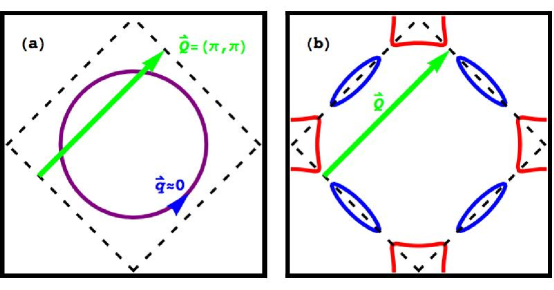
Figure 1: (a) When the Fermi surface of the conduction electrons does not intersect the boundary of the antiferromagnetic Brillouin zone (AFBZ, the dashed lines), the only component of the Kondo coupling to the QNL$\sigma$M fields involves forward scattering for the conduction electrons near the Fermi surface. (b) (from Ref. ⁶⁹) When the Fermi surface of the conduction electrons does not intersect the AFBZ, the Kondo coupling connects the re-diagonalized fermions (whose Fermi surfaces are given by the solid lines) to the QNL$\sigma$M fields. This coupling is also forward scattering in the AFBZ.

The mapping to the QNL$\sigma$M can now be implemented by integrating out the $\vec{L}$ field. The effective action is

$$\mathcal{S} = \mathcal{S}_{\text{QNL}\sigma\text{M}}+\mathcal{S}_{\text{Berry}}+\mathcal{S}_{K}+\mathcal{S}_{c}$$ (9)

$$\mathcal{S}_{\text{QNL}\sigma\text{M}} \equiv \frac{c}{2g}\int d^{d}xd\tau\left[\left(\nabla\vec{n}(\vec{x},\tau)\right)^{2}+\left(\frac{\partial\vec{n}(\vec{x},\tau)}{c~{}\partial\tau}\right)^{2}\right]$$

$$\mathcal{S}_{K} \equiv \lambda\int d^{d}xd\tau\left[\vec{s}_{c}(\vec{x},\tau)\cdot\vec{\varphi}(\vec{x},\tau)\right]$$

$$\mathcal{S}_{c} \equiv \int d^{d}Kd\varepsilon\sum_{\sigma}\psi^{\dagger}_{\sigma}(\vec{K},i\varepsilon)\left(i\varepsilon-\xi_{K}\right)\psi_{\sigma}(\vec{K},i\varepsilon)+\lambda^{2}\int\psi^{4}$$

where $\xi_{K}\equiv v_{F}(K-K_{F})$. The Berry phase term for the $\vec{n}$ field, $\mathcal{S}_{\text{Berry}}$, is not important inside the Néel phase, which is very different from the ferromagnetic case. What is meant by “the Berry phase” requires some clarification. Certainly some aspects of the geometric term do indeed contribute to the physics, but this will be spelled out in the next section. We have introduced a vector boson field $\vec{\varphi}$ which is shorthand for $\vec{n}\times\frac{\partial\vec{n}}{\partial\tau}$. The $\vec{n}$ field satisfies the constraint $\vec{n}^{2}=1$, which is solved by $\vec{n}=(\vec{\pi},\sigma)$, where $\vec{\pi}$ labels the Goldstone magnons and $\sigma\equiv\sqrt{1-\vec{\pi}^{2}}$ is the massive field. We will consider the case of a spherical Fermi surface; since only forward scattering is important, our results will apply for more complicated Fermi-surface geometries. The parameters for the QNL$\sigma$M will be considered as phenomenological ⁶, though they can be explicitly written in terms of the microscopic parameters. The effective Kondo coupling is $\lambda=iJ_{K}/(4dIa^{d})$, which will be explicitly demonstrated below.

This summarizes the structure and setup of the effective field theory for the antiferromagnetic phase of the Kondo lattice model. We now describe the details of how this is done.

3.2 Coherent state representation of the partition function

We set up our notation by considering in some detail the standard case of the Heisenberg model. This will help us perform the analogous mapping for the Kondo lattice model, which is essentially the same but includes conduction electron coupling. We will focus on a square lattice with nearest-neighbor (nn) and next-nearest-neighbor (nnn) spin-exchange interactions, $I_{1}$ and $I_{2}$ respectively.

$$H=\sum_{i,j}I_{ij}\mathbf{S}_{i}\cdot\mathbf{S}_{j}=I_{1}\sum_{\langle ij\rangle}^{nn}\mathbf{S}_{i}\cdot\mathbf{S}_{j}+I_{2}\sum_{\langle\langle ij\rangle\rangle}^{nnn}\mathbf{S}_{i}\cdot\mathbf{S}_{j}=I_{1}\sum_{x,\alpha}\mathbf{S}_{x}\cdot\mathbf{S}_{x+\alpha}+I_{2}\sum_{x,\beta}\mathbf{S}_{x}\cdot\mathbf{S}_{x+\beta}$$

where $x$ runs over all lattice sites, $\alpha$ runs over the nn sites for each lattice site $x$, and $\beta$ runs over nnn sites for each site $x$. After the mapping is completed, it will be clear that the coupling constant $g$ of the QNL$\sigma$M can be tuned by changing $I_{1}$ and $I_{2}$.

The coherent state spin path integral representation of the partition function for quantum spin systems is now a standard formalism that can be found in textbooks (e.g. ^{17, 34}). We will briefly sketch the main idea. The partition function can be written

$$Z = \text{Tr}\;e^{-\beta H}=\lim_{M\rightarrow\infty}\int\mathcal{D}\bm{\Lambda}(\tau)\prod_{k=1}^{M-1}\langle\bm{\Lambda}(\tau_{k+1})\rvert 1-\epsilon H\lvert\bm{\Lambda}(\tau_{k})\rangle$$ (11)

where the many-particle basis is a direct product of single-site spin coherent states: $\lvert\bm{\Lambda}(\tau)\rangle\equiv\prod_{x}\lvert\bm{\Omega}_{x}(\tau)\rangle$. Here $M$ is the number of discrete time slices in the Trotter decomposition, and $\epsilon=\beta/M$. Recall that at each lattice site, $\langle\bm{\Omega}\rvert\mathbf{S}\lvert\bm{\Omega}\rangle=S\bm{\Omega}$, where the unit spin vector is represented by

$$\bm{\Omega}=\frac{1}{\sqrt{S(S+1)}}\mathbf{S}\approx\mathbf{S}/S=(\cos\phi\sin\theta,\sin\phi\sin\theta,\cos\theta).$$

Using this (overcomplete) basis, the matrix elements of the Heisenberg Hamiltonian can thus be written, to leading order in $\epsilon$,

$$\langle\bm{\Lambda}(\tau_{k+1})\rvert H\lvert\bm{\Lambda}(\tau_{k})\rangle = S^{2}\langle\bm{\Lambda}(\tau_{k+1})\rvert\bm{\Lambda}(\tau_{k})\rangle$$

$$\times\left(I_{1}\sum_{x,\alpha}\bm{\Omega}_{x}(\tau_{k})\cdot\bm{\Omega}_{x+\alpha}(\tau_{k})+I_{2}\sum_{x,\beta}\bm{\Omega}_{x}(\tau_{k})\cdot\bm{\Omega}_{x+\beta}(\tau_{k})\right)$$

This allows us to write the Hamiltonian in terms of classical variables $\bm{\Omega}_{x}$. To linear order in $\epsilon$,

$$\langle\bm{\Lambda}(\tau_{k+1})\rvert(1-\epsilon H)\lvert\bm{\Lambda}(\tau_{k})\rangle=\langle\bm{\Lambda}(\tau_{k+1})\rvert\bm{\Lambda}(\tau_{k})\rangle e^{-\epsilon H_{cl}(\tau_{k})}$$ (13)

where

$$H_{cl}(\tau)\equiv S^{2}I_{1}\sum_{x,\alpha}\bm{\Omega}_{x}(\tau)\cdot\bm{\Omega}_{x+\alpha}(\tau)+S^{2}I_{2}\sum_{x,\beta}\bm{\Omega}_{x}(\tau)\cdot\bm{\Omega}_{x+\beta}(\tau)$$ (14)

The penalty for the classical representation is the additional overlap $\langle\bm{\Lambda}(\tau_{k+1})\rvert\bm{\Lambda}(\tau_{k})\rangle$ which is the Berry phase accumulated from the adiabatic evolution from the time-slice $\tau_{k}$ to $\tau_{k+1}$. Including the Berry phase accounts for quantum corrections, and is crucial to obtain the proper mapping to the QNL$\sigma$M. We can write it more clearly as follows:

$$\langle\bm{\Lambda}(\tau_{k+1})\rvert\bm{\Lambda}(\tau_{k})\rangle = \prod_{x,x^{\prime}}\langle\bm{\Omega}_{x}(\tau_{k+1})\rvert\bm{\Omega}_{x^{\prime}}(\tau_{k})\rangle$$ (15)

$$= \prod_{x}\langle\bm{\Omega}_{x}(\tau_{k+1})\rvert\bm{\Omega}_{x}(\tau_{k})\rangle$$

$$= \prod_{x}e^{-iS[1-\cos\theta_{x}(\tau_{k})][\phi_{x}(\tau_{k+1})-\phi_{x}(\tau_{k})]}$$

In the partition function we need an infinite product of such overlaps, which leads to a continuum representation in imaginary time

$$\lim_{M\rightarrow\infty}\prod_{k=1}^{M-1}\langle\bm{\Lambda}(\tau_{k+1})\rvert\bm{\Lambda}(\tau_{k})\rangle = \lim_{M\rightarrow\infty}\prod_{x,k}e^{-iS[1-\cos\theta_{x}(\tau_{k})][\phi_{x}(\tau_{k+1})-\phi_{x}(\tau_{k})]}$$ (16)

$$= \lim_{M\rightarrow\infty}e^{-iS\sum_{x,k}[1-\cos\theta_{x}(\tau_{k})][\phi_{x}(\tau_{k+1})-\phi_{x}(\tau_{k})]}$$

$$= e^{-iS\sum_{x}\int_{0}^{\beta}d\tau[1-\cos\theta_{x}(\tau)]\frac{d\phi_{x}}{d\tau}}$$

$$= e^{-iS\sum_{x}\omega(\bm{\Omega}_{x})}$$

where $\omega(\bm{\Omega}_{x})=\int_{0}^{\beta}d\tau[1-\cos\theta_{x}(\tau)]\frac{d\phi_{x}}{d\tau}$ is the Berry phase for a single spin at site $x$. Note that the total Berry phase contribution to the action in the path integral is given by the sum of the Berry phases of all the lattice site spins: $\mathcal{S}_{B}=iS\sum_{x}\omega(\bm{\Omega}_{x})$. We have represented the Berry phase of a single spin with a set of parameters $\theta_{x}$ and $\phi_{x}$ for familiarity, but we will work with an alternative and convenient representation given by

$$\omega(\bm{\Omega}) = \int_{0}^{\beta}d\tau\int_{0}^{1}du\Bigg{[}\bm{\Omega}(\tau,u)\cdot\frac{\partial\bm{\Omega}(\tau,u)}{\partial u}\times\frac{\partial\bm{\Omega}(\tau,u)}{\partial\tau}\Bigg{]}$$ (17)

where by convention $\bm{\Omega}(\tau,u=1)=\bm{\Omega}(\tau)$ and $\bm{\Omega}(\tau,u=0)=(0,0,1)=\lvert 0\rangle=\lvert S,m=S\rangle$ (see, for example, Ref. ⁴²). $\bm{\Omega}(\tau,u)$ is a homotopically equivalent continuous deformation of $\bm{\Omega}(\tau)$.

Now, in a similar way to what was done above for the Berry phase, we can take the continuum limit to express the Hamiltonian term, $H_{cl}$, as an integration over imaginary time. The partition function then becomes

$$Z = \int\mathcal{D}\bm{\Lambda}(\tau)e^{-\mathcal{S}}$$ (18)

$$\mathcal{S} = \mathcal{S}_{B}+\int_{0}^{\beta}d\tau H_{cl}(\tau)$$ (19)

$$\mathcal{S}_{B} = iS\sum_{x}\int_{0}^{\beta}d\tau\int_{0}^{1}du\Bigg{[}\bm{\Omega}_{x}(\tau,u)\cdot\frac{\partial\bm{\Omega}_{x}(\tau,u)}{\partial u}\times\frac{\partial\bm{\Omega}_{x}(\tau,u)}{\partial\tau}\Bigg{]}$$ (20)

$$H_{cl}(\tau) = S^{2}I_{1}\sum_{x,\alpha}^{nn}\bm{\Omega}_{x}(\tau)\cdot\bm{\Omega}_{x+\alpha}(\tau)+S^{2}I_{2}\sum_{x,\beta}^{nnn}\bm{\Omega}_{x}(\tau)\cdot\bm{\Omega}_{x+\beta}(\tau)$$ (21)

3.3 QNL$\sigma$M mapping for the Heisenberg model

We assume an antiferromagnetic order in which case we can represent each spin as the sum of a staggered component $\mathbf{n}_{x}$ representing the local Néel field, and uniform ($q\approx 0$) fluctuations $\mathbf{L}_{x}$,

$$\bm{\Omega}_{x}(\tau) \equiv \eta_{x}\mathbf{n}_{x}(\tau)\sqrt{1-\left(\frac{a^{d}}{S}\mathbf{L}_{x}(\tau)\right)^{2}}+\frac{a^{d}}{S}\mathbf{L}_{x}(\tau)$$ (22)

The factor $\eta_{x}\in\pm 1$ depending on which sublattice $x$ falls in, while the factor $a^{d}/S$ in front of the uniform fluctuation field $\mathbf{L}$ ensures that integrating around any small volume will yield the total magnetization contained in that volume. Here $a$ is the lattice constant. Recall that the spin variable is constrained by the condition $\bm{\Omega}_{x}\cdot\bm{\Omega}_{x}=1$ at each site. With the above choice, this constraint now becomes $\mathbf{n}_{x}\cdot\mathbf{n}_{x}=1$ and $\mathbf{n}_{x}\cdot\mathbf{L}_{x}=0$. Note that the total number of degrees of freedom in the system remains the same because in the $\mathbf{n}$, $\mathbf{L}$ representation we must restrict ourselves to the antiferromagnetic Brillouin zone (AFBZ); there are twice as many degrees of freedom on half as many sites.

We now wish to write the action in terms of $\mathbf{n}$ and $\mathbf{L}$ rather than $\bm{\Omega}$. We will consider the Berry phase first, then the $H_{cl}$ term.

3.4 Berry phase

Let us first consider what happens when we substitute this expression for the spin into the Berry phase part of the action. We need the expressions for the $\tau$ and $u$ derivatives:

$$\frac{\partial\bm{\Omega}_{x}}{\partial u} \equiv \bm{\Omega}_{u}=\eta\gamma\mathbf{n}_{u}-\frac{\eta}{\gamma}\frac{a^{d}}{S}(\mathbf{L}\cdot\mathbf{L}_{u})\mathbf{n}+\frac{a^{d}}{S}\mathbf{L}_{u}$$ (23)

$$\frac{\partial\bm{\Omega}_{x}}{\partial\tau} \equiv \bm{\Omega}_{\tau}=\eta\gamma\mathbf{n}_{\tau}-\frac{\eta}{\gamma}\frac{a^{d}}{S}(\mathbf{L}\cdot\mathbf{L}_{\tau})\mathbf{n}+\frac{a^{d}}{S}\mathbf{L}_{\tau}$$ (24)

where we temporarily dropped the site index, $x$, and instead use subscripts to denote differentiation. We have also defined $\gamma\equiv\sqrt{1-\left(\frac{a^{d}}{S}\mathbf{L}\right)^{2}}$. Plugging this into equation (20):

$$\mathcal{S}_{B} = iS\sum_{x}\int_{0}^{\beta}d\tau\int_{0}^{1}du\Bigg{[}\left(\eta\gamma\mathbf{n}+\frac{a^{d}}{S}\mathbf{L}\right)\cdot\Big{(}\eta^{2}\gamma^{2}\mathbf{n}_{u}\times\mathbf{n}_{\tau}-\eta^{2}\frac{a^{d}}{S}(\mathbf{L}\cdot\mathbf{L}_{u})\mathbf{n}_{u}\times\mathbf{n}$$

$$+\eta\gamma\frac{a^{d}}{S}\mathbf{n}_{u}\times\mathbf{L}_{\tau}-\eta^{2}\frac{a^{d}}{S}(\mathbf{L}\cdot\mathbf{L}_{u})\mathbf{n}\times\mathbf{n}_{\tau}+\frac{\eta^{2}a^{2d}}{\gamma^{2}S^{2}}(\mathbf{L}\cdot\mathbf{L}_{u})(\mathbf{L}\cdot\mathbf{L}_{\tau})\mathbf{n}\times\mathbf{n}$$

$$-\frac{\eta}{\gamma}\frac{a^{2d}}{S^{2}}(\mathbf{L}\cdot\mathbf{L}_{u})\mathbf{n}\times\mathbf{L}_{\tau}+\eta\gamma\frac{a^{d}}{S}\mathbf{L}_{u}\times\mathbf{n}_{\tau}-\frac{\eta}{\gamma}\frac{a^{2d}}{S^{2}}(\mathbf{L}\cdot\mathbf{L}_{\tau})\mathbf{L}_{u}\times\mathbf{n}+\frac{a^{2d}}{S^{2}}\mathbf{L}_{u}\times\mathbf{L}_{\tau}\Big{)}\Bigg{]}$$

To simplify this equation requires knowing that $\mathbf{n}_{u}$, $\mathbf{n}_{\tau}$ and $\mathbf{L}$ are all perpendicular to $\mathbf{n}$. This means their triple product must vanish: $\mathbf{L}\cdot\mathbf{n}_{u}\times\mathbf{n}_{\tau}=0$. We also neglect terms higher than linear order in $\mathbf{L}$ [terms quadratic in $\mathbf{L}$ are small compared to those kept in Eq. (34)], leading to

$$\mathcal{S}_{B} \approx iS\sum_{x}\int_{0}^{\beta}d\tau\int_{0}^{1}du\Bigg{[}\eta^{3}\gamma^{3}\mathbf{n}\cdot\mathbf{n}_{u}\times\mathbf{n}_{\tau}+\eta^{2}\gamma^{2}\frac{a^{d}}{S}\mathbf{n}\cdot(\mathbf{n}_{u}\times\mathbf{L}_{\tau}+\mathbf{L}_{u}\times\mathbf{n}_{\tau})\Bigg{]}$$

Note also that $\eta_{x}^{2}=1$ and $\eta_{x}^{3}=\eta_{x}$. We then obtain

$$\mathcal{S}_{B} \approx iS\sum_{x}\int_{0}^{\beta}d\tau\int_{0}^{1}du\Bigg{[}\eta\mathbf{n}\cdot\mathbf{n}_{u}\times\mathbf{n}_{\tau}+\frac{a^{d}}{S}\mathbf{n}\cdot(\mathbf{n}_{u}\times\mathbf{L}_{\tau}+\mathbf{L}_{u}\times\mathbf{n}_{\tau})\Bigg{]}$$ (27)

$$= iS\sum_{x}\int_{0}^{\beta}d\tau\int_{0}^{1}du\Bigg{[}\eta_{x}\mathbf{n}_{x}\cdot\frac{\partial\mathbf{n}_{x}}{\partial u}\times\frac{\partial\mathbf{n}_{x}}{\partial\tau}+\frac{a^{d}}{S}\mathbf{n}_{x}\cdot\Bigg{(}\frac{\partial\mathbf{n}_{x}}{\partial u}\times\frac{\partial\mathbf{L}_{x}}{\partial\tau}+\frac{\partial\mathbf{L}_{x}}{\partial u}\times\frac{\partial\mathbf{n}_{x}}{\partial\tau}\Bigg{)}\Bigg{]}$$

$$= iS\sum_{x}\int_{0}^{\beta}d\tau\int_{0}^{1}du\Bigg{[}\eta_{x}\mathbf{n}_{x}\cdot\frac{\partial\mathbf{n}_{x}}{\partial u}\times\frac{\partial\mathbf{n}_{x}}{\partial\tau}+\frac{a^{d}}{S}\frac{\partial}{\partial\tau}\left(\mathbf{n}_{x}\cdot\frac{\partial\mathbf{n}_{x}}{\partial u}\times\mathbf{L}_{x}\right)$$

$$+\frac{a^{d}}{S}\frac{\partial}{\partial u}\left(\mathbf{n}_{x}\cdot\mathbf{L}_{x}\times\frac{\partial\mathbf{n}_{x}}{\partial\tau}\right)\Bigg{]}$$

In the second line we have restored the full notation, while the third line can be written with total derivatives since the terms proportional to $\frac{\partial^{2}\mathbf{n}}{\partial\tau\partial u}$ cancel thanks to the triple product identity $\zeta\cdot\mathbf{b}\times\mathbf{c}=-\mathbf{b}\cdot\zeta\times\mathbf{c}$. The second term in the third line vanishes after integrating the total $\tau$ derivative and using the periodicity of the fields. The third term in the third line can be integrated over $u$, and the value at $u=0$ is zero due to the orthogonality at the north pole. We finally find,

$$\mathcal{S}_{B} = iS\sum_{x}\eta_{x}\int_{0}^{\beta}d\tau\int_{0}^{1}du\left(\mathbf{n}_{x}\cdot\frac{\partial\mathbf{n}_{x}}{\partial u}\times\frac{\partial\mathbf{n}_{x}}{\partial\tau}\right)-i\sum_{x}a^{d}\int_{0}^{\beta}d\tau\left(\mathbf{L}_{x}\cdot\mathbf{n}_{x}\times\frac{\partial\mathbf{n}_{x}}{\partial\tau}\right)$$

The first term is precisely the Berry phase for the Néel component $\mathbf{n}$, while the second term is something additional that must be added to the total action. Although both terms came from the expression for the Berry phase of $\bm{\Omega}$, it is only the first term that is often referred to as the Berry phase for the antiferromagnet.

3.5 Hamiltonian

Next we compute the contribution to the action from the Hamiltonian $H_{cl}(\tau)$ expressed in terms of $\mathbf{n}$ and $\mathbf{L}$ fields. Plugging (22) into (21),

$$H_{cl}(\tau) = S^{2}I_{1}\sum_{x,\alpha}^{nn}\Bigg{[}\eta_{x}\mathbf{n}_{x}(\tau)\sqrt{1-\left(\frac{a^{d}}{S}\mathbf{L}_{x}(\tau)\right)^{2}}+\frac{a^{d}}{S}\mathbf{L}_{x}(\tau)\Bigg{]}$$

$$\cdot\Bigg{[}\eta_{x+\alpha}\mathbf{n}_{x+\alpha}(\tau)\sqrt{1-\left(\frac{a^{d}}{S}\mathbf{L}_{x+\alpha}(\tau)\right)^{2}}+\frac{a^{d}}{S}\mathbf{L}_{x+\alpha}(\tau)\Bigg{]}$$

$$+S^{2}I_{2}\sum_{x,\beta}^{nnn}\Bigg{[}\eta_{x}\mathbf{n}_{x}(\tau)\sqrt{1-\left(\frac{a^{d}}{S}\mathbf{L}_{x}(\tau)\right)^{2}}+\frac{a^{d}}{S}\mathbf{L}_{x}(\tau)\Bigg{]}$$

$$\cdot\Bigg{[}\eta_{x+\beta}\mathbf{n}_{x+\beta}(\tau)\sqrt{1-\left(\frac{a^{d}}{S}\mathbf{L}_{x+\beta}(\tau)\right)^{2}}+\frac{a^{d}}{S}\mathbf{L}_{x+\beta}(\tau)\Bigg{]}$$

$$\approx S^{2}I_{1}\sum_{x,\alpha}^{nn}\Bigg{[}\eta_{x}\mathbf{n}_{x}(\tau)\left(1-\frac{1}{2}\left(\frac{a^{d}}{S}\mathbf{L}_{x}(\tau)\right)^{2}\right)+\frac{a^{d}}{S}\mathbf{L}_{x}(\tau)\Bigg{]}$$

$$\cdot\Bigg{[}\eta_{x+\alpha}\mathbf{n}_{x+\alpha}(\tau)\left(1-\frac{1}{2}\left(\frac{a^{d}}{S}\mathbf{L}_{x+\alpha}(\tau)\right)^{2}\right)+\frac{a^{d}}{S}\mathbf{L}_{x+\alpha}(\tau)\Bigg{]}$$

$$+S^{2}I_{2}\sum_{x,\beta}^{nnn}\Bigg{[}\eta_{x}\mathbf{n}_{x}(\tau)\left(1-\frac{1}{2}\left(\frac{a^{d}}{S}\mathbf{L}_{x}(\tau)\right)^{2}\right)+\frac{a^{d}}{S}\mathbf{L}_{x}(\tau)\Bigg{]}$$

$$\cdot\Bigg{[}\eta_{x+\beta}\mathbf{n}_{x+\beta}(\tau)\left(1-\frac{1}{2}\left(\frac{a^{d}}{S}\mathbf{L}_{x+\beta}(\tau)\right)^{2}\right)+\frac{a^{d}}{S}\mathbf{L}_{x+\beta}(\tau)\Bigg{]}$$

Since $\mathbf{n}$ is a unit vector, we have the identity $\mathbf{n}_{x}\cdot\mathbf{n}_{y}=1-\frac{1}{2}(\mathbf{n}_{x}-\mathbf{n}_{y})\cdot(\mathbf{n}_{x}-\mathbf{n}_{y})$. We also know that at every site $\mathbf{n}_{x}\cdot\mathbf{L}_{x}=0$. Using these two identities and dropping the $\tau$ label for brevity, the Hamiltonian can be expressed as follows:

$$H_{cl} = S^{2}I_{1}\sum_{x,\alpha}\Bigg{\{}\eta_{x}\eta_{x+\alpha}\left[1-\frac{1}{2}(\mathbf{n}_{x}-\mathbf{n}_{y})\cdot(\mathbf{n}_{x}-\mathbf{n}_{y})\right]\left[1-\frac{a^{2d}}{2S^{2}}(\mathbf{L}_{x}^{2}+\mathbf{L}_{x+\alpha}^{2})\right]$$ (30)

$$+\frac{a^{d}}{2S^{2}}\eta_{x}\mathbf{n}_{x}\cdot(\mathbf{L}_{x+\alpha}-\mathbf{L}_{x})+\frac{a^{d}}{2S^{2}}\eta_{x+\alpha}\mathbf{n}_{x+\alpha}\cdot(\mathbf{L}_{x}-\mathbf{L}_{x+\alpha})$$

$$+\frac{a^{2d}}{2S^{2}}\left[\mathbf{L}_{x}^{2}+\mathbf{L}_{x+\alpha}^{2}-(\mathbf{L}_{x}-\mathbf{L}_{x+\alpha})^{2}\right]\Bigg{\}}$$

$$+S^{2}I_{2}\sum_{x,\beta}\Bigg{\{}\eta_{x}\eta_{x+\beta}\left[1-\frac{1}{2}(\mathbf{n}_{x}-\mathbf{n}_{y})\cdot(\mathbf{n}_{x}-\mathbf{n}_{y})\right]\left[1-\frac{a^{2d}}{2S^{2}}(\mathbf{L}_{x}^{2}+\mathbf{L}_{x+\beta}^{2})\right]$$

$$+\frac{a^{d}}{2S^{2}}\eta_{x}\mathbf{n}_{x}\cdot(\mathbf{L}_{x+\beta}-\mathbf{L}_{x})+\frac{a^{d}}{2S^{2}}\eta_{x+\beta}\mathbf{n}_{x+\beta}\cdot(\mathbf{L}_{x}-\mathbf{L}_{x+\beta})$$

$$+\frac{a^{2d}}{2S^{2}}\left[\mathbf{L}_{x}^{2}+\mathbf{L}_{x+\beta}^{2}-(\mathbf{L}_{x}-\mathbf{L}_{x+\beta})^{2}\right]\Bigg{\}}$$

where we used $2\mathbf{L}_{x}\cdot\mathbf{L}_{x+\alpha}=\mathbf{L}_{x}^{2}+\mathbf{L}_{x+\alpha}^{2}-(\mathbf{L}_{x}-\mathbf{L}_{x+\alpha})^{2}$ and similarly for $\beta$. We have written the expression in this way in order to take advantage of a Taylor series expansion between different lattice sites: $n_{x+\alpha}^{b}-n_{x}^{b}\approx a(\vec{\alpha}\cdot\nabla)n_{x}^{b}+\cdots$ and $n_{x+\beta}^{b}-n_{x}^{b}\approx a\sqrt{2}(\vec{\beta}\cdot\nabla)n_{x}^{b}+\cdots$. The index $b$ runs over the components of the vector field. Note that nearest neighbor (nn) sites $x$ and $x+\alpha$ are separated by a distance $a$, while next nearest neighbor (nnn) sites $x$ and $x+\beta$ are separated by a distance $a\sqrt{2}$. Expressing all lattice differences in this way leads to:

$$H_{cl} = S^{2}I_{1}\sum_{x,\alpha}\Bigg{\{}\eta_{x}\eta_{x+\alpha}\left[1-\frac{a^{2}}{2}[(\vec{\alpha}\cdot\nabla)n_{x}^{b}]^{2}\right]$$ (31)

$$+\frac{a^{2d}}{2S^{2}}\left[(1-\eta_{x}\eta_{x+\alpha})(\mathbf{L}_{x}^{2}+\mathbf{L}_{x+\alpha}^{2})-a^{2}[(\vec{\alpha}\cdot\nabla)L_{x}^{b}]^{2}\right]$$

$$+\frac{a^{d+1}}{S^{2}}\left[\eta_{x}n_{x}^{b}\nabla L_{x}^{b}-\eta_{x+\alpha}n_{x+\alpha}^{b}\nabla L_{x+\alpha}^{b}\right]\Bigg{\}}$$

$$+S^{2}I_{2}\sum_{x,\beta}\Bigg{\{}\eta_{x}\eta_{x+\beta}\left[1-\frac{2a^{2}}{2}[(\vec{\beta}\cdot\nabla)n_{x}^{b}]^{2}\right]$$

$$+\frac{a^{2d}}{2S^{2}}\left[(1-\eta_{x}\eta_{x+\beta})(\mathbf{L}_{x}^{2}+\mathbf{L}_{x+\beta}^{2})-2a^{2}[(\vec{\beta}\cdot\nabla)L_{x}^{b}]^{2}\right]$$

$$+\frac{a^{d+1}\sqrt{2}}{S^{2}}\left[\eta_{x}n_{x}^{b}\nabla L_{x}^{b}-\eta_{x+\beta}n_{x+\beta}^{b}\nabla L_{x+\beta}^{b}\right]\Bigg{\}}$$

After summing over lattices sites and neighbors, each term proportional to $a^{d+1}$ sums to zero, so,

$$H_{cl} = S^{2}I_{1}\sum_{x,\alpha}\Bigg{\{}\eta_{x}\eta_{x+\alpha}\left[1-\frac{a^{2}}{2}[(\vec{\alpha}\cdot\nabla)n_{x}^{b}]^{2}\right]$$ (32)

$$+\frac{a^{2d}}{2S^{2}}\left[(1-\eta_{x}\eta_{x+\alpha})(\mathbf{L}_{x}^{2}+\mathbf{L}_{x+\alpha}^{2})-a^{2}[(\vec{\alpha}\cdot\nabla)L_{x}^{b}]^{2}\right]\Bigg{\}}$$

$$+S^{2}I_{2}\sum_{x,\beta}\Bigg{\{}\eta_{x}\eta_{x+\beta}\left[1-a^{2}[(\vec{\beta}\cdot\nabla)n_{x}^{b}]^{2}\right]$$

$$+\frac{a^{2d}}{2S^{2}}\left[(1-\eta_{x}\eta_{x+\beta})(\mathbf{L}_{x}^{2}+\mathbf{L}_{x+\beta}^{2})-2a^{2}[(\vec{\beta}\cdot\nabla)L_{x}^{b}]^{2}\right]\Bigg{\}}$$

Now, to our order of approximation, $\mathbf{L}_{x+\alpha}^{2}\approx\mathbf{L}_{x}^{2}$. Also, since $\alpha$ runs over nearest-neighbors, while $\beta$ runs over next-nearest-neighbors, we have $\eta_{x}\eta_{x+\alpha}=-1$ and $\eta_{x}\eta_{x+\beta}=+1$. On the square lattice, the number of nn and nnn sites is $2d$, and to avoid double counting we divide by 2.

$$H_{cl} = S^{2}I_{1}d\sum_{x}\Bigg{\{}-1+\frac{a^{2}}{2d}(\nabla\mathbf{n}_{x})^{2}+\frac{a^{2d}}{2S^{2}}\left[4\mathbf{L}_{x}^{2}-\frac{a^{2}}{d}(\nabla\mathbf{L}_{x})^{2}\right]\Bigg{\}}$$ (33)

$$+S^{2}I_{2}d\sum_{x}\Bigg{\{}1-\frac{a^{2}}{d}(\nabla\mathbf{n}_{x})^{2}+\frac{a^{2d}}{2S^{2}}\left[-\frac{2a^{2}}{d}(\nabla\mathbf{L}_{x})^{2}\right]\Bigg{\}}$$

Note that $(\nabla\mathbf{n}_{x})^{2}$ should be interpreted as $\sum_{\mu=1}^{d}\sum_{b=1}^{N}\left(\frac{\partial n^{b}_{x}}{\partial x^{\mu}}\right)^{2}$. We also used $\sum_{x,\alpha}[(\vec{\alpha}\cdot\nabla)n_{x}^{b}]^{2}=\sum_{x}[(\frac{\partial}{\partial x}+\frac{\partial}{\partial y}+\frac{\partial}{\partial z})n_{x}^{b}]^{2}=\sum_{x}(\nabla\mathbf{n}_{x})^{2}$, and similarly for $\beta$ and $\mathbf{L}$ terms.

To be consistent with our expansion in small powers of $a$ and $1/S$ we should also ignore gradient terms like $(\nabla\mathbf{L})^{2}$. The expression simplifies to

$$H_{cl} = S^{2}d\sum_{x}\Bigg{\{}I_{2}-I_{1}+\frac{a^{2}}{2d}(I_{1}-2I_{2})(\nabla\mathbf{n}_{x})^{2}+\frac{2I_{1}a^{2d}}{S^{2}}\mathbf{L}_{x}^{2}\Bigg{\}}$$ (34)

$$= S^{2}d\mathcal{N}_{site}(I_{2}-I_{1})+S^{2}\frac{a^{2}}{2}(I_{1}-2I_{2})\sum_{x}(\nabla\mathbf{n}_{x})^{2}+2dI_{1}a^{2d}\sum_{x}\mathbf{L}_{x}^{2}$$

Finally, we take the continuum limit with the correspondence $\sum_{x}\rightarrow a^{-d}\int d^{d}x$,

$$H_{cl}(\tau) = const_{1}+S^{2}a^{2-d}(I_{1}/2-I_{2})\int d^{d}x\left(\nabla\mathbf{n}(\vec{x},\tau)\right)^{2}+2dI_{1}a^{d}\int d^{d}x\mathbf{L}^{2}(\vec{x},\tau)$$

We have introduced the constant factor $const_{1}\equiv\mathcal{N}_{site}dS^{2}(I_{2}-I_{1})$ which is unimportant for our purposes.

3.6 Completing the square and the QNL$\sigma$M mapping

At this point the total action is given by

$$Z = \int\mathcal{D}\mathbf{n}\mathcal{D}\mathbf{L}\;\delta(\mathbf{n}^{2}-1)\delta(\mathbf{n}\cdot\mathbf{L})e^{-\mathcal{S}[\mathbf{n},\mathbf{L}]}$$ (36)

$$\mathcal{S}[\mathbf{n},\mathbf{L}] = const_{1}+\mathcal{S}_{B}^{\prime}[\mathbf{n}]+S^{2}a^{2-d}(I_{1}/2-I_{2})\int_{0}^{\beta}d\tau\int d^{d}x\left(\nabla\mathbf{n}(\vec{x},\tau)\right)^{2}$$ (37)

$$+2dI_{1}a^{d}\int_{0}^{\beta}d\tau\int d^{d}x\mathbf{L}^{2}(\vec{x},\tau)$$

$$-i\int_{0}^{\beta}d\tau\int d^{d}x\left(\mathbf{L}(\vec{x},\tau)\cdot\mathbf{n}(\vec{x},\tau)\times\frac{\partial\mathbf{n}(\vec{x},\tau)}{\partial\tau}\right)$$

$$\mathcal{S}_{B}^{\prime}[\mathbf{n}] \equiv iS\sum_{x}\eta_{x}\int_{0}^{\beta}d\tau\int_{0}^{1}du\left(\mathbf{n}_{x}\cdot\frac{\partial\mathbf{n}_{x}}{\partial u}\times\frac{\partial\mathbf{n}_{x}}{\partial\tau}\right)$$ (38)

where the Berry phase $\mathcal{S}_{B}^{\prime}[\mathbf{n}]$ now only depends on the $\mathbf{n}$ field. The delta functionals enforce the local constraints. To deal with them, we use the integral representation of the delta functional and introduce a scalar Lagrange multiplier field $\alpha(\vec{x},\tau)$:

$$\delta(\mathbf{n}\cdot\mathbf{L}) = \int\mathcal{D}\alpha\;e^{-\int_{0}^{\beta}d\tau\int d^{d}x\;i\alpha(\vec{x},\tau)\mathbf{n}(\vec{x},\tau)\cdot\mathbf{L}(\vec{x},\tau)}$$ (39)

It is now clear that the functional integral is Gaussian with respect to $\mathbf{L}$, so we may “complete the square” and integrate it out completely. If we use the identity $\int\mathcal{D}\mathbf{L}e^{\int-\zeta\mathbf{L}^{2}+\mathbf{b}\cdot\mathbf{L}}=\pi^{M/2}(\det\zeta)^{-1/2}e^{\mathbf{b}^{2}/4\zeta}$, the correspondence is $\zeta=2dI_{1}a^{d}$ and $\mathbf{b}=i\mathbf{n}\times\dot{\mathbf{n}}-i\alpha\,\mathbf{n}$. We also need the quadruple vector product identity $(\mathbf{n}\times\dot{\mathbf{n}})^{2}=\dot{\mathbf{n}}^{2}\mathbf{n}^{2}-(\dot{\mathbf{n}}\cdot\mathbf{n})^{2}$, and the relations $\dot{\mathbf{n}}\cdot\mathbf{n}=0$ and $\mathbf{n}^{2}=1$ and $\mathbf{n}\cdot\mathbf{n}\times\dot{\mathbf{n}}=0$. This leads to $\frac{\mathbf{b}^{2}}{4\zeta}=-\frac{1}{8dI_{1}a^{d}}(\dot{\mathbf{n}}^{2}+\alpha^{2})$, and hence

$$Z = \int\mathcal{D}\mathbf{n}\mathcal{D}\alpha\;\delta(\mathbf{n}^{2}-1)e^{-\mathcal{S}[\mathbf{n},\alpha]}$$ (40)

$$\mathcal{S}[\mathbf{n},\alpha] = \beta\,const_{1}-\frac{1}{2}\log\frac{\pi^{M}}{2dI_{1}a^{d}}+S^{2}a^{2-d}(I_{1}/2-I_{2})\int_{0}^{\beta}d\tau\int d^{d}x\left(\nabla\mathbf{n}(\vec{x},\tau)\right)^{2}$$ (41)

$$+\frac{1}{8dI_{1}a^{d}}\int_{0}^{\beta}d\tau\int d^{d}x\left[\left(\frac{\partial\mathbf{n}(\vec{x},\tau)}{\partial\tau}\right)^{2}+\alpha^{2}(\vec{x},\tau)\right]+\mathcal{S}_{B}^{\prime}[\mathbf{n}]$$

$$\equiv const_{2}+\mathcal{S}_{B}^{\prime}[\mathbf{n}]+\frac{c}{2g}\int_{0}^{\beta}d\tau\int d^{d}x\Bigg{[}\left(\nabla\mathbf{n}(\vec{x},\tau)\right)^{2}+\frac{1}{c^{2}}\left(\frac{\partial\mathbf{n}(\vec{x},\tau)}{\partial\tau}\right)^{2}\Bigg{]}$$

$$+\frac{1}{2gc}\int_{0}^{\beta}d\tau\int d^{d}x\;\alpha^{2}(\vec{x},\tau)$$

where we have defined

$$c \equiv 2aSI_{1}\sqrt{d}\sqrt{\frac{I_{1}-2I_{2}}{I_{1}}}$$ (42)

$$g \equiv \frac{2a^{d-1}\sqrt{d}}{S}\sqrt{\frac{I_{1}}{I_{1}-2I_{2}}}$$ (43)

$$const_{2} \equiv \beta\,const_{1}-\frac{1}{2}\log\frac{\pi^{M}}{2dI_{1}a^{d}}$$ (44)

Recall that $M$ is the number of time slices and may be considered to be of order $\mathcal{N}_{site}$.

All that remains is to perform the gaussian integral over $\alpha$: $\int\mathcal{D}\alpha\;e^{-\frac{1}{2gc}\int\alpha^{2}}=\sqrt{2gc\pi^{M}}=e^{(1/2)\log(2gc\pi^{M})}$. Our final answer becomes:

$$Z = \int\mathcal{D}\mathbf{n}\;\delta(\mathbf{n}^{2}-1)e^{-\mathcal{S}[\mathbf{n}]}$$ (45)

$$\mathcal{S}[\mathbf{n}] = const_{3}+\mathcal{S}_{B}^{\prime}[\mathbf{n}]+\frac{c}{2g}\int_{0}^{\beta}d\tau\int d^{d}x\Bigg{[}\left(\nabla\mathbf{n}(\vec{x},\tau)\right)^{2}+\frac{1}{c^{2}}\left(\frac{\partial\mathbf{n}(\vec{x},\tau)}{\partial\tau}\right)^{2}\Bigg{]}$$

where $const_{3}\equiv const_{2}-\frac{1}{2}\log(2gc\pi^{M})=\beta\mathcal{N}_{site}S^{2}d(I_{2}-I_{1})-\log(2\pi^{M})$. These results for the constants $c$ and $g$ agree with ¹⁴ who considered first, second and third neighbor couplings. Clearly, by adjusting $I_{1}$ and $I_{2}$ we can tune $g$. This model can also be expressed in terms of the spin-wave stiffness and transverse magnetic susceptibility. They are given by

$$\rho_{s} = \frac{c}{g}=S^{2}a^{2-d}(I_{1}-2I_{2})$$ (47)

$$\chi_{\perp} = \frac{1}{cg}=\frac{1}{4a^{d}I_{1}d}$$ (48)

Notice that $\chi_{\perp}$ is independent of $I_{2}$, which means that nnn interactions do not renormalize the transverse magnetic susceptibility.

3.7 QNL$\sigma$M mapping for the Kondo lattice model

We have now shown how to map the quantum Heisenberg AF to the QNL$\sigma$M. Next, we want to incorporate the Kondo interaction which couples the local moment spin, $\mathbf{S}$, to the conduction election spin, $\mathbf{s}_{c}$. This adds the following term:

$$J_{K}S\sum_{x}\bm{\Omega}_{x}(\tau)\cdot\mathbf{s}_{c,x}(\tau) = J_{K}Sa^{-d}\int d^{d}x\,d\tau\;\mathbf{s}_{c}(\vec{x},\tau)\cdot\bm{\Omega}(\vec{x},\tau)$$ (49)

$$= J_{K}Sa^{-d}\int d^{d}x\,d\tau\,\Bigg{[}\eta_{x}\big{(}\mathbf{n}(\vec{x},\tau)\cdot\mathbf{s}_{c}(\vec{x},\tau)\big{)}$$

$$\times\sqrt{1-\left(\frac{a^{d}}{S}\mathbf{L}(\vec{x},\tau)\right)^{2}}+\frac{a^{d}}{S}\mathbf{L}(\vec{x},\tau)\cdot\mathbf{s}_{c}(\vec{x},\tau)\Bigg{]}$$

$$\approx J_{K}\int d^{d}x\,d\tau\,\mathbf{L}(\vec{x},\tau)\cdot\mathbf{s}_{c}(\vec{x},\tau)$$

The last line follows due to $\mathbf{n}\cdot\mathbf{s}_{c}\approx 0$. The latter is because we have, as discussed earlier, chosen to work with a Fermi surface that does not intersect the AFBZ boundary (see Fig. 1a); what remains of the Kondo interaction is the (nearly) forward scattering channel for the conduction electrons. The assumption we make is not necessarily that the density of conduction electrons is infinitesimally small, but only that it does not intersect the AFBZ boundary. Specifically, we require $Q>2K_{F}$. In section 4.2 we will discuss the modifications to the theory when the Fermi surface does indeed intersect the magnetic zone boundary ⁶⁹, i.e. when $Q<2K_{F}$.

Let us return to the action for the quantum AF before completing the square (equation 37), and add to that the above Kondo coupling. The total action for the Kondo Lattice Model, $\mathcal{S}_{KLM}$, now has something extra coupled to the $\mathbf{L}$ field:

$$Z = \int\mathcal{D}\mathbf{n}\mathcal{D}\mathbf{L}\mathcal{D}\alpha\mathcal{D}\psi^{\dagger}\mathcal{D}\psi\;\delta(\mathbf{n}^{2}-1)$$ (50)

$$\times e^{-\mathcal{S}_{KLM}[\mathbf{n},\mathbf{L},\alpha,\mathbf{s}_{c}]-\mathcal{S}_{c}[\psi^{\dagger},\psi]-\mathcal{S}_{B}^{\prime}[\mathbf{n}]}$$

$$\mathcal{S}_{KLM}[\mathbf{n},\mathbf{L},\alpha,\mathbf{s}_{c}] = const_{1}+S^{2}a^{2-d}(I_{1}/2-I_{2})\int_{0}^{\beta}d\tau\int d^{d}x\left(\nabla\mathbf{n}(\vec{x},\tau)\right)^{2}$$ (51)

$$+2dI_{1}a^{d}\int_{0}^{\beta}d\tau\int d^{d}x\mathbf{L}^{2}(\vec{x},\tau)$$

$$-\int_{0}^{\beta}d\tau\int d^{d}x\mathbf{L}(\vec{x},\tau)\cdot\Bigg{(}i\mathbf{n}(\vec{x},\tau)\times\frac{\partial\mathbf{n}(\vec{x},\tau)}{\partial\tau}-J_{K}\mathbf{s}_{c}(\vec{x},\tau)$$

$$-i\alpha(\vec{x},\tau)\mathbf{n}(\vec{x},\tau)\Bigg{)}$$

where $const_{1}$ and $\mathcal{S}_{B}^{\prime}[\mathbf{n}]$ are as defined previously, and $\mathcal{S}_{c}[\psi^{\dagger},\psi]$ is the conduction electron component of the action. Just like before, the functional integral is Gaussian with respect to the $\mathbf{L}$ field. With the identity $\int\mathcal{D}\mathbf{L}e^{\int-\zeta\mathbf{L}^{2}+\mathbf{b}\cdot\mathbf{L}}=\sqrt{\pi^{M}/\det\zeta}\,e^{\mathbf{b}^{2}/4\zeta}$, the correspondence is now $\zeta=2dI_{1}a^{d}$ and $\mathbf{b}=i\mathbf{n}\times\dot{\mathbf{n}}-J_{K}\mathbf{s}_{c}-i\alpha\mathbf{n}$. The important quantity is:

$$\frac{\mathbf{b}^{2}}{4\zeta} = \frac{1}{8dI_{1}a^{d}}\Big{[}-(\mathbf{n}\times\dot{\mathbf{n}})^{2}-iJ_{K}\mathbf{s}_{c}\cdot\mathbf{n}\times\dot{\mathbf{n}}+\alpha\mathbf{n}\cdot\mathbf{n}\times\dot{\mathbf{n}}-iJ_{K}\mathbf{s}_{c}\cdot\mathbf{n}\times\dot{\mathbf{n}}+J_{K}^{2}\mathbf{s}_{c}^{2}$$ (52)

$$+iJ_{K}\alpha\mathbf{s}_{c}\cdot\mathbf{n}+\alpha\mathbf{n}\cdot\mathbf{n}\times\dot{\mathbf{n}}+iJ_{K}\mathbf{s}_{c}\cdot\mathbf{n}-\alpha^{2}\mathbf{n}^{2}\Big{]}$$

To simplify this expression, we need the following identities: $\mathbf{n}^{2}=1$, $\dot{\mathbf{n}}\cdot\mathbf{n}=0$, $(\mathbf{n}\times\dot{\mathbf{n}})^{2}=\dot{\mathbf{n}}^{2}\mathbf{n}^{2}-(\dot{\mathbf{n}}\cdot\mathbf{n})^{2}=-\dot{\mathbf{n}}^{2}$, $\mathbf{n}\cdot\mathbf{n}\times\dot{\mathbf{n}}=0$, $\mathbf{s}_{c}\cdot\mathbf{n}\approx 0$, and

$$\mathbf{s}_{c}^{2} = \sum_{a,\alpha,\beta,\gamma,\delta}\psi^{\dagger}_{\alpha}\frac{\tau^{a}}{2}\psi_{\beta}\psi^{\dagger}_{\gamma}\frac{\tau^{a}}{2}\psi_{\delta}=\frac{3}{4}\left(\sum_{\sigma}\psi^{\dagger}_{\sigma}\psi_{\sigma}-2\psi^{\dagger}_{\uparrow}\psi_{\uparrow}\psi^{\dagger}_{\downarrow}\psi_{\downarrow}\right).$$

This leads to:

$$\frac{\mathbf{b}^{2}}{4\zeta} = \frac{1}{8dI_{1}a^{d}}\Big{[}-\dot{\mathbf{n}}^{2}-2iJ_{K}\mathbf{s}_{c}\cdot\mathbf{n}\times\dot{\mathbf{n}}+\frac{3J_{K}^{2}}{4}\left(\sum_{\sigma}\psi^{\dagger}_{\sigma}\psi_{\sigma}-2\psi^{\dagger}_{\uparrow}\psi_{\uparrow}\psi^{\dagger}_{\downarrow}\psi_{\downarrow}\right)-\alpha^{2}\mathbf{n}^{2}\Big{]}$$

Note that the terms that came from $\mathbf{s}_{c}^{2}$ serve only to renormalize the direct quadratic and quartic fermion couplings, which can be incorporated into $\mathcal{S}_{c}[\psi^{\dagger},\psi]$. So after integrating out the $\mathbf{L}$ field we find:

$$Z = \int\mathcal{D}\mathbf{n}\mathcal{D}\alpha\mathcal{D}\psi^{\dagger}\mathcal{D}\psi\;\delta(\mathbf{n}^{2}-1)e^{-\mathcal{S}_{KLM}[\mathbf{n},\alpha,\mathbf{s}_{c}]-\mathcal{S}_{c}[\psi^{\dagger},\psi]-\mathcal{S}_{B}^{\prime}[\mathbf{n}]}$$

$$\mathcal{S}_{KLM}[\mathbf{n},\alpha,\mathbf{s}_{c}] = const_{2}+\frac{c}{2g}\int_{0}^{\beta}d\tau\int d^{d}x\Bigg{[}\left(\nabla\mathbf{n}(\vec{x},\tau)\right)^{2}+\frac{1}{c^{2}}\left(\frac{\partial\mathbf{n}(\vec{x},\tau)}{\partial\tau}\right)^{2}\Bigg{]}$$ (53)

$$+\lambda\int d^{d}xd\tau\left(\mathbf{s}_{c}(\vec{x},\tau)\cdot\mathbf{n}(\vec{x},\tau)\times\frac{\partial\mathbf{n}(\vec{x},\tau)}{\partial\tau}\right)$$

$$+\frac{1}{2gc}\int_{0}^{\beta}d\tau\int d^{d}x\;\alpha^{2}(\vec{x},\tau)$$

The constants $g$, $c$, and $const_{2}$ are defined exactly as before, and the new Kondo coupling constant is:

$$\lambda\equiv\frac{iJ_{K}}{4dI_{1}a^{d}}$$ (54)

Finally, we integrate out the $\alpha$ field which only contributes the same constant as before. The final result is:

$$Z = \int\mathcal{D}\mathbf{n}\mathcal{D}\psi^{\dagger}\mathcal{D}\psi\;\delta(\mathbf{n}^{2}-1)e^{-\mathcal{S}_{QNL\sigma M}-\mathcal{S}_{K}[\mathbf{n},\mathbf{s}_{c}]-\mathcal{S}_{c}[\psi^{\dagger},\psi]-\mathcal{S}_{B}^{\prime}[\mathbf{n}]}$$

$$\mathcal{S}_{\text{QNL$\sigma$ M}}[\mathbf{n}] = const_{3}+\frac{c}{2g}\int_{0}^{\beta}d\tau\int d^{d}x\Bigg{[}\left(\nabla\mathbf{n}(\vec{x},\tau)\right)^{2}$$ (56)

$$+\frac{1}{c^{2}}\left(\frac{\partial\mathbf{n}(\vec{x},\tau)}{\partial\tau}\right)^{2}\Bigg{]}$$

$$\mathcal{S}_{K}[\mathbf{n},\mathbf{s}_{c}] = \lambda\int d^{d}xd\tau\left(\mathbf{s}_{c}(\vec{x},\tau)\cdot\mathbf{n}(\vec{x},\tau)\times\frac{\partial\mathbf{n}(\vec{x},\tau)}{\partial\tau}\right)$$ (57)

$$\mathcal{S}_{c}[\psi^{\dagger},\psi] = \int d^{d}Kd\varepsilon\sum_{\sigma}\psi^{\dagger}_{\sigma}(\vec{K},i\varepsilon)(i\varepsilon-\xi_{K})\psi_{\sigma}(\vec{K},i\varepsilon)+u\int\psi^{4}$$ (58)

Note that terms from $\mathbf{s}_{c}^{2}$ have been absorbed in $u$ and $\xi_{K}$. This completes the mapping from the microscopic Kondo Lattice Hamiltonian to the effective field theory, as claimed earlier.

Now that we have demonstrated this mapping in detail, we are confronted with executing the RG analysis. The next section is devoted to this theoretical development.

4 Renormalization group analysis and the antiferromagnetic phase with Kondo breakdown

In the previous section we presented the details on the construction of the effective field theory corresponding to the antiferromagnetic Kondo (Heisenberg) lattice. The end result is a QNL$\sigma$M coupled to itinerant electrons with a Fermi surface. An RG analysis of this field theory is much more involved than field theories typically encountered in high energy physics. These complications stem from the existence of a Fermi surface ⁵⁰. We wish to treat the gapless fermions and bosons on an equal footing instead of integrating out the fermions first; doing the latter would introduce undesirable non-analyticities, as first pointed out by ^{67, 1}.

We have developed an RG approach for mixed fermion-boson theories ⁷⁰, building on the method for purely-fermionic problems  ⁵⁰. The approach is not technically difficult, but the subtleties of the scaling procedure are not straightforward either. Our method meshes the scaling of bosons, which takes place along all directions in the momentum space with respect to a point in momentum space, and that of fermions, which involves only one direction locally perpendicular to the Fermi surface. This is illustrated in Fig. 2. For a long exposition of this scaling procedure, we refer the reader to our recent paper ⁷⁰. Here, we wish to emphasize only one particularly pertinent aspect. Our mixed fermion-boson approach is simplified in the antiferromagnetic case considered here by the fact that the bosonic modes of the QNL$\sigma$M action [Eq. (56)] has a dynamic exponent $z=1$.

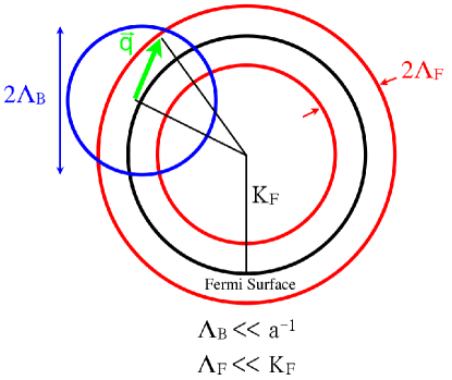
Figure 2: Kinematics of the RG rescaling ⁷⁰ for a system containing both gapless bosons, whose momenta are centered around a point in the momentum space, and gapless fermions, whose momenta are confined to the vicinity of a Fermi surface. $\Lambda_{B}$ and $\Lambda_{F}$ are the cut-off momenta for the bosons and fermions, respectively. $a$ is the lattice constant in real space.

4.1 The case of Fermi surface not intersecting the antiferromagnetic zone boundary

The analysis based on the combined fermion-boson RG has been discussed elsewhere ⁶⁸. The effective Kondo coupling, expressed in the QNL$\sigma$M representation by Eq. (57), is marginal at both the tree, one-loop, and infinite-loop levels. The tree level and one-loop analyses directly use the procedure of Ref. ⁷⁰, while the infinite-loop analysis was based on a decomposition of the Fermi surface into patches.

Here we present an alternative infinite-loop analysis without appealing to patching arguments. The goal of this analysis is to establish a type of Migdal’s Theorem which states that the tree-level result is the entire story. Since we found marginality at the tree-level, this is the exact answer to all orders in the limit where $\Lambda/K_{F}\to 0$.

For concreteness, we consider a spherical Fermi surface although generalizations to non-nested generic Fermi surfaces can be readily made. For a spherical Fermi surface we can write the Fermi momentum integral in terms of spherical coordinates:

$$\int d^{d}K = \int_{K_{F}-\Lambda}^{K_{F}+\Lambda}K^{d-1}dK\int d^{d-1}\Omega_{K}$$ (59)

$$= \int_{-\Lambda}^{\Lambda}(k+K_{F})^{d-1}dk\int d^{d-1}\Omega_{K}$$

The most relevant part of the above is

$$\int d^{d}K = K_{F}^{d-1}\int_{-\Lambda}^{\Lambda}dk\int d^{d-1}\Omega_{K}$$ (60)

Now the kinetic part of the fermions can be written,

$$\mathcal{S}_{c} = K_{F}^{d-1}\int dkd^{d-1}\Omega_{K}d\varepsilon\;\psi^{\dagger}(i\varepsilon-v_{F}k)\psi$$ (61)

We define new dimensionless variables:

$$\varepsilon = \Lambda\bar{\varepsilon}$$ (62)

$$k = \Lambda\bar{k}$$ (63)

$$\Omega_{K} = \bar{\Omega}_{K}$$ (64)

$$K_{F}^{d-1}\Lambda^{3}\psi^{\dagger}\psi = \bar{\psi}^{\dagger}\bar{\psi}$$ (65)

Note that the angular components of fermionic momenta are untouched. We now have:

$$\mathcal{S}_{c} = \int d\bar{k}d^{d-1}\bar{\Omega}_{K}d\bar{\varepsilon}\;\bar{\psi}^{\dagger}(i\bar{\varepsilon}-v_{F}\bar{k})\bar{\psi}$$ (66)

The important difference from the aforementioned patching argument is that now the fermionic fields contain factors of $K_{F}$. Plugging this into the Kondo coupling we find (note that the QNL$\sigma$M rescaling is identical to what was done in Ref. ⁶⁸)

$$\mathcal{S}_{K} = K_{F}^{1-d}\Lambda^{1+1+d+1-3+1-(d+3)/2}\lambda_{\perp}\int d\bar{k}d^{d-1}\bar{\Omega}_{K}d\bar{\varepsilon}d^{d}\bar{q}d\bar{\omega}[\bar{\psi}^{\dagger}\bar{\psi}(\bar{\omega}\bar{\pi})]$$ (67)

$$= \frac{\Lambda^{(d-1)/2}}{K_{F}^{d-1}}\lambda_{\perp}\int d\bar{k}d^{d-1}\bar{\Omega}_{K}d\bar{\varepsilon}d^{d}\bar{q}d\bar{\omega}[\bar{\psi}^{\dagger}\bar{\psi}(\bar{\omega}\bar{\pi})]$$ (68)

For $d=2$ we have

$$\frac{\mathcal{S}_{K}}{\mathcal{S}_{c}} \propto \frac{\sqrt{\Lambda}}{K_{F}}=\frac{1}{\sqrt{N_{\Lambda}}}\frac{1}{\sqrt{K_{F}}}$$ (69)

In the non-spin-flip channel:

$$\Gamma_{z} = K_{F}^{1-d}\Lambda^{1+1+d+1+d+1-3+1-2((d+3)/2)}\lambda_{z}\int d\bar{k}d^{d-1}\bar{\Omega}_{K}d\bar{\varepsilon}d^{d}\bar{q}_{1}d\bar{\omega}_{1}d^{d}\bar{q}_{2}d\bar{\omega}_{2}[\bar{\psi}^{\dagger}\bar{\psi}(\bar{\omega}\bar{\pi}\bar{\pi})]$$ (70)

$$= \frac{\Lambda^{d-1}}{K_{F}^{d-1}}\lambda_{z}\int d\bar{k}d^{d-1}\bar{\Omega}_{K}d\bar{\varepsilon}d^{d}\bar{q}_{1}d\bar{\omega}_{1}d^{d}\bar{q}_{2}d\bar{\omega}_{2}[\bar{\psi}^{\dagger}\bar{\psi}(\bar{\omega}\bar{\pi}\bar{\pi})]$$

For $d=2$,

$$\frac{\Gamma_{z}}{\mathcal{S}_{c}} \propto \frac{\Lambda}{K_{F}}=\frac{1}{N_{\Lambda}}$$ (71)

We have thus shown that for any $d>1$ the Kondo vertex will have associated with it positive powers of $1/N_{\Lambda}$. Because of this, as the number of powers of $J_{K}$ increases, so does the suppression factor $1/N_{\Lambda}$. The only exception is for a series of diagrams corresponding to a chain of particle-hole bubbles in the spin-flip channel ⁶⁸. Because the poles are located on the same side of the real axis, they make no contribution to the beta function ^{68, 50}. Thus, the tree-level result is the whole story, and the Kondo coupling is exactly marginal.

The RG result is further corroborated by a large-N calculation for the conduction electron Green’s function, which does not contain a pole and, correspondingly, the Fermi surface is small ⁶⁸.

4.2 The case of Fermi surface intersecting the antiferromagnetic Brillouin zone boundary

We now turn to the case where the Fermi surface intersects the AFBZ boundary. In this case, the linear coupling $\vec{n}\cdot\vec{s}_{c}$ between the local moments and conduction electron spin cannot be neglected. Until now, we have only considered the term $\vec{L}\cdot\vec{s}_{c}$ because our assumption has been that the Fermi surface does not intersect the AFBZ boundary, i.e. $Q>2K_{F}$. See Fig 1a and the comments following equation (49). When $Q<2K_{F}$, the conduction electrons see the AF order parameter of the local moments as a staggered scattering potential, resulting in a reconstruction of their Fermi surface. The hot spots of the Fermi surface therefore become gapped out, as shown in Fig. 1b. The effective coupling ⁶⁹ between the reconstructed quasiparticles and the $\vec{n}$ field involves a coherence factor containing an additional factor of $q$ (measured w.r.t. $\vec{Q}$). This linear-momentum suppression factor survives beyond the mean-field treatment of the conduction electron band, as dictated by Adler’s Theorem. Indeed, it can be viewed as a kinematic suppression similar to the deformation potential problem of the electron-phonon system ⁴⁴.

From the RG perspective, the additional factor of $q$ represents a decrease in the dimension of the coupling which has the same effect as a derivative coupling: $\vec{s}_{c}\cdot\vec{n}_{q}\to qa^{\dagger}\vec{\sigma}a\cdot\vec{n}_{q}$. Now the conduction electron spin is coupled directly to $\vec{n}_{q}$ which has dimension $\left[\pi_{q}\right]=-d-1$, but the additional factor of $q$ brings the dimension to $\left[q\;\vec{n}_{q}\right]=-d$ which has the same value as the vector field $\left[\vec{\varphi}_{q}\right]=-d$ we considered earlier for the case where the Fermi surface does not intersect the AFBZ boundary ⁶⁸. Therefore, our previous result on the marginality of the Kondo coupling is not spoiled when the Fermi surface intersects the magnetic zone boundary.

The marginal nature of the Kondo coupling implies that the effective Kondo coupling does not flow towards strong coupling. Correspondingly, there is no Kondo singlet formation in the ground state, and no Kondo resonances in the single-electron excitation spectrum. The absence of the Kondo resonance implies that the local moments remain charge-neutral, and the Fermi surface is determined by the conduction electrons alone; such a Fermi surface is called small, and the antiferromagnetic phase is named ${\rm AF_{S}}$. This is to be contrasted with what happens in an antiferromagnetic phase in the presence of Kondo resonances, in which the Fermi surfaces are specified by the hybridizing conduction electrons and the itinerant $f$-electrons that describe the Kondo resonances; such a Fermi surface is called large, and this antiferromagnetic phase is named ${\rm AF_{L}}$. Note that the presence of antiferromagnetic order can be incorporated in these definitions through an appropriate symmetry-breaking field  ³⁹.

5 Global phase diagram of the antiferromagnetic Kondo lattice

The establishment of the ${\rm AF_{S}}$ phase, along with the heavy-fermion ${\rm P_{L}}$ phase ^{5, 32}, provide two anchoring points in the heavy-fermion phase diagram at $T=0$. In order to connect these two phases, Ref. ⁵² introduced a two-parameter phase diagram, $(J_{K},G)$, which is shown in Fig. 3a. In units of conduction electron bandwidth, $J_{K}$ is the Kondo coupling while $G$ corresponds to magnetic frustration or reduced dimensionality. The latter is a measure of the quantum fluctuations amongst the local-moment degrees of freedom. It was also discussed in Ref. ⁵² that, for sufficiently large $G$, the conventional AF state of the local-moment component will yield to paramagnetic states which either preserve spin-rotational invariance (gapped or gapless spin liquid) or break it (spin Peierls). Inspired by the recent developments in doped ${\rm YbRh_{2}Si_{2}}$, this part of the phase diagram is explicitly included in the global phase diagram ⁵³ as shown in Fig. 3b. Related considerations on the global phase diagram are also being made in Ref. ⁹.

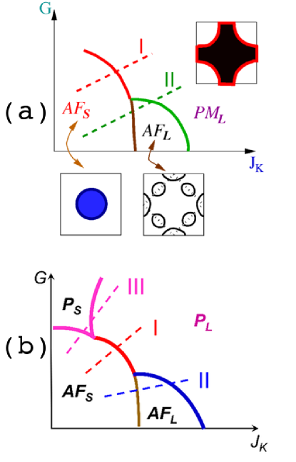
Figure 3: (a) Global phase diagram with the illustrative Fermi surfaces. (From ⁵².) (b) Global phase diagram showing the three different types of trajectories for quantum phase transitions. This phase diagram has a remarkable correspondence with what happens in heavy fermion metals. (From ⁵³.)

This global phase diagram can be described in terms of three possible trajectories that connect the ${\rm AF_{S}}$ phase and ${\rm P_{L}}$ phase, as specified in Fig. 3b. Trajectory $I$ goes directly between the ${\rm AF_{S}}$ and ${\rm P_{L}}$ phases, giving rise to a local quantum critical point: the collapse of Kondo resonances occurs at the magnetic quantum critical point – in the notation of Refs. ^{54, 55, 57}, $\delta_{c}$ and $\delta_{loc}^{c}$ are located at the same place. As the Kondo effect is continuously broken down at the AF QCP, there is a sudden jump between the large Fermi surface and the small one  ^{54, 10, 55, 57}, and the Kondo-breakdown scale $E_{\mathrm{loc}}^{*}$ vanishes at the QCP. Correspondingly, the residues associated with both the small and large Fermi surfaces vanish as the QCP is approached from either side ^{54, 10, 55, 52, 48}. Our considerations of the global phase diagram puts local quantum criticality in a larger perspective.

Along Trajectory $II$, the transition between the ${\rm AF_{S}}$ and ${\rm P_{L}}$ phases involve an intermediate ${\rm AF_{L}}$ phase. This is the SDW state of the heavy quasiparticles of the ${\rm P_{L}}$ phase. The magnetic-to-paramagnetic transition is of the SDW type ^{25, 31, 33}. A Kondo breakdown transition can still take place at the ${\rm AF_{L}}-{\rm AF_{S}}$ boundary ^{52, 68}; in typical cases, this corresponds to a a Lifshitz transition with a change of Fermi surface topology.

Finally, along Trajectory $III$, the transition goes through the intermediate ${\rm P_{S}}$ phase. This is a paramagnetic phase with a small Fermi surface. The small-to-large Fermi surface transition could be either a spin-liquid ^{49, 3} to heavy-Fermi-liquid QCP, or a spin-Peierls to heavy-Fermi-liquid QCP ³⁹.

There is overwhelming evidence that pure ${\rm YbRh_{2}Si_{2}}$ at ambient pressure displays a type-I quantum phase transition. Recently, Friedemann et al. ¹⁸ showed that enough Co-doping (of nominally 3% or more), which introduces positive chemical pressure, turns the transition into one whose properties are largely compatible with the type-II transition. Preliminary studies have shown that a similar effect arises in pure ${\rm YbRh_{2}Si_{2}}$ under a sufficiently large pressure ⁶⁵. A relatively small amount of (nominally 2.5%) Ir-doping, which introduces negative chemical pressure, retains the type-I transition ¹⁸. By contrast, a larger negative chemical pressure, corresponding to a larger amount (nominally 6% or more) Ir- doping, turns the transition into one that is compatible with a type-III transition. A similar behavior has also been seen in Ge-doped ${\rm YbRh_{2}Si_{2}}$ ¹². Experimentally, there is an indication that the regime corresponding to $P_{S}$ has non-Fermi liquid behavior, raising the exciting possibility that this is in fact a non-Fermi liquid phase.

6 Kondo insulators

Heavy fermion metals involve localized magnetic moments and a partially-filled conduction-electron band. This can be generically modeled in terms of a Kondo lattice Hamiltonian comprising two specifies of electrons: a lattice of spin-$1/2$ local moment, with one per unit cell; and a band of conduction electrons with a filling of $0<x<1$ electrons per unit cell.

When $x=1$, we have an even number of electrons per unit cell and an insulator becomes a natural possibility. In fact, the analogue of the ${\rm P_{L}}$ phase of the $0<x<1$ case is the Kondo insulator². For $x=1$, the Kondo-singlet formation in the ground state induces delocalized $f$-electron quasiparticles, which hybridizes with the conduction electron band and induces a hybridization gap at the Fermi energy. At zero-field, it is traditionally believed that the Kondo insulator is the only possible phase. (By contrast, a large magnetic field can suppress the Kondo effect altogether, inducing a magnetically ordered metal ².)

Here, we make the observation that the ${\rm AF_{S}}$ phase extensively described above remains a stable phase for the $1+1$ “Kondo-insulator filling.” The exchange interaction between the local moments in this regime is generically expected to be antiferromagnetic. In addition, in the parameter regime specified by Eq. (7), our asymptotically exact RG analysis of the Kondo lattice Hamiltonian in its QNL$\sigma$M representation continues to apply, regardless of whether the underlying conduction electron Fermi surface intersects the AFBZ boundary. To the same degree of confidence as in the case of generic filling, the small-Fermi-surface paramagnetic ($P_{S}$) phase is also expected to occur in the case of $1+1$ filling when the the parameter $G$ (the quantum fluctuations of the local-moment component) becomes sufficiently large and for small Kondo coupling.

The above assumes that there is no perfect nesting of the conduction electron Fermi surface. A perfect nesting with $x=1$ would only occur for a square lattice with strictly no hopping beyond nearest neighbors, and this is unlikely to be the case for rare-earth intermetallics.

These considerations lead to a global phase diagram for Kondo insulators, shown in Fig. 4. The list of materials believed to be Kondo insulators is by now relatively large. It will be instructive to search for quantum phase transitions out of a Kondo insulator and into either the ${\rm AF_{S}}$ or ${\rm P_{S}}$ metallic phases. While it is in general hard to predict precisely which trajectory a particular tuning parameter – such as pressure or chemical doping – would correspond to in such a global phase diagram, what is minimally required is to increase the ratio of the AF RKKY interaction to the Kondo coupling. For Ce-based systems, this happens with the application of a negative (chemical) pressure. For Yb-based systems, on the other hand, this is achieved by applying a positive (chemical) pressure.

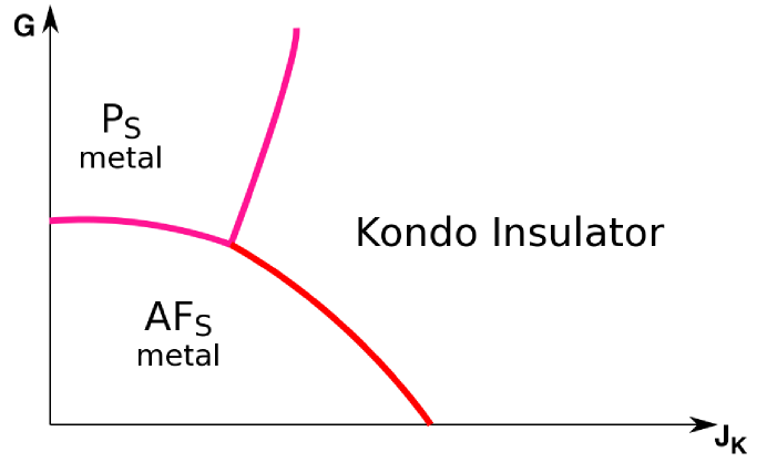
Figure 4: Global phase diagram for Kondo-insulator systems. The Kondo-insulator phase corresponds to a Kondo-singlet ground state, and is paramagnetic. ${\rm AF_{S}}$ describes an antiferromagnetic metal state with a small Fermi surface and ${\rm P_{S}}$ a paramagnetic metal phase also with a small Fermi surface; each has the same meaning as its counterpart in Fig. 3.

7 Connection to the holographic theory of non-Fermi liquid

There has been considerable recent interest in applying the techniques developed in string theory to many-body systems. These developments rely on a duality between a $d$-dimensional strongly-coupled field theory and a quantum-gravity theory in a weakly curved $(d+1)$ dimensional anti-de Sitter (AdS_d+1) spacetime. Non-Fermi liquid behavior has been studied through a charged black hole in the AdS spacetime ^{28, 29, 11, 15, 40}. In this approach, the fermionic self energy shows a marginal-Fermi-liquid-like form ⁶⁶. This has been clarified as originating from an infrared fixed point characterized by a $(0+1)$-dimensional conformal field theory ¹⁵, which is dual to a near horizon geometry AdS${}_{2}\times\mathbb{{R}}^{d-1}$. The $(0+1)$-dimensional conformal field theory corresponds to a quantum impurity model.

The factorization of temporal and spatial correlations become more transparent in a “semi-holographic” formulation ^{16, 15}, in which a conduction-electron band is introduced to be hybridized with the fermions in a strongly coupled field theory dual to the gravity theory. In turn, this allows an Anderson-lattice-model interpretation (see also Ref. ⁴¹), in which the fermions of the strongly coupled field theory is the analogue of the $f$-electron degree of freedom of the Anderson lattice model. The relevance or irrelevance of the hybridization may then be linked to the Kondo screening or Kondo breakdown of a class of quantum impurity models – the Bose-Fermi Kondo model – coupled to a fermionic bath ^{59, 47, 74, 71}. In the Kondo language, a breakdown of the Kondo effect, occurring when the hybridization-induced Kondo coupling is irrelevant or marginal in the RG sense, leads to a power-law form of the conduction-electron self-energy whose exponent is positive; such a form of the self-energy appears in the non-Fermi liquid state of the holographic models ^{28, 29, 11, 15, 40}. A Kondo-screened state, occurring when the hybridization-induced Kondo coupling is relevant in the RG sense, gives rise to a pole in the conduction-electron self-energy. No such a form of the self-energy has been identified so far in the holographic models.

These considerations point to a linkage between the Kondo-breakdown physics of the Kondo/Anderson lattice systems and the fate of the non-Fermi liquid state dual to the gravity theory with a near-horizon AdS${}_{2}\times\mathbb{{R}}^{d-1}$ geometry. There could be at least two possibilities for the latter. One possibility is that the non-Fermi liquid state is unstable towards an antiferromagnetically-ordered state with a small Fermi surface discussed earlier, but retains a similar form in the quantum-critical regime; this is the analogue of the Kondo-breakdown physics in the local quantum criticality formulation ^{54, 55}. Note that the entropy vanishes at the local quantum critical point ¹³. An alternative is that this state is unstable towards a paramagnetic phase with a small Fermi surface ⁴¹, as occurring in one formulation of the Kondo breakdown ^{49, 38}. In either case, these considerations suggest that holographic models may contain an analogue of the paramagnetic phase with a large Fermi surface, whose conduction-electron self-energy singularly depends on energy (containing a pole) and smoothly depends on momentum.

With these considerations in mind, it will be instructive to study itinerant magnetic systems from the gravity side. A recent work has gone along this direction ²⁶.

8 Conclusions

Recent theoretical and experimental developments have opened up the issue of the global phase diagram in heavy fermion metals. We discussed some of the earlier developments that have led to the continued theoretical efforts on the global phase diagram, and the striking recent experiments that point to the richness of the quantum phase transitions between antiferromagnetic and paramagnetic heavy fermion metals.

We provided the details of the asymptotically exact analysis of the Kondo lattice in the antiferromagnetic part of the phase diagram. General considerations on the transitions from the Kondo-breakdown antiferromagnetic metal phase with a small Fermi surface to the Kondo-screened paramagnetic heavy fermion phase have motivated a global phase diagram, which is consistent with earlier studies of the Kondo breakdown effect from the paramagnetic side including the distinction between the local quantum critical point and the SDW quantum critical point. Our considerations also put earlier formulations of the Kondo breakdown effect in the paramagnetic region into a general perspective. Model studies that can cover all these different phases and transitions in one unified framework are called for.

We have also discussed the Kondo insulators along a similar line. We have proposed a related global phase diagram for such systems, which we hope will stimulate future experiments.

Finally, we have discussed the connection between the Kondo-breakdown local quantum criticality of Kondo lattice systems and the holographic non-Fermi liquid behavior. Considerations of magnetic states and quantum magnetic transitions from a gravity dual are just beginning. Conversely, studies of quantum critical behavior in magnetic many-body systems, including heavy-fermion metals and insulators, may shed some light on gravity problems.