Reply to Comment on “Electron transport through correlated molecules computed using the time-independent Wigner function: Two critical tests”

Abstract

In their Comment, Greer et al (i) put us in charge of a pretended wrong claim, which we never made in Phys. Rev. B 78, 115315 (2008), where we criticized a method (DG) proposed by two of them, (ii) incorrectly claim that the DG method can reproduce the conductance quantum $g_{0}$, but (iii) to deduce $g_{0}$ for a toy model, they carry out calculations within the standard Landauer method, which has nothing to do with the DG’s. We present results for their model obtained within the DG method, which demonstrate that the DG method fails as lamentably as in the examples we presented in our earlier work. We also analyze the physical reasons why the DG method fails.

I Introduction

In their Comment,GreerComment:09 Greer, Delaney, and Fagas (henceforth GDF) claim that they can resolve the conundrum expressed in our paper Baldea:2008b (referred to as I below), where we challenged a method (DG) put forward by two of them in Ref. DelaneyGreer:04a, and subsequently used in their Refs. DelaneyGreer:04b, ; DelaneyGreer:06, ; Fagas:07, . Unfortunately, their attempt to refute our criticism of I (a reference which GDF even omit in their bibliography list) is based on a series of inaccuracies and statements without any support. This starts from the abstract of Ref. GreerComment:09, , wherein GDF incorrectly state that we criticized a so-called MECS (many-electron correlated scattering) approach, which was not even mentioned in I, nor defined in the works DelaneyGreer:04a, ; DelaneyGreer:04b, ; DelaneyGreer:06, ; Fagas:07, that made the object of our criticism. Before discussing the controversial issues in detail, we emphasize the following:

(i) Using the acronym MECS, GDF obviously distract attention from the fact that the (DG) method DelaneyGreer:04a ; DelaneyGreer:04b ; DelaneyGreer:06 ; Fagas:07 envisaged by us is manifestly a variational one. In their “brief introduction to the MECS approach” (Sect. II of Ref. GreerComment:09, ), they completely omit to state that the variational ansatz (namely, the minimization of the total energy in the presence of an external bias $V$) is an essential ingredient of the DG method; in that introduction, they do not define a transport approach, but merely review well known properties of the Wigner function (WF) $f(q,p)$.

(ii) With this acronym and “carefully” chosen quotations from I, by only mentioning in passing “the variational structure of the MECS calculations performed to date …” (Sect. V), without noting that all their calculations criticized in I are variational, they aim to convey the false impression that the DG method merely consists of open boundary conditions (OBCs) expressed in terms of the WF, and that I only criticizes these WF-OBCs. We stress from the very beginning that what we criticized in I is the DG variational approach as such, and in particular the WF-OBCs in the specific context of that method employed to a finite cluster; the DG approach, as any transport theory, cannot be reduced to whatever boundary conditions (BCs).

(iii) None of the results of GDF (their Sect. IV) were obtained within the DG method, but simply within the well-established Landauer approach for an uncorrelated toy model (GDF model hereafter).toy

GDF mainly claim that: our critique in I of the DG method is invalid, and they present calculations within a simple model that reproduce the conductance quantum $g_{0}$. The first claim is wrong, as explained in Sect. II. In Sect. III, we show that the second claim is irrelevant, because their derivation of $g_{0}$ is done within the Landauer approach and not within the variational DG approach criticized by us. Some challenges to the results thus obtained by GDF are presented in Sect. IV. Next, in Sect. V we present results for the GDF model deduced within the DG method, which clearly demonstrate the failure of that method. The other issues raised by GDF are addressed in Sect. VI. In Sect. VII we indicate the physical reasons why the DG method fails. Conclusions are presented in Sect. VIII.

II Refuting the GDF criticism to our work

The main presumptions made by GDF to refute the criticism of I are that: (i) we incorrectly presumed an asymmetric injection of momentum, (ii) we incorrectly assumed that there is no chemical potential difference when applying OBCs, and (iii) we appear to be confusing in the application of OBCs when using either momentum or energy distributions.

All these claims are wrong. To arrive at our basic Eqs. (19-21), which yielded the results presented in Figs. 2—5, and 7, demonstrating the lamentable failure of the DG method, we made exactly what that method prescribes: energy minimization, Eq. (1), with WF-OBCs, Eqs. (5, 6), wave function normalization, Eq. (9), and, if not otherwise specified, current conservation, Eq. (8). More specifically:

To (i): A momentum asymmetry was assumed neither in the analytical results of Eqs. (19-21), nor in the numerical results of Figs. 2—5, and 7. In our WF-OBCs, Eqs. (5, 6), the “momenta” $p_{L,R}$ in the LHS and RHS are the same. Otherwise, we should have written, e.g., $f(q_{L,R},p_{L,R}\pm\delta p)=f_{0}(q_{L,R},p_{L,R})$, $\delta p=\mathcal{O}(V)$.

To (ii): This is wrong, we do assume a nonvanishing chemical potential difference ($eV$). The bias $V$ enters our calculations, because the quantity to be minimized of Eq. (1) does depend on it via $W$. Consequently, the wave function $\Psi$ obtained within the DG procedure does contain an asymmetry between the left and right electrodes for $V\neq 0$, and this asymmetry reflects itself in the WF at the boundaries. Without this dependence, e. g., the quantity $\delta f=f-f_{0}\neq 0$ for electrons flowing from the device into electrodes displayed in Fig. 2 would have been zero.

To (iii): By faithfully applying the DG method to well-defined models in I, we were simply faced with a mathematical problem whose solution is exact and unique within the linear response theory, and unambiguously yields unphysical results. We needed not explicitly discuss, e. g., the distinction between momentum and energy distributions.

The numerical results presented in I, which are completely unphysical, are nothing but the results of the variational DG method, because in I we did nothing else than exactly what that method prescribes. Therefore, any critique to I represents in reality a critique of the DG method itself.

III Rebuttal of the claim on the reproduction of the conductance quantum

GDF write: “In practice, the” WF “is used to constrain the momenta flow out of the electron reservoirs and into the scattering region” (Sect. II). This “practice” does not obviously refer to the Comment; simply, GDF use Eqs. (3–5) nowhere in calculations (not even in their envisaged works). Relevant for the present debate would have been to apply the variational DG approach (including its original WF-OBCs) and see whether it is able to correctly describe the transport, and not to show that another (Landauer’s) approach can reproduce correct results (conductance or WF).

In the Comment, GDF do nothing else than apply the standard Landauer approach to deduce the conductance [see their Eqs. (12) and (13)] and to compute the WF in electrodes’ middle. So, they cannot pretend that the variational DG approach correctly reproduces the conductance of their simple uncorrelated model. Their statement in Introduction that in “Sect. IV a calculation of conductance quantization …is given using the MECS construction” is not true. Equally wrong is their claim that the BCs “as formulated in MECS applied to” their “model reproduces the well-known result of conductance quantization”. We did not challenge the Landauer approach, and the fact that using it GDF can deduce a correct result ($g_{0}=e^{2}/h$) for an uncorrelated model, which is trivial from the point of view of the Landauer approach, is not at all astonishing: the transmission through a barrier of vanishing height ($V\to 0$) is equal to unity. This correct result, deduced within a correct approach, has absolutely no relevance for the validity of the variational DG method, and our critique of the latter is not in the least affected. In the GDF calculations, BCs are imposed not by using the WF but by simply postulating standard scattering forms of the asymptotic single-electron wave functions [Eqs. (7) and (11)]. They use these forms, in a kind of a posteriori check, to show that the WFs computed within the Landauer approach, in and out of equilibrium, at carefully chosen boundaries behaves as expected physically. Computing the WF within the Landauer approach (and not within the DG’s) and claiming that “indeed it is observed that in the single particle case constraining the incoming momentum inflow via the Wigner function implies solving the Schrödinger equation …” (Sect. IV.A of GDF) is totally unfounded. The GDF calculation represents in itself a logical inconsistency hard to understand: within Landauer calculations, they assume Fermi distributions (shifted in energy by $\mu_{R}-\mu_{L}=eV$ for $V\neq 0$) in electrodes, and show that the WFs (approximately) just look like the Fermi functions already postulated. Within this philosophy, one can solely infer that the Landauer approach is indeed self consistent, but this is trivial and irrelevant for the validity of the DG’s.

As noted in Introduction, GDF wish to reduce the whole debate to the WF-OBCs, but no transport theory can be solely reduced to a certain type of BCs. In I we criticized the WF-OBCs in the specific context of the variational DG method, and did not challenge the WF-OBCs in general. See the end of the third paragraph on page 2 of I and the lines after Eqs. (3) and (4) in I], or what we explicitly wrote (last paragraph of I): “While the idea of formulating boundary conditions in terms of the Wigner function for correlated many-body systems is interesting, the manner in which it was imposed in” Ref. DelaneyGreer:04a, “turns out to be inappropriate.”

By deducing a simple result within the Landauer approach and not within the DG’s, GDF raise very serious doubts that they can also derive the correct result within the latter. Confirming these doubts, we shall demonstrate in Sect. V that for the simple model of their choice, the DG approach fails as lamentably as in the cases presented in I.

IV Challenges to the GDF calculations

The GDF’s Landauer calculations affect in no way our critique to the DG method. However, especially because GDF attempt to present these results as if they were related to Ref. DelaneyGreer:04a, , we note several errors of Ref. GreerComment:09, .

For the GDF model, the transmission can be trivially obtained analytically, $T(\varepsilon)=4k_{L}k_{R}/(k_{L}+k_{R})^{2}$, $k_{L}\equiv\sqrt{2m\varepsilon}/\hbar$, and $k_{R}\equiv\sqrt{2m(\varepsilon-eV)}/\hbar$, Constantinescu and it yields the following exact expression of the current

$$\displaystyle I(V) = -\frac{e}{h}\frac{8\varepsilon_{F}}{n_{F}^{2}}\sum_{n_{L}\geq n_{V}}^{n_{F}}\frac{n_{L}^{2}x_{R}}{\left(n_{L}+x_{R}\right)^{2}}+\frac{e}{h}\frac{8\varepsilon_{F}}{n_{F}^{2}}\sum_{n_{R}=1}^{n_{F}}\frac{x_{L}n_{R}^{2}}{\left(x_{L}+n_{R}\right)^{2}}\stackrel{{\scriptstyle L\to\infty}}{{\longrightarrow}}Vg_{L}(eV/\varepsilon_{F}),$$

$$g_{L}(x) \equiv g_{0}\frac{8}{3x^{3}}\left[\frac{x^{3}}{2}+\sqrt{1+x}-\sqrt{1-x}+x\left(\sqrt{1+x}+\sqrt{1-x}-3\right)\right];\lim_{x\to 0}g_{L}(x)=g_{0},$$ (1)

$$x_{L,R} \equiv \sqrt{n_{R,L}^{2}\pm n_{V}^{2}},n_{V}\equiv n_{F}\sqrt{eV/\varepsilon_{F}}.$$

The above $n_{V}$ coincides with the RHS of GDF’s Eq. (16).

Instead of giving these simple formulas, GDF present some qualitative considerations aiming to show that (i) the conductance quantum is correctly reproduced, and (ii) this result has something to do with the results and the electrode sizes ($L\approx 2$ nm) of their controversial works.DelaneyGreer:04a ; DelaneyGreer:04b ; DelaneyGreer:06 ; Fagas:07 To deduce $g_{0}$ in Sect. IV.B, they approximate $T(\varepsilon)\simeq T(\varepsilon_{F})\simeq 1$; this amounts to implicitly assume the linear response limit ($eV\ll\varepsilon_{F}$). In the last paragraph of Sect. IV.A, GDF claim that their considerations to deduce $g_{0}$ “apply well to electrode lengths as small as $1$ nm”($=L/2$). They assume that $n_{F}$ is large and $\Delta k=2\pi/L$ is small [this should mean that $n_{F}=k_{F}L/2\pi\gg 1$ and $\Delta k=2\pi/L\ll k_{F}$, cf. Eq. (7) of GDF]. For $L=2$ nm and their completely unphysical value $k_{F}=0.12$ nm^-1 (cf. Fig. 3 of Ref. GreerComment:09, ), one gets $n_{F}=0.0038$ (!) and $\Delta k=3.14$ nm${}^{-1}\gg k_{F}$(!). In reality, to mimic gold electrodes (Fermi velocity $v_{F}\simeq 1.4\times 10^{6}$ m/s, $\varepsilon_{F}=mv_{F}^{2}/2\simeq 5.6$ eV), one needs a $k_{F}$-value hundred times larger, $k_{F}\simeq 12$ nm^-1. Even then, one gets $n_{F}=3.8$, and satisfying the above conditions is problematic. In fact, to derive Eq. (18) from Eq. (17) in Ref. GreerComment:09, GDF need not a large $n_{F}$, but rather a large $n_{V}$, which should obviously be much smaller than $n_{F}$. If we admit that $n_{V}=2$ is a number “much” larger than unity and “much” smaller than the other “large” number $n_{F}\lesssim 4$, Eq. (1) leads to $V\sim 1$ volt.

How poor is the linear approximation in this range and how bad is the description based of electrodes with $L=2$ nm, exactly the linear sizes of the $Au_{13}$ and $Au_{20}$ clusters used in GDF’s ab initio works,DelaneyGreer:04a ; DelaneyGreer:04b ; DelaneyGreer:06 ; Fagas:07 can be seen in Fig. 1, and any further comments are superfluous. If, as in the present case, the exact current for $L\to\infty$ is known, one may still argue that the “correct” trend can be unraveled by a “clever” inspection of the curve for very short electrodes ($L=2$ nm) in Fig. 1. However, one may more legitimately ask how reliable could be considered a theoretical result obtained with very short electrodes in implementations for complex realistic cases (like those of Refs. DelaneyGreer:04a, ; DelaneyGreer:04b, ; DelaneyGreer:06, ; Fagas:07, ) where neither the exact values nor the electron spectrum details are known a priori. From the curve for $L=2$ nm of Fig. 1 one deduces a linear conductance ($V\to 0$) of $\sim 10^{-2}g_{0}$, i. e., hundred times smaller than the true value $g_{0}$.

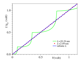
Figure 1: I-V characteristics obtained exactly from Eq. (1) for infinite electrodes with $k_{F}=12$ nm^-1 (as in gold), and for two finite sizes $L$ (given in the legend).

As their results on the WFs obtained within the Landauer approach are irrelevant for the DG validity, we restrict ourselves here to a few critical remarks. In Sect. II, GDF mention that the WF, as a function of energy defined in the phase space, tends rapidly toward the Fermi distribution with increasing number $N$ of particles in a confining potential. Indeed, in their Ref. 9, Cancellari et al showed that $\mathcal{F}(\varepsilon_{p})\sim\int_{\varepsilon_{p},\varepsilon_{p}+\delta\varepsilon_{p}}d\,\mathbf{q}_{1}^{N}d\,\mathbf{p}_{1}^{N}f^{(N)}(\mathbf{q}_{1}^{N},\mathbf{p}_{1}^{N})$ behaves as the Fermi distribution $f(\varepsilon_{p})$. Notice that the system of that Ref. 9 is confined (while GDF use periodic BCs, $k_{n}=2\pi n/L$), and Cancellari et al attribute a physical meaning to a function whose argument is the energy $\varepsilon_{p}$, which is unequivocally defined in the uncorrelated case discussed by GDF, and not to a function of momentum $p$. Contrary to them, GDF ascribe a physical meaning to $f(q_{L,R},p)$, i. e., at fixed locations (without $q$-integration) and interpret $p$ as a physical momentum of electrons, e. g., which move toward right for $p>0$ and toward left for $p<0$. We do not analyze here $f(q,p)$ at $V\neq 0$.Baldea:unpublished We only point out an error in the Comment for $V=0$. The exact expression of their Eq. (10) deduced from their formulas for finite $L$ is

$$\displaystyle f_{0}(-\frac{L}{4},p) = \frac{2}{L}\sum_{n=1}^{n_{F}}\left\{\frac{\sin\left[\left(p/\hbar+k_{n}\right)L/2\right]}{p/\hbar+k_{n}}+\frac{\sin\left[\left(p/\hbar-k_{n}\right)L/2\right]}{p/\hbar-k_{n}}\right\}$$ (2)

$$= \frac{\sin\pi P}{\pi}\sum_{n=1}^{n_{F}}(-1)^{n}\left(\frac{1}{P+n}+\frac{1}{P-n}\right),$$

where $P\equiv n_{F}p/(\hbar k_{F})$. Inspecting Eq. (2), one can immediately see that the RHS vanishes for $p=0$. Therefore, their formula and the curves for $L=2$ nm and $L=20$ nm of their Figs. 3a and b are incompatible (the case $q_{R}=+L/4$ is similar). The Wigner function computed by means of Eq. (2), i. e., GDF’s own formula for their sizes is shown in Fig. 2a.round-L As visible there, the dip around $p=0$ [of a width $\delta p=2\hbar k_{F}/n_{F}\propto 1/L$, cf. Eq. (2)], becomes narrow only at larger $L$. If GDF used their formula to compute the WF at $q_{L,R}=\mp L/4$, they would have shown the curve of our Fig. 2a, not too much resembling a Fermi distribution for $L=2$ nm, which mimics their gold electrodes.DelaneyGreer:04a

       

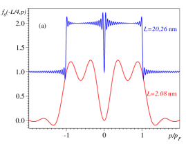
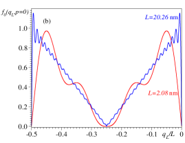
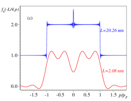
Figure 2: Equilibrium Wigner function computed: (a, b) using the GDF formulas, and (c) for a confined system for two sizes $L$ (given in the legend) and $k_{F}=p_{F}/\hbar=12$ nm^-1.

Limitations of the physical meaning of the WF are well known.mahan ; frensley:90 ; Datta:97 Noteworthy, in emphasizing these limitations even at equilibrium, textbooks (see, e. g., Ref. mahan, , ch. 3.7, pp. 202-203) choose typical examples just like the one invoked by GDF (cf. Sect. IV.A) to claim that the WF is physically useful. The fact that the boundary locations whereat the WF was computed by GDF cannot be arbitrary and should be “carefully” chosen (just in electrodes’ middle to GDF, $q_{L,R}=\mp L/4$) already raises warning bells on its appropriateness for applying BCs. Generalizing Eq. (2) away from $q_{L,R}=\mp L/4$ by restricting the integration $r$-range to either electrode in the GDF formulas is straightforward. To illustrate the sensitivity of $f_{0}(q_{L},p)$ to the boundary location, we depict in Fig. 2b the component $p=0$, a classical textbook’s example (e. g, ch. 8.8, p. 327 of Ref. Datta:97, ), which defies a simple physical interpretation. Noteworthy, our results of the genuine DG calculations in I are quite unphysical even with this choice (boundaries exactly in electrodes’ middle): this is just the choice in Fig. 7, this choice also qualitatively changes nothing in Fig. 3.

V Results of the variational DG method for the GDF model

We proceed by showing what GDF should have shown, namely the results of the variational DG method for the chosen model. To obtain the linear response of the GDF model, the working equations (5-21) of I (which yield an exact and unique solution) deduced from the faithful implementation of the variational DG method without any other extra assumption (cf. Sect. II), can be straightforwardly used. Only a minor adaptation is needed in Eqs. (7), (10), and (12), namely to consider a continuous space coordinate $-L/2<x<L/2$ instead of a discrete lattice, and this will be briefly indicated below. An important strong point of the approach of I is that it allows to determine self-consistently the limit of its applicability, namely the highest bias $V<V_{lr}$ compatible with the linear response approximation. For this, the expansion coefficients $A_{n}=\mathcal{O}(V)$ [$\Psi=A_{0}\Psi_{0}+\sum_{n\neq 0}A_{n}\Psi_{n}$, $A_{0}=1-\mathcal{O}(V^{2})$] should satisfy the condition $\mathcal{S}\equiv\sum_{n}|A_{n}|^{2}\ll 1$. As a practical numerical criterion we imposed $\mathcal{S}=0.01$, which typically yielded $V_{rl}\sim 1$ volt. Therefore, all numerical results presented in this section for $V\neq 0$ are for $V=1$ volt.

Without applied bias ($V=0$), an eigenstate $k$ of each electron out of the $N$ noninteracting electrons considered is characterized by a wave function $\phi_{k}(x)$ and an energy $\varepsilon_{k}$ satisfying the Schrödinger equation

$$h(x)\phi_{k}(x)\equiv\left[-\frac{\hbar^{2}}{2m}\frac{d^{2}}{d\,x^{2}}+v(x)\right]\phi_{k}(x)=\varepsilon_{k}\phi_{k}(x).$$ (3)

The second quantized electric current $\hat{j}(x)$ and Fano $\hat{F}(q,p)$ operators needed to compute the linear response read

$$\hat{j}(x)=\sum_{k,k^{\prime}}J_{k,k^{\prime}}(x)c_{k}^{\dagger}c_{k^{\prime}};J_{k,k^{\prime}}(x)=i\frac{e\hbar}{2m}\left[\phi_{k}^{\ast}(x)\frac{\partial\phi_{k^{\prime}}(x)}{\partial x}-\frac{\partial\phi_{k}^{\ast}(x)}{\partial x}\phi_{k^{\prime}}(x)\right];$$ (4)

$$\hat{F}(q,p)=\sum_{k,k^{\prime}}F_{k,k^{\prime}}(q,p)c_{k}^{\dagger}c_{k^{\prime}};F_{k,k^{\prime}}(q,p)=\int d\,r\phi_{k}^{\ast}(q-r/2)\phi_{k^{\prime}}(q+r/2)e^{-ipr/\hbar}.$$ (5)

The action of an applied voltage $V(x)$ is expressed by

$$\hat{W}=\sum_{k,k^{\prime}}V_{k,k^{\prime}}c_{k}^{\dagger}c_{k^{\prime}};V_{k,k^{\prime}}=-e\int_{-L/2}^{L/2}d\,x\phi_{k}^{\ast}(x)\phi_{k^{\prime}}(x)V(x).$$ (6)

For the GDF potential, the antisymmetric form $V(x)=V/2$ if $-L/2<x<0$, and $V(x)=-V/2$ if $0<x<L/2$ is more convenient, because it permits to separate the even ($\Psi_{g}$) and odd ($\Psi_{u}$) many-body eigenstates, as discussed in I. For this, it is necessary to further assume a symmetric potential barrier $v(-x)=v(x)$, which can be also included to make the calculations a bit more realistic. This (let us call it statical) barrier should not be confused with the barrier $V(x)$ related to the applied bias. For the GDF model, $v(x)\equiv 0$, and $\varepsilon_{k}=\hbar^{2}k^{2}/(2m)$. Within the DG approach, the system is confined within $-L/2<x<L/2$, $\phi_{k}(\pm L/2)\equiv 0$, and therefore $\phi_{k_{n}}^{g}(x)=\sqrt{2/L}\cos(k_{n}x)$ and $\phi_{k_{n}}^{u}(x)=\sqrt{2/L}\sin(k_{n}x)$, where $k_{n}\equiv\pi n/L$. For even eigenstates (superscript $g$), $n=1,3,5,\ldots$ is odd, while for odd eigenstates (superscript $u$), $n=2,4,6,\ldots$ is even. In the ground state $\Psi_{0}$, the highest occupied single electron level has $k=k_{F}=\pi N/L$. GDF’s electron orbitals $\phi_{k_{n}}(x)=\exp(ik_{n}x)/\sqrt{L}$ satisfy periodic BCs, $k_{n}=2\pi n/L$, where $n$ is a signed integer ($-n_{F}\leq n\leq n_{F}$). Without asking whether it makes sense to consider systems which are not confined within the original variational DG approach, for completeness and for comparison with the exact results for the GDF model (Sect. IV), we carried out calculations for both cases (termed confined and periodic below).

Because the operators $\hat{W}$, $\hat{j}$, and $\hat{F}(q,p)$ are bilinear, all their matrix elements $\langle\Psi_{n}|\ldots c_{k}^{\dagger}c_{k^{\prime}}|\Psi_{0}\rangle$ needed as input into the working Eqs. (12)—(21) of I can be obtained exactly. All the exact excited many-electron eigenstates $\Psi_{n}$ that contribute are particle-hole excitations, $|\Psi_{n}\rangle\to|\Psi_{k,k^{\prime}}\rangle=(-1)^{S_{k,k^{\prime}}}c_{k}^{\dagger}c_{k^{\prime}}|\Psi_{0}\rangle$. Here, the sign factor accounts for the ordering adopted to fill the Fermi sea. So, exactly as in I, we can present exact full CI calculations done within the DG approach, and the results should be exact if that approach were valid.

Within its variational scheme, the DG approach determines the steady state $\Psi$ at $V\neq 0$ by constraining the WF of incoming electrons at the electrode-device boundaries (at $q_{L,R}=\mp L/4$, as by GDF) to that of the ground state $\Psi_{0}$

$$f(q_{L,R},\pm p>0)\equiv\langle\Psi|\hat{F}(q_{L,R},\pm p>0)|\Psi\rangle=\langle\Psi_{0}|\hat{F}(q_{L,R},\pm p>0)|\Psi_{0}\rangle\equiv f_{0}(q_{L,R},\pm p>0).$$ (7)

The constrained minimization of the total energy allows the system ($-L/2<x<L/2$) to optimize the WF of outgoing electrons and therefore the differences below are allowed to be nonvanishing

$$\delta f(q_{L,R},\mp p>0)\equiv f(q_{L,R},\mp p>0)-f_{0}(q_{L},\mp p>0)=\langle\Psi|\hat{F}(q_{L,R},\mp p>0)|\Psi\rangle-\langle\Psi_{0}|\hat{F}(q_{L,R},\mp p>0)|\Psi_{0}\rangle\neq 0.$$ (8)

Due to this fact, by mathematical construction, the DG steady state breaks the time reversal. In Fig. 2c, we present results for the WF $f_{0}(q_{L},p)=f_{0}(q_{R},p)$ in the ground state $\Psi_{0}$ of the confined system. Comparing panels $a$ and $c$ of Fig. 2 one can see that, as expected for any physically relevant quantity, the equilibrium WF saturates at sufficiently large sizes $L$ and becomes independent on the BCs, let they be periodic or open. Notice that these results are for equilibrium ($V=0$) and have nothing to do with the DG method.

Let us now examine the numerical results DG-numerical for the differences of Eq. (8) computed within the DG approach (Fig. 3). Being for outgoing electrons that are unconstrained, they are indeed nonvanishing. Because $\delta f(q_{L},p<0)$[$=\delta f(q_{R}=-q_{L},-p)$ for linear response] are real, we note that both the real and imaginary parts of $A_{u}$’s of I contribute to $\delta f(q_{L,R},\mp p>0)$. The latter contribution, denoted by $\delta f_{i}$, does not vanish, as visible in Fig. 3a, which reveals that Im$A_{u}$’s related to the current [cf. Eqs. (18) and (21) of I] do not vanish. This holds both for the confined and for the periodic case. So, in principle, the DG approach can allow a current flow. The crucial point is now whether the electric current associated with the time reversal driven (or, “mimicked”, cf. Sect. VII) by these $\delta f\neq 0$ is appropriately described within the DG approach. Our exact calculations demonstrate that, as in the two cases presented in I, the DG approach is invalid: although $\delta f(q_{L,R},\mp p>0)\neq 0$ and Im$A_{u}\neq 0$, both in the confined and the periodic cases, imposing current conservation or not, the linear conductance $g_{DG}$ computed within the DG scheme vanishes within numerical accuracy or, to be on the safe side, $g_{DG}<10^{-7}g_{0}$ for the investigated sizes $2$ nm$\lesssim L\lesssim 400$ nm.DG-numerical ; x-p-grids

       

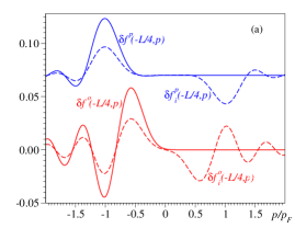
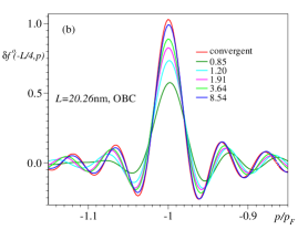
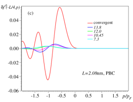
Figure 3: (a) Deviation from equilibrium of the Wigner function at the boundaries $\delta f(-L/4,p)=-\delta f(+L/4,-p)$ for the confined and periodic cases (superscripts $o$ and $p$, respectively) [see the main text and Eq. (8)]; (b, c) The very slow convergence of $\delta f(-L/4,p)$ by increasing all the exact multielectronic eigenstates up to high excitation energies $\Delta\varepsilon=r\varepsilon_{F}$ ($r$ is given in inset) substantially larger than the metallic electrode bandwidth ($\sim\varepsilon_{F}$). Because of rapid oscillations, only the range around the Fermi momentum $p_{F}$ is shown in (b).

In fact, this result is not at all astonishing; on the contrary, it should have been expected. The GDF model is nothing but the continuous version of the discrete model of Eq. (22) of I, for the particular choice $t_{L}=t_{R}=t_{d,L}=t_{d,R}$, $\varepsilon_{L}=\varepsilon_{R}=\varepsilon_{g}$, $U=0$. As seen on the SWF-curve in Fig. 3 of I, at resonance ($\varepsilon_{L}=\varepsilon_{R}=\varepsilon_{g}$), the DG-conductance also vanishes. In this context, what is worth emphasizing is not that the DG approach yields a(n almost) vanishing conductance. In fact, the present calculations confirm the analysis Sect. VI of I that the situation at resonance is particularly favorable for the DG approach to predict a vanishing current. But, as shown in I, $g_{DG}$ can also be nonvanishing. Fig. 3 of I depicted situations where $g_{DG}\neq 0$. But, completely unphysically, as seen in that figure, the farther away from resonance, the larger is the conductance $g_{DG}$. Although more tedious, exact DG calculations are also straightforward for the continuous-space counterpart of the uncorrelated discrete model of I: to this, one should include in Eq. (3) a statical rectangular barrier $v(x)=\varepsilon_{g}\theta(|x|-l)$, wherein $\theta$ is the Heaviside function and $0<l<L/4$.Baldea:unpublished As far as the exact Landauer approach is concerned, the only difference from the uncorrelated model of I is that the Lorentzian decay (cf. Fig. 3 of I) of the exact transmission (Landauer conduction) away from resonance there is replaced by an exponential decays with $\varepsilon_{g}$ and $l$ here.

To demonstrate the failure of the DG approach, we have chosen above the same method pursued in I, of faithfully applying the DG method. Due to its extreme simplicity, the GDF model also offers another alternative decisive way to challenge the DG method. Owing to the fact that the analytical exact scattering solutions of the single particle Schrödinger equation are known for arbitrary $V$, one can pursue a different route. Namely, one should consider small deviations of the single electron wave functions with respect to the exact ones ($\phi_{k}\to\phi_{k}+\delta\phi_{k}$), and investigate their impact on the DG-functional $\mathcal{H}\equiv\langle\Psi|\hat{H}+\hat{W}|\Psi\rangle-\omega\langle\Psi|\Psi\rangle-\sum_{p_{L}>0}\lambda_{p_{L}}\langle\Psi|\hat{F}(q_{L},p_{L})|\Psi\rangle-\sum_{p_{R}<0}\lambda_{p_{R}}\langle\Psi|\hat{F}(q_{R},p_{R})|\Psi\rangle-\sum_{j}\xi_{j}\langle\Psi|\ (\hat{j}(x_{j})-\hat{j}(0))|\Psi\rangle$; it should be minimum if the DG method were correct. That is, one should examine whether $\delta\mathcal{H}=\mathcal{O}(\delta\phi_{k})$ or $\delta\mathcal{H}=+\mathcal{O}((\delta\phi_{k})^{2})$. The expressions thus obtained are somewhat similar to those worked out in our approach of the DG linear response,Baldea:2008b but are obviously no longer limited to the linear response.Baldea:unpublished Moreover, one can thus directly scrutinize the validity of the variational approach itself, by constraining instead of the WF other properties, which are less sensitive to the boundary locations and, highly desirably, have a clearer physical meaning. Thus, one can indeed exploit another “advantage of an analysis based upon an analytical model …” that “avoids issues associated with linear response approximations, perturbation theory, variational methods in a finite basis, specific implementations of electronic structure, or other numerical approximations, thereby allowing a clear focus on the physical assumptions made when using the” DG “method” (cf. Sect. V of GDF).

The results obtained as described above deserve a separate analysis, which is beyond the scope of this Reply. What is important for the present purpose is the unambiguous demonstration that the variational DG method (without any other assumptions) lamentably fails even for the model chosen by GDF themselves.

VI Further issues

In Sect. V, GDF claim that we criticized “the use of a configuration expansion to describe transport properties.” Such a statement cannot be found in I. GDF should not reduce the transport theories based on a configuration expansion (CI) to the DG method. What they actually mean is our clear statement that, even if the DG method were sound, it would be impractical. We showed that even if very many exact eigenstates were included, the current within the DG approach would very slowly converge; for a correlated system, the first 300 exact eigenstates out of a total of 1225 are insufficient. One may think that the convergence is an issue only for correlated systems. Indeed, in correlated systems, for which the DG method was designed, the convergence is extremely poor.

But let us examine the convergence in the uncorrelated GDF model. Because the current (practically) vanishes, let us inspect the quantity $\delta f(q_{L,R},\mp p>0)$ that is directly related to it via time-reversal breaking. To exemplify, along with the convergent results, we present in Figs. 3b and c those obtained by including all exact eigenstates with excitation energies $\Delta\varepsilon$ below a given value $\Delta\varepsilon\leq r\varepsilon_{F}$. Both for sizes where ab initio DG computations were attempted ($L=2$ nm),DelaneyGreer:04a and for those ($L\simeq 20$ nm) where they are hopeless, all exact eigenstates with very high excitation energies ($r\gg 1$) much larger even than the metallic electrode bandwidth ($\sim\varepsilon_{F}$) have to be included to reach convergence. Definitely, this were a serious challenge even for trivial uncorrelated systems and even if this approach were valid. From the perspective of the severe limitations of the number $\mathcal{N}$ of multielectronic configurations in nontrivial ab initio calculations, the very slow convergence of the DG-results observed for the GDF model, for the two models of I, and many others Baldea:unpublished also becomes an important issue because, e. g., increasing $\mathcal{N}$ by $\sim 50$ % at the limit of feasibility and obtaining a change $\sim 3$ % in the investigated properties, one can erroneously conclude that the results almost converged. Indirectly referring to the poor convergence of the DG method demonstrated in I, GDF claimed in Sect. V that “integrated quantities such as the energy may be better approximated compared to local properties such as …current density”. But in reliable transport treatments the convergence is needed just for the latter. Letting alone that, if current conservation were correctly accounted for, the (position-independent) current would also be an “integrated quantity”, $I=L^{-1}\int d\,xj(x)$, let us illustrate the effect of a truncated CI for a case relevant just for the electrode size $L/2\simeq 1$ nm of Ref. DelaneyGreer:04a, . To compare the convergence of the DG method to that of a standard calculation, we consider the change in the total energy caused by $V\neq 0$ in the DG-state, $\Delta E^{DG}\equiv\langle\Psi|\hat{W}|\Psi\rangle$, and in the state $\Psi^{(1)}$ obtained in the first order [$\mathcal{O}(V)$] of the perturbation theory (without any WF- and current-constraints) $\Delta E^{(1)}\equiv\langle\Psi^{(1)}|\hat{W}|\Psi^{(1)}\rangle$. By including all exact eigenstates up to an excitation energy $\Delta\varepsilon=8$ eV, we got within obvious notations $\Delta E^{DG}_{approx}=0.18\Delta E^{DG}_{conv}$ and $\Delta E^{(1)}_{approx}=0.94\Delta E^{(1)}_{conv}$. The convergence is an issue for the DG method, not for a certain particular model. Notice that (i) we considered all aforementioned exact eigenstates, (ii) this $\Delta\varepsilon$-value is four times larger than that of the states considered relevant by DG,DelaneyGreer:04a for which DG mentioned (without any detail) an inaccuracy factor $\sim 3$,DelaneyGreer:04a and (iii) the convergence dramatically deteriorates for a real correlated system. Contrary to DG,DelaneyGreer:04a we cannot see any justified manner to evaluate the inaccuracy factor related to a CI truncation from Figs. 3b and c.

It is obvious that the variational DG approach does not determine the wave function of an eigenstate (cf. Sect. V of GDF), no transport theory should attempt to do this; otherwise, the current would be identically zero unless the systems (e. g., superconductors) sustain persistent currents. We can find neither in Ref. DelaneyGreer:04a, nor elsewhere a mention that the central variational DG ansatz would be an approximation. One deduces that the results are exact if one is able to consider sufficiently large sizes in full CI calculations. This is the case of the uncorrelated discrete model of I. In a valid transport through uncorrelated systems genuinely based on the WF, the current conservation is exact (provided that the Fourier completeness is satisfied if spatial and momentum grids are used).frensley:90 We demonstrated in I that the DG method does not automatically satisfy the current conservation, which needs be explicitly imposed. We did not misinterpret anything, as GDF argue, we criticized the DG claim that this constraint is necessary only for other approaches, which use nonlocal interactions, truncate the molecular orbital basis set or the CI (second paragraph of Sect. VI in I), but not for the DG method, as if that method were so good and automatically accounted for it. The current conservation is trivial, it is satisfied by construction in the calculations where the current is constrained to be position independent, as we also did in I. It is true “that …considerable care is needed in defining finite expansions that are current conserving” (cf. Sect. V of GDF, underlined by us), but this does not affect the results of I, which demonstrate that without explicit imposition, the DG method violates the current conservation: they are deduced within the linear response limit [$\mathcal{O}(V)$] and full CI calculations. One should not confuse the two issues addressed in I: the violation of the current conservation, which is demonstrated by full CI calculations, and the very poor convergence, which is demonstrated by studying (as also done above) the effect of progressively increasing the number of exact eigenstates up to values beyond the reach of any feasible ab initio calculations.

In several places of their Comment, by using the terms “linear response approximation” and “perturbation theory”, GDF indirectly mean criticism to I, e. g. in Sect. V, where they mention “the advantage of an analysis based upon an analytical model …that …avoids issues associated with linear response approximations, perturbation theory …”. GDF should have noted that, as emphasized in Sect. IV, their derivation of $g_{0}$ of Sect. IV.B is also based on the linear response approximation: the difference is that they employ it implicitly and heuristically, while our approach uses a systematic $\mathcal{O}(V)$ expansion spanning the whole Hilbert space (full CI).

The current oscillations mentioned by GDF in Sect. V (which are rather irregular fluctuations Baldea:unpublished ) have neither to do with the simplicity nor with the dimensionality ($d=1$) of the models of I. As noted there, for the uncorrelated model and the sizes considered by us, the time-dependent density matrix renormalization group (t-DMRG) yields the correct physical result, while the DG method lamentably fails either with or without imposing current conservation. Likewise, the correct result is obtained within the standard Keldysh formalism,HaugJauho despite the fact that the electrodes are modeled by the same tight-binding model used in I, and the employed Green functions $G(x,x^{\prime},\varepsilon)$ should have been more affected by “nearsightedness” than the density matrix $\rho(x,x^{\prime})$: they depend not only on the difference $x-x^{\prime}$, but also on energy. The exponent $d$ of the density matrix decay given by GDF is wrong; the correct one is $(1+d)/2$.Taraskin:02 GDF should have also noted that, for their $Au_{13}$- or $Au_{20}$-“electrodes”, each of $L/2\simeq 1$ nm, the spatial variation of the density matrix within $\mathcal{L}\sim$$0.5$ nm (Ref. 20) to which they refer is important, and the invoked “nearsightedness” problematic. Concerning this, noteworthy, the above $\mathcal{L}$-value is deduced by calculating $\rho(x,x^{\prime})$ in very large systems of sizes much longer that $\mathcal{L}$, and not employing short DG-like electrodes, each of $L/2\simeq 1$ nm.

The simple uncorrelated model of I, which is a textbook’s example, correctly describes the major features of nanotransport, if the well-established approaches mentioned above are applied, but not within the DG method. Definitely, the failure is of the DG method itself and has nothing to do with the simplicity of the model. This issue regards the GDF model as well, for which their Landauer-type calculations and ours (cf. Sect. IV) also yield the correct conductance, Kohn’s principle notwithstanding. Of course, Kohn’s principle is relevant for realistic systems, but, curiously, GDF did not note that Kohn’s tight-binding prediction provides the best overall fit of realistic calculations of the density matrix decay, as shown in the work to which they refer (Ref. 20).

Contrary to the GDF’s claim, I is not a comment on the validity of the DG method. In I we simply checked whether the DG method is able to describe the most simple uncorrelated and correlated systems. If we wrote a comment, we would certainly have raised even more questions than on the fundamental issues of the next section. Letting alone minor issues (e. g, the missing value of $V$ in Fig. 1 of Ref. DelaneyGreer:04a, ), we would have asked, e. g., how did DG conceive to apply their method to the Kondo effect (cf. last but one paragraph of Ref. DelaneyGreer:04a, ). For typical Kondo temperatures $T_{K}\sim 1$ mK$-1$ K, this would imply to handle electrodes longer than the Kondo cloud length, $L>\xi_{K}\sim\hbar v_{F}/(k_{B}T_{K})\approx 10^{3}-10^{6}$ nm within a CI expansion capable to very accurately describe a huge number of excited eigenstates, especially the very low excitations related to coherent spin fluctuations of energies $\sim k_{B}T_{K}\sim 10^{-4}-10^{-7}$ eV.

VII Discussion. Why does the variational DG method fail?

As already stressed in Sect. I, in I we criticized the WF-OBCs in the specific context of the variational DG method (which means more than WF-OBCs) and not otherwise. Let us assume that GDF could have demonstrated that the WF-OBCs are correct. What would be the implication on the (in)validity of the DG? None, since our calculations were done just by imposing WF-OBCs (i. e., they were assumed to be “correct”), and the fact that the results obtained within the DG approach presented in I are unphysical remains unaltered. The only implication would be that one could formulate more precisely: the DG method fails not because the WF-OBCs per se are wrong, but because, with these OBCs, imposing one or more conditions prescribed by the DG to determine the steady state is unphysical.

Even if (hypothetically) examples could be found where results of a certain approach (in our case, the DG’s) were acceptable, a single counter-example suffices to demolish it. The results for two examples presented in I as well as those for the GDF model of Sect. V unambiguously demonstrate the lamentable failure of the DG method both for uncorrelated and for uncorrelated transport. This is an irrefutable mathematical demonstration for the simplest correlated and uncorrelated, for discrete and continuum-space models, since their derivation uses nothing else than the variational DG method prescribes. Consequently, the main objective of the present Reply has been achieved.

The problem that is really important is not whether the DG approach fails, but rather why it fails. We do not present here a comprehensive analysis,Baldea:unpublished but for the benefit of a reader interested in this method, we briefly note the following. Besides WF-OBCs, the DG method prescribes the total energy minimization and the usage of a normalized many-electron wave function $\Psi$ to describe a nonvanishing steady state current. Noteworthy, both conditions refer to a finite isolated system. So, within this philosophy, it could be possible to obtain a nonvanishing steady state current, i. e., phenomenon that is manifestly irreversible, by merely examining a cluster which is not only finite (and even very small, cf. Ref. DelaneyGreer:04a, ) but also isolated, by imposing certain constraints at certain (very special) locations inside this cluster. The DG method uses absolutely no other information than that pertaining to a finite isolated system: this system is completely decoupled from the world, and there is absolutely no source of dissipation. At this point, it is important to emphasize that, basically, valid approaches to transport fall into two classes:

(i) Most widely used are transport theories, e. g., based on the Keldysh NEGF or master equations, which also consider a finite cluster (wherein possible electron correlations are treated within DFT or more accurately Ng:88 ; Meir:92 ; HaugJauho ), but this finite cluster is linked to infinite electrodes. It is this latter ingredient that accounts for irreversibility in a physically justifiable manner: the imaginary parts of the embedding (contact) self-energies become nonvanishing only in infinite electrodes.ElectrodeSelfEnergies On the other side, that the DG approach can lead to a nonvanishing current is solely a lucky mathematical consequence: certain matrix elements of the Fano operator (not directly related to an observable with an unequivocal physical meaning, like e. g., the electronic number operator) computed somewhere inside of a finite isolated cluster happen to have nonvanishing imaginary parts, a fact by no means related to a true physical dissipation. Therefore, although by no means critically related with the failure of the DG method demonstrated unambiguously mathematically, we reiterate our claim of I, that imposing WF-OBCs within the DG prescription is not physically justified. WF-OBCs can be used, but within other approaches (e. g., by solving the Liouville equation for the WF frensley:90 ), for which the present considerations do not in the least apply. Consequence of an ad hoc mathematical constraint without a precise physical meaning, the predicted DG current (vanishing or not) exhibits, not concidentally, completely unphysical trends (cf. Sect. V, and Figs. 3 and 7 of I). Summarizing, in this paragraph we have indicated one serious flaw of the DG method.

(ii) Another class of transport treatments deduces the steady-state current by examining the long time ($t\to\infty$) behavior of the wave function $\Psi(t)$ at zero temperature (e. g., the already mentioned t-DMRG) or the statistical (density matrix) operator $\hat{\rho}(t)$ at finite temperatures. AndreiLimits:06 In the former, starting from $x\sim-L/2$ (in the present notations) the many-body wave packet is monitored a sufficiently long time $t$, but before the packet reaches the other end ($x\sim+L/2$), since in the absence of any dissipation it will be reflected, a reversed current will appear, and current oscillations will last forever. Mathematically, this amounts to derive steady-state properties (e. g., electric current) by approaching the limit $L\to\infty$ first, and only then $t\to\infty$. The clear physical analysis of Ref. AndreiLimits:06, explicitly emphasizes the importance of the correct order of these two limits for reaching the steady state; see Eq. (6) there. This represents the counterpart of the fact well known in solid state physics on the calculation of the dc-conductivity $\sigma_{dc}$ from the frequency- and wavevector-dependent conductivity $\sigma(\mathbf{q},\omega)$. To obtain the correct result, it is mandatory to take the limits $\mathbf{q}\to\mathbf{0}$ and $\omega\to 0$ (the counterparts of $L\to\infty$ and $t\to\infty$, respectively) in that order,

$$\sigma_{dc}=\lim_{\omega\to 0}\lim_{\mathbf{q}\to\mathbf{0}}\sigma(\mathbf{q},\omega);$$

see, e. g., chapter 3.8 of Ref. mahan, . The above considerations can be rephrased perhaps in a more direct manner as follows. The current operator $\hat{j}$ does not commute with the hermitian Hamiltonian $\hat{H}$ of a non-dissipative system, and consequently

$$\frac{\partial\hat{j}}{\partial t}=i[\hat{H}(t),\hat{j}(t)]\neq 0.$$

A steady state $\lim_{t\to\infty}\Psi(t)$ characterized by a stationary current

$$\lim_{t\to\infty}\partial I(t)/\partial t=0,\mbox{ and }\lim_{t\to\infty}I(t)=I\neq 0$$

can only be obtained because, after averaging the commutator (a nonvanishing operator), $\langle\Psi|[\hat{H},\hat{j}]|\Psi\rangle_{t}$, the average can vanish if one first takes the infinite “volume” limit $L\to\infty$ and then $t\to\infty$.

In examining a steady state transport, two general principles of the thermodynamics of irreversible processes are mostly discussed in the literature: the minimum entropy production prigogine:49 and the entropy maximization.Jaynes:57b Prigogine’s discussion of the steady state within the former principle prigogine:49 clearly revealed that the aforementioned order of the two limits is essential. Within the same principle, the same fact was nicely illustrated in the particular case of the flow through a capillary tube connecting two containers with ideal gas at different pressures.MinEntropyProduction Were the system finite, the flow would be no more irreversible: after some time, the gas would flow back to higher pressure. In Ref. DelaneyGreer:04a, , DG claimed that they can deduce the variational ansatz, which they used to compute the steady state wave function $\Psi$, from the maximum entropy principle. Except for citing Ref. Jaynes:57a, , neither in Ref. DelaneyGreer:04a, , nor in later works,DelaneyGreer:04b ; DelaneyGreer:06 ; Fagas:07 or in the Comment any detail on this derivation was provided. In Ref. Jaynes:57a, , Jaynes presented quantitative considerations emerging from that principle applied to systems of very large number of degrees of freedom based on Shannon’s entropy for statistical equilibrium; a steady state is not even mentioned. In a subsequent paper,Jaynes:57b cited in a later work by DG,DelaneyGreer:06 Jaynes further analyzed the time-dependent case in detail from the perspective of a single basic principle (entropy maximization) applied to all cases, equilibrium or otherwise. Again, the case of a steady state was not explicitly considered, and consequently the issue of the correct limit order to reach a steady state within the principle of entropy maximization was not addressed. Prior to the DG work, there has been attempted to recover the standard Landauer results from the maximum entropy inference,Bokes:03 and it turned out that schemes based on that principle encounter notable difficulties even if the limits $L\to\infty$ and $t\to\infty$ are taken in the correct order. Ignoring these difficulties and without validating their variational scheme against any well-established theoretical result (as done by us in I), DG put forward an approach, wherein, implicitly, the limit order is exactly opposite to the correct one: they consider a time-independent wave function $\Psi$ (amounting to take $t\to\infty$), and then (by taking the largest cluster it can handle, which is in fact very small) attempt to mimic the limit $L\to\infty$. This was the physical reason why in I we employed the acronym SWF (stationary Wigner function) for what we now called the DG method. Therefore, within this physical context we do not think, contrary to GDF (cf. their Ref. 4), that the term SWF is misleading. Summarizing, in this paragraph we have indicated another serious flaw of the DG method, which represents the fundamental physical reason why it fails.

VIII Conclusion

GDF seem to have realized that their claim is wrong; in Sect. III, they write that our conclusion “that an asymmetric injection of electrons is needed to obtain a current is incorrect, if injection refers to incoming electron momentum distributions…” (underlined by us). However, the above conditional clause does not apply and therefore our critique of I is not in the least affected.

To conclude, in this Reply we have demonstrated that in their Comment GDF could neither show that the critique is incorrect, nor give even a single example where the DG method can correctly describe a transport property. We used their model to complete the evidence on the failure of the DG method presented in I. Letting alone the fundamental reasons against this method (cf. Sect. VII), because the failure of the DG method, DelaneyGreer:04a ; DelaneyGreer:04b ; DelaneyGreer:06 which is a unequivocal mathematical prescription, comprises the simplest uncorrelated and correlated systems described within discrete (Ref. Baldea:2008b, ) and continuum (Sect. V) spaces, it would be a utopia to presume that real systems could be correctly described.

Most importantly for readers interesting in the DG method, we have presented not only further exact results showing that this method fails, but also indicated the basic physical reasons why it fails.

DG argued that their essential ingredient, the variational ansatz, is deduced from the maximum entropy principle. In Ref. Jaynes:57b, cited by DG,DelaneyGreer:06 the author asserted that “if it can be shown that the class of phenomena predictable by maximum-entropy inference differs in any way from the class of experimentally reproducible phenomena, that fact would demonstrate the existence of new laws of physics, not presently known.” This statement may apply to the results deduced within the DG method: neither the prediction of the present Sect. V (a vanishing conductance on resonance), nor a conductance increasing if one moves away from resonance (Fig. 3 of I), or conductance maxima of the Coulomb blockade peaks becoming higher and even exceeding $g_{0}$ with decreasing dot-electrode coupling $t_{d}$ (Fig. 7 of I) have been observed so far. These trends are just opposite to those of the available experiments…, so should one still await the advent of new physical laws in the sense quoted above from Ref. Jaynes:57b, ? Until then, one should not be too surprised if the DG predictions are also at odds with other existing experiments of molecular electronics. Until recently,Reed:09 although being unable to demonstrate that their theory is sound, DG could claim that their method DelaneyGreer:04a produces current values better agreeing with experiment than the other theoretical estimations. The accurate data of the beautiful experiment of Ref. Reed:09, have clearly demonstrated that just the opposite is true. To see this, one can simply compare Fig. 2a of Ref. Reed:09, , Fig. 2 of Ref. DelaneyGreer:04a, , and, e. g., Fig. 4 of Ref. Tomfohr:04, among themselves. For instance, at $V=1;1.5$ volt, the currents in $\mu$A are $\simeq 1.7;6$,Reed:09 $\simeq 0.09;0.13$,DelaneyGreer:04a and $\simeq 6;9.7$.Tomfohr:04 So, without any special fine tuning (e. g., contact geometry), a standard NEGF-DFT approach Tomfohr:04 can reasonably describe the experimental data, while the DG’s cannot.

As a matter of principle, we end by reiterating that whether (un)luckily results obtained within a certain theoretical (DG’s or whatsoever) method (dis)agree with experiment is neither the only nor the decisive point to assess its validity: a comparison with experiment is meaningful only if its physical basis is sound.

The authors acknowledge the financial support for this work provided by the Deutsche Forschungsgemeinschaft.

References

- (1) J. C. Greer, P. Delaney, and G. Fagas, arXiv:0912.3431v1.
- (2) I. Bâldea and H. Köppel, Phys. Rev. B 78, 115315 (2008).
- (3) P. Delaney and J. C. Greer, Phys. Rev. Lett. 93, 036805 (2004).
- (4) P. Delaney and J. C. Greer, Int. J. Quant. Chem. 100, 1163 (2004).
- (5) P. Delaney and J. C. Greer, Proc. Roy. Soc. A 462, 117 (2006).
- (6) G. Fagas and J. C. Greer, Nanotechnology 18, 424010 (4pp) (2007).
- (7) We only refer to this model as the GDF’s as a shorthand. This model was employed to discuss electric transport since the early days of quantum mechanics. See, e. g., Fig. 2a in W. Ehrenberg and H. Hönl, Z. Phys. A 68 289 (1931).
- (8) F. Constantinescu and E. Magyari, Problems in Quantum Mechanics, Pergamon Press, 1985, chapter II, problem 22.
- (9) H. Song, Y. Kim, Y. H. Jang, H. Jeong, M. A. Reed, and T. Lee, Nature 462, 1039 (2009).
- (10) I. Bâldea (unpublished).
- (11) The employed numerical -values do not represent special choices; their slight deviations from an integer only reflect the fact that (electron number) should be an integer.
- (12) G. D. Mahan, Many-Particle Physics, Plenum Press, New York and London, second edition, 1990.
- (13) W. R. Frensley, Rev. Mod. Phys. 62, 745 (1990).
- (14) S. Datta, Electronic Transport in Mesoscopic Systems, Cambridge Univ. Press, 1997.
- (15) Unlike in the sound Landauer approach, wherein the linear and nonlinear response can be deduced analytically, DG-calculations must be performed numerically even within the linear response limit.
- (16) Attempts to change the - and -grids used to constrain the boundary WF and the current only yield irrelevant changes in the DG-conductance. For various grid choices [uniform grids, omission of some -points around or where “wildly” varies, use of the grids indicated by Frensley frensley:90 to satisfy the Fourier completeness (although not necessary, because integrations over the continuous are done analytically), etc], one gets -values ranging from .
- (17) H. Haug and A.-P. Jauho, Quantum Kinetics in Transport and Optics of Semiconductors, volume 123, Springer Series in Solid-State Sciences, Berlin, Heidelberg, New York, 1996.
- (18) S. N. Taraskin, P. A. Fry, X. Zhang, D. A. Drabold, and S. R. Elliott, Phys. Rev. B 66, 233101 (2002).
- (19) T. K. Ng and P. A. Lee, Phys. Rev. Lett. 61, 1768 (1988).
- (20) Y. Meir and N. S. Wingreen, Phys. Rev. Lett. 68, 2512 (1992).
- (21) D. S. M. C. Desjonquères, Concepts in Surface Physics, Springer-Verlag, Berlin, 1993.
- (22) B. Doyon and N. Andrei, Phys. Rev. B 73, 245326 (2006).
- (23) I. Prigogine, Physica 15, 272 (1949).
- (24) E. T. Jaynes, Phys. Rev. 108, 171 (1957).
- (25) M. J. Klein and P. H. E. Meijer, Phys. Rev. 96, 250 (1954).
- (26) E. T. Jaynes, Phys. Rev. 106, 620 (1957).
- (27) P. Bokes and R. W. Godby, Phys. Rev. B 68, 125414 (2003).
- (28) J. Tomfohr and O. F. Sankey, J. Chem. Phys. 120, 1542 (2004).