The State of Self-Organized Criticality of the Sun During the Last Three Solar Cycles. I. Observations

Abstract

We analyze the occurrence frequency distributions of peak fluxes $P$, total fluxes $E$, and durations $T$ of solar flares over the last three solar cycles (during 1980–2010) from hard X-ray data of HXRBS/SMM, BATSE/CGRO, and RHESSI. From the synthesized data we find powerlaw slopes with mean values of $\alpha_{P}=1.72\pm 0.08$ for the peak flux, $\alpha_{E}=1.60\pm 0.14$ for the total flux, and $\alpha_{T}=1.98\pm 0.35$ for flare durations. We find a systematic anti-correlation of the powerlaw slope of peak fluxes as a function of the solar cycle, varying with an approximate sinusoidal variation $\alpha_{P}(t)=\alpha_{0}+\Delta\alpha\cos{[2\pi(t-t_{0})/T_{cycle}]}$, with a mean of $\alpha_{0}=1.73$, a variation of $\Delta\alpha=0.14$, a solar cycle period $T_{cycle}=12.6$ yrs, and a cycle minimum time $t_{0}=1984.1$. The powerlaw slope is flattest during the maximum of a solar cycle, which indicates a higher magnetic complexity of the solar corona that leads to an overproportional rate of powerful flares.

1 Introduction

In the observational part of this study (Paper I) we focus on the statistics of solar-flare hard X-ray fluxes during the course of the last three solar cycles, while theoretical modeling is referred to Paper II. Solar flares are catastrophic events in the solar corona, most likely caused by a magnetic instability that triggers a magnetic reconnection process, producing emission in almost all wavelengths. Since the emission mechanisms are all different in each wavelength, such as nonthermal bremsstrahlung (in hard X-rays), thermal bremsstrahlung and free-bound or recombination radiation (in soft X-rays and EUV), gyrosynchrotron emission (in microwaves), plasma emission (in metric and decimetric waves), etc. , estimates of the energy contained in each flare event strongly depends on the emission mechanism, and thus on the wavelength. In this study we concentrate on the hard X-ray wavelength. Hard X-ray emission in solar flares mostly results from thick-target bremsstrahlung of nonthermal particles accelerated in the corona that precipitate into the dense chromosphere. Thus, the hard X-ray flux is the most direct measure of the energy release rate, and thus is expected to characterize the energy of flare events in a most uncontaminated way, while emission in other wavelengths exhibit a more convolved evolution of secondary emission processes. The main observables that are available for flare statistics in hard X-rays are the peak flux $P$, the total flux or fluence $E$ (defined as the time-integrated flux over the entire event), and the total time duration $T$ of the event. In this study, we present a comprehensive compilation of occurrence frequency distributions of these observables obtained in hard X-rays, and investigate whether their behavior is different during solar cycle minima, including the current anomalous solar minimum.

2 Statistics of Solar Flares in Hard X-rays

In this Section we describe observed occurrence frequency distributions of solar flare hard X-ray parameters (in chronological order), discuss the properties of the datasets (hard X-ray energies, observational epochs, instruments), compile the results in Table 1 (powerlaw slopes of fluxes, fluences, durations, number of events, instruments, and references), and derive synthesized distributions that serve as reference values of the average solar flare activity. In a subsequent Section we investigate whether deviations from these reference values can be found during the solar cycle.

Table 1.: Frequency distributions measured from solar flares in hard X-rays and gamma-rays. References: ¹) Datlowe et al. (1974); ${}^{2})$ Lin et al. (1984); ${}^{3})$ Dennis (1985); ${}^{4})$ Schwartz et al. (1992); ${}^{5})$ Crosby et al. (1993); ${}^{6})$ Biesecker et al. (1993); ${}^{7})$ Biesecker et al. (1994); ${}^{8})$ Crosby (1996); ${}^{9})$ Lu et al. (1993); ${}^{10})$ Lee et al. (1993); ${}^{11})$ Bromund et al. (1995); ${}^{12})$ Perez Enriquez and Miroshnichenko (1999); ¹³ Su et al. (2006); ¹⁴ Christe et al. (2008); ${}^{15})$ Lin et al. (2001); ${}^{16})$ Tranquille et al. (2009).

Powerlaw	Powerlaw	Powerlaw	Number	Instrument	Reference
slope of	slope of	slope of	of	and
peak flux	fluence	durations	events	threshold
$\alpha_{P}$	$\alpha_{E}$	$\alpha_{T}$	$n$	energy
1.8			123	OSO–7($>$20 keV)	1)
2.0			25	UCB($>$20 keV)	2)
1.8			6775	HXRBS($>$20 keV)	3)
1.73$\pm$0.01			12,500	HXRBS($>$25 keV)	4)
1.73$\pm$0.01	1.53$\pm$0.02	2.17$\pm$0.05	7045	HXRBS($>$25 keV)	5)
1.71$\pm$0.04	1.51$\pm$0.04	1.95$\pm$0.09	1008	HXRBS($>$25 keV)	5)
1.68$\pm$0.07	1.48$\pm$0.02	2.22$\pm$0.13	545	HXRBS($>$25 keV)	5)
1.67$\pm$0.03	1.53$\pm$0.02	1.99$\pm$0.06	3874	HXRBS($>$25 keV)	5)
1.61$\pm$0.03			1263	BATSE($>$25 keV)	4)
1.75$\pm$0.02			2156	BATSE($>$25 keV)	6)
1.79$\pm$0.04			1358	BATSE($>$25 keV)	7)
1.59$\pm$0.02		2.28$\pm$0.08	1546	WATCH($>$10 keV)	8)
1.86	1.51	1.88	4356	ISEE–3($>$25 keV)	9)
1.75	1.62	2.73	4356	ISEE–3($>$25 keV)	10)
1.86$\pm$0.01	1.74$\pm$0.04	2.40$\pm$0.04	3468	ISEE–3($>$25 keV)	11)
1.80$\pm$0.01	1.39$\pm$0.01		110	PHEBUS($>$100 keV)	12)
1.80$\pm$0.02		2.2$\pm$1.4	2759	RHESSI($>$12 keV)	13)
1.58$\pm$0.02	1.7$\pm$0.1	2.2$\pm$0.2	4241	RHESSI($>$12 keV)	14)
1.6			243	BATSE($>$8 keV)	15)
1.61$\pm$0.04			59	ULYSSES($>$25 keV)	16)

One of the earliest reports of a frequency distribution of solar hard X-ray flare fluxes was made by Datlowe et al. (1974), who published a frequency distribution of 123 flare events detected in the 20–30 keV energy range above a threshold of $\lower 1.72218pt\hbox{$\;\buildrel>\over{\scriptstyle\sim}\;$}0.1$ photons (cm^-2 s^-1 keV^-1) with the OSO–7 spacecraft during the period of 10 October 1971 – 6 June 1972, finding a powerlaw slope of $\beta_{P}\approx 0.8$ for the cumulative frequency distribution. For compatibility we list only powerlaw slopes $\alpha$ of differential frequency distributions in Table 1, and use the conversion $\alpha=\beta+1$ when needed. We list also the number of events, which is a good indicator of the statistical uncertainty of the powerlaw slope fits (Figure 6).

A sample of 25 microflares of smaller size were detected at 20 keV with a balloon-borne instrumentation of University of California Berkeley (UCB) during 141 minutes of observations on 27 June 1980, yielding a powerlaw distribution with a slope of $\beta\approx 1$ (Lin et al. 1984).

Many more events were observed with the Hard X-Ray Burst Spectrometer (HXRBS) onboard the Solar Maximum Mission (SMM) spacecraft, which recorded 6775 flare events during the 1980–1985 period, exhibiting a powerlaw distribution of peak count rates with a slope of $\alpha_{P}=1.8$, extending over four orders of magnitude (Dennis 1985).

A next mission with hard X-ray detector capabilities was the Compton Gamma Ray Observatory (CGRO). Although it was designed to detect gamma-rays from astrophysical objects, it also detected solar flares systematically during the period of 1991–2000. Using the Burst And Source Transient Experiment (BATSE), statistics of flares with energies $>25$ keV was sampled and more detailed powerlaw distributions of peak fluxes were reported with values of $\alpha_{P}=1.61\pm 0.03$ (Schwartz et al. 1992), $\alpha_{P}=1.75\pm 0.02$ (Biesecker et al. 1993), and $\alpha_{P}=1.79\pm 0.04$ (Biesecker et al. 1994) for BATSE. Biesecker (1994) noticed slight differences of the powerlaw slope during low activity $(\alpha_{P}=1.71\pm 0.04$) and high activity periods ($\alpha_{P}=1.68\pm 0.02$), with the powerlaw slope usually flatter for high-activity periods.

A systematic study of flares observed with HXRBS over the entire mission duration of 1980–1989 was conducted by Crosby et al. (1993), measuring peak count rates $P_{cts}$ (cts s^-1), converted into photon fluxes $P_{ph}$ (photons cm^-2 s^-1 keV^-1) at energies $>25$ keV, peak HXR spectrum-integrated fluxes $P_{X}$ (photons cm^-1 s${}^{-1})$, peak electron fluxes $P_{e}$ (ergs s^-1), flare durations $T$, and time-integrated total energies in electrons $E_{e}$ (ergs), for four different time intervals of the solar cycle. In Table 1 we list the values for the time ranges of 1980–1982 (7045 events; solar maximum phase), 1983–1984 (1008 events), 1985-1987 (545 events; solar minimum phase), and 1988-1989 (3874 events). The values of the powerlaw slopes change by $\lower 1.72218pt\hbox{$\;\buildrel<\over{\scriptstyle\sim}\;$}2\%$ during different periods of the solar cycle.

From the Wide Angle Telescope for Cosmic Hard X-Rays (WATCH) onboard the Russian satellite GRANAT, a sample of 1546 flare events was observed at energies of 10–30 keV during 1990–1992, yielding similar powerlaw slopes for peak count rates, $\alpha_{P}=1.59\pm 0.02$, and flare durations $\alpha_{T}=2.28\pm 0.08$ as reported before (Crosby, 1996; Crosby et al. 1998). However, it was noted that the frequency distribution of flare durations exhibits a gradual rollover for short flare durations, approaching a slope of $\alpha_{T}\approx 1$, so it cannot be fitted with a single powerlaw distribution over the entire range of flare durations. From the PHEBUS instrument on GRANAT, which is sensitive to gamma-ray energies, Perez Enriquez and Miroshnichenko (1999) analyzed 110 high-energy solar flares observed in the energy range of 100 keV – 100 MeV and found the following powerlaw slopes: $\alpha_{P}=1.80\pm 0.01$ for (bremsstrahlung) hard X-ray fluxes at $>100$ keV, $\alpha_{P}=1.38\pm 0.01$ for photon energies at 0.075 – 124 MeV, $\alpha_{P}=1.39\pm 0.01$ for bremsstrahlung at 300 – 850 keV, $\alpha_{E}=1.50\pm 0.03$ for the 511 keV annihilation line fluence, $\alpha_{E}=1.39\pm 0.02$ for the 2.223 MeV neutron line fluence, and $\alpha_{E}=1.31\pm 0.01$ for the 1 – 10 MeV gamma-ray line fluence. The flatter powerlaw slopes of the occurrence frequency distributions at higher energies could possibly be explained by flatter spectra (Section 3.1).

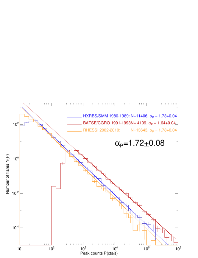
Figure 1.: Occurrence frequency distributions of hard X-ray peak count rates $P$ (cts/s) observed with HXRBS/SMM (1980 – 1989), BATSE (1991 – 1993), and RHESSI (2002 – 2010), with powerlaw fits. An average pre-flare background of $40$ cts s^-1 was subtracted from the HXRBS count rates. Note that BATSE/CGRO has larger detector areas, and thus records higher count rates.

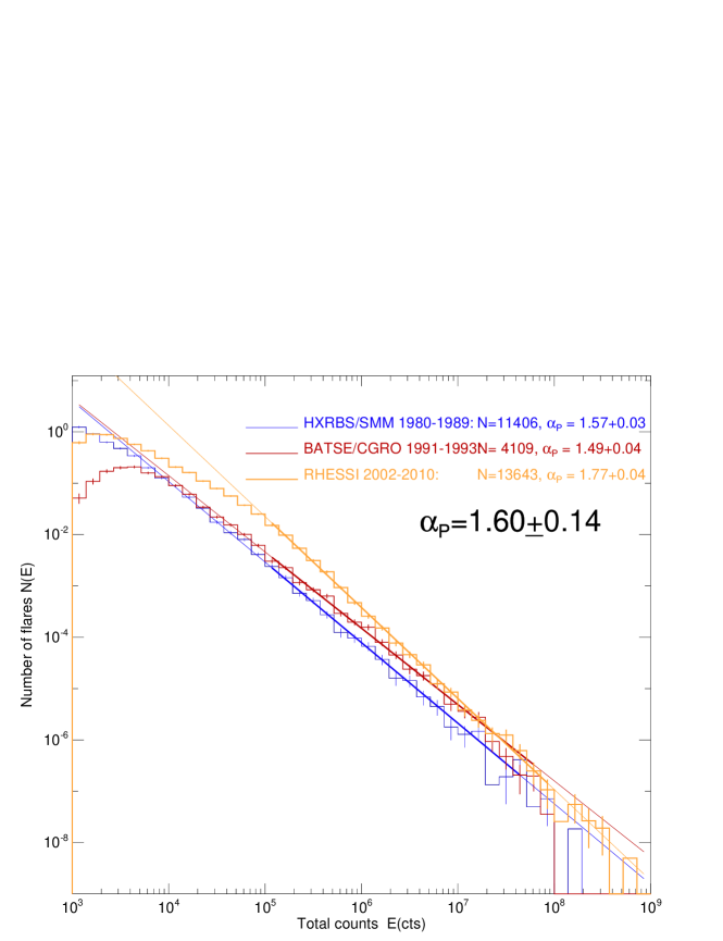
Figure 2.: Occurrence frequency distributions of hard X-ray total counts or fluence $E$ (cts) observed with HXRBS/SMM (1980 – 1989), BATSE (1991 – 1993), and RHESSI (2002 – 2010), with powerlaw fits. An average pre-flare background of $40$ cts s^-1 mulitplied with the flare duration was subtracted in the total counts of HXRBS.

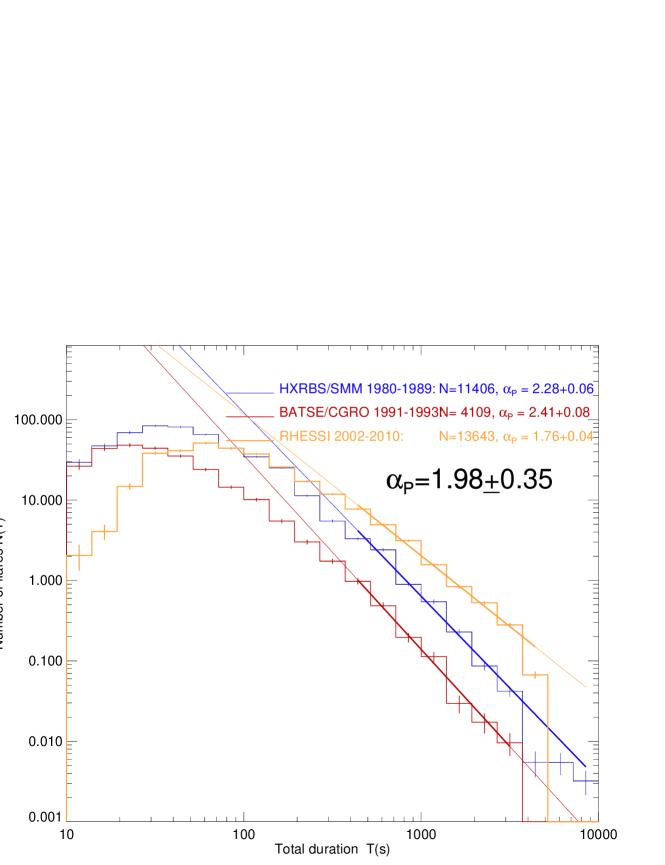
Figure 3.: Occurrence frequency distributions of hard X-ray flare durations $T(s)$ observed with HXRBS/SMM (1980 – 1989), BATSE (1991 – 1993), and RHESSI (2002 – 2010), with powerlaw fits. The flare durations for RHESSI were estimated from the time difference between the start and peak time, because RHESSI flare durations were determined at a lower energy of 12 keV (compared with 25 keV for HXRBS and BATSE), where thermal emission prolonges the nonthermal flare duration.

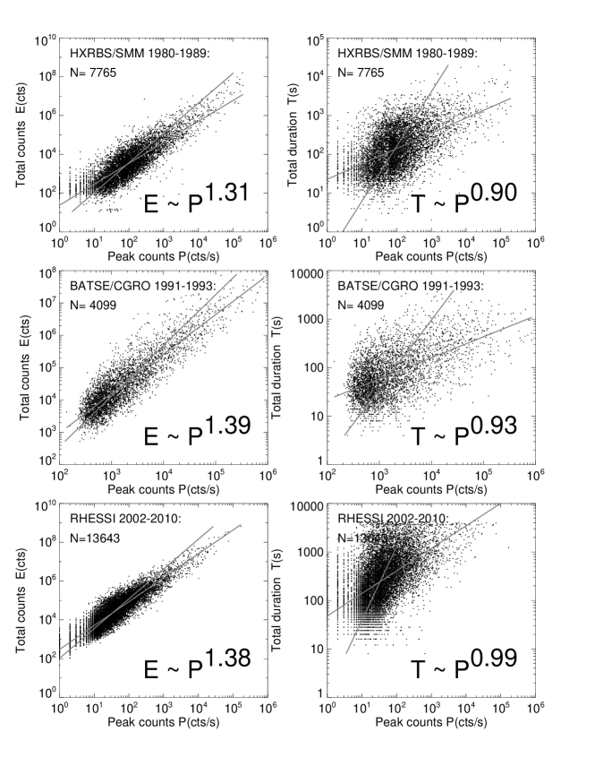
Figure 4.: Scatterplots between the total counts $E(P)$ (left panels) or flare duration $T(P)$ (right panels) versus the peak count rate $P$ for solar flares with HXRBS/SMM (1980 – 1989) (top), BATSE/CGRO (1991 – 1993) (middle), and RHESSI (2002 – 2010) (bottom). Linear regression fits are applied for $y(x)$ and $x(y)$ (grey lines) and the listed values correspond to the average of the two linear regression fits.

Using data from a $>25$ keV hard X-ray detector onboard the ISEE–3/ICE spacecraft during 24 August 1978 and 11 July 1986, Lu et al. (1993) determined the frequency distributions of the peak luminosity $P$ (erg s${}^{-1})$, the energy $E$ (erg), and flare duration $T$ (s) and found that the measured distributions could be best fitted with a cellular automaton model that produced powerlaw slopes of $\alpha_{P}=1.86$, $\alpha_{E}=1.51$, and $\alpha_{T}=1.88$. The fits of the distributions included an exponential rollover at the upper end, which explains why they inferred a less steep slope for durations than previously reported. Lee et al. (1993) analyzed the same data and determined the correlations and frequency distribution powerlaw slopes with special care of truncation biases and obtained similar values for ISEE–3 ($\alpha_{P}=1.75$, $\alpha_{E}=1.62$, $\alpha_{T}=2.73$) as Crosby et al. (1993) for HXRBS. A third study was done with the same data (Bromund et al. 1995), where the energy spectrum was also calculated to determine different energy parameters, similar to the study of Crosby et al. (1993), finding the following powerlaw slopes: $\alpha_{P}=1.86,...,2.00$ for the peak photon flux $P_{ph}$ (photons cm^-2 s^-1), $\alpha_{P}=1.92,...,2.07$ for the peak electron power $P_{e}$ (erg s^-1), $\alpha_{E}=1.67,...,1.74$ for the total electron energy $E_{e}$ (erg), and $\alpha_{T}=2.40,...,2.94$ for the total duration $T$ (s), where the range of powerlaw slopes results from the choice of the fitting range. The flare duration $T$ was defined at a level of 1/e times the peak count rate.

From the latest solar mission with hard X-ray capabilities, the Ramaty High-Energy Solar Spectroscopic Imager (RHESSI) spacecraft, frequency distributions were determined in the 12 – 25 keV energy band from 2002 – 2005 (Su et al. 2006), finding powerlaw slopes of $\alpha_{P}=1.80\pm 0.02$ for the peak fluxes, and a broken powerlaw $\alpha_{T}$=0.9 – 3.6 for the flare duration, similar to previous findings (e.g., Crosby et al. 1998). Christe et al. (2008) conducted a search of microflares and identified a total of $\approx 25,000$ events observed with RHESSI during 2002 – 2007 and investigated the frequency distributions at lower energies, finding powerlaw slopes of $\alpha_{P}=1.50\pm 0.03$ for 3 – 6 keV peak count rates $P_{ph}$ (cts s^-1), $\alpha_{P}=1.51\pm 0.03$ for 6 – 12 keV peak count rates, and $\alpha_{P}=1.58\pm 0.02$ for 12 – 25 keV peak count rates. Converting the peak count rates $P$ into total energy fluxes by integrating their energy spectra, Christe et al. (2008) find an energy distribution with a powerlaw slope of $\alpha_{E}=1.7\pm 0.1$, with an average energy deposition rate of $\lower 1.72218pt\hbox{$\;\buildrel<\over{\scriptstyle\sim}\;$}10^{26}$ erg s^-1. It is interesting that this microflare statistics is fairly consistent with overall flare statistics, even though it represents only a subset in the lowest energy range.

Flare statistics was also gathered from the Solar X-ray/Cosmic Gamma-Ray Burst Experiment (GRB) onboard the Ulysses spacecraft (Tranquille et al. 2009), finding similar results for $>25$ keV events, i.e. , a powerlaw slope of $\alpha_{P}=1.60\pm 0.04$, which steepens to $\alpha_{P}=1.75\pm 0.08$ if the largest events with pulse pile-up are excluded.

We re-compiled statistics from existing flare catalogs from the three instruments HXRBS/SMM (1980 – 1989), BATSE/CGRO (1991 – 1993), and RHESSI (2002 – 2010) and show summary plots of the resulting frequency distributions in Figures 1–3. The powerlaw slopes are obtained from weighted linear regression fits, using the Poisson statistics of the number of events in each logarithmic bin (see Section 3.5). The average powerlaw slope for peak fluxes $P$ is $\alpha_{P}=1.72\pm 0.08$ (Figure 1). The corresponding frequency distributions of total counts or fluences are shown in Figure 2, which have an average powerlaw slope of $\alpha_{E}=1.60\pm 0.14$ in the range of $E\geq 10^{5}$ cts. The distributions of flare durations are shown in Figure 3, which exhibit an average of $\alpha_{T}=1.98\pm 0.35$, with a tendency of a rollover at the low end. Thus, our synthesized reference values are,

$$\begin{array}[]{ll}N(P)\propto P^{-\alpha_{P}}&\alpha_{P}=1.72\pm 0.08\\ N(E)\propto E^{-\alpha_{E}}&\alpha_{E}=1.60\pm 0.14\\ N(T)\propto T^{-\alpha_{T}}&\alpha_{T}=1.98\pm 0.35\\ \end{array}$$

which are compatible with most of the published values listed in Table 1. Thus, we can consider these synthesized values as representative means, averaged from three major missions over the last 30 years and three solar cycles, which can serve as a reference for the overall flare productivity of the Sun in hard X-ray wavelengths.

In Figure 4 we show the correlation plots between the parameters (sampled in Figures 1 – 3) and determine linear regression fits, which yield scaling laws of $E\propto P^{1.36\pm 0.04}$ and $T\propto P^{0.94\pm 0.05}$. Theoretically, these correlation coefficients can also be calculated from the powerlaw slopes of the frequency distributions. If two parameters $x$ and $y$ have powerlaw distributions $N(x)\propto x^{-\alpha_{x}}$ and $N(y)\propto y^{-\alpha_{y}}$, and the parameters are correlated by a powerlaw relationship $y\propto x^{\beta}$, the powerlaw indices are related by $\beta=(\alpha_{x}-1)/(\alpha_{y}-1)$ (e.g., Aschwanden 2010a; Section 7.1.6). Therefore, based on the powerlaw slopes $\alpha_{P}$, $\alpha_{E}$, and $\alpha_{T}$ measured in Figures 1–3, we expect the following correlations between these three parameters,

$$\begin{array}[]{ll}E\propto P^{\beta_{E}}&\beta_{E}={(\alpha_{P}-1)/(\alpha_{E}-1)}={(1.72-1)/(1.60-1)}=1.2\pm 0.2\\ T\propto P^{\beta_{T}}&\beta_{T}={(\alpha_{P}-1)/(\alpha_{T}-1)}={(1.72-1)/(1.98-1)}=0.8\pm 0.2\\ \end{array}$$

The correlation plots shown in Figure 8, where the linear regression fit is performed for $y(x)$ with $x$ as independent variable, as well as for $x(y)$ with $y$ as independent variable, respectively. The averaged powerlaw slopes (of both linear regression fits and all three datasets) yield values of $E\propto P^{1.36\pm 0.04}$ and $T\propto P^{0.94\pm 0.05}$, which are fully consistent with the values derived from the powerlaw slopes of the frequency distributions (Eq. 2), i.e., $E\propto P^{1.2\pm 0.2}$ and $T\propto P^{0.8\pm 0.2}$.

3 Uncertainties and Errors of Powerlaw Slopes

The determination of powerlaw slopes and their uncertainties are subject to methodical and data selection effects. Given the variation of observed powerlaw slopes as listed in Table 1, it might be useful to briefly discuss some important selection effects and statistical uncertainties.

3.1 Energy or Wavelength Bias

In Table 1 we compare mostly flare data in the hard X-ray regime with energies of $>20$ keV or $>25$ keV, which all have similar powerlaw slopes of $\alpha_{P}\approx 1.6-1.8$. Even flares detected at lower energies $>8$ keV (Lin et al. 2001) or $>12$ keV (Su et al. 2006; Christe et al. 2008) have similar powerlaw slopes. On the other end, flares detected at high energies of $>100$ keV (Perez Enriquez and Miroshnichenko 1999) have also similar powerlaw slopes. However, the same subset of flares observed at 0.075 – 124 MeV, from bremsstrahlung at 300 – 850 keV, from the 511 keV annihilation line fluence, from the 2.223 MeV neutron line fluence, and from the 1 – 10 MeV gamma-ray line fluence, have significantly flatter powerlaw slopes ($\alpha_{P}\approx 1.3-1.4$). This can be explained by the flatter energy spectra of large flares, which causes relatively higher fluxes at higher energies, and thus flatter occurrence frequency distributions. Dennis (1985) has shown a systematic tendency of the hard X-ray spectrum as a function of the hard X-ray count rate, being generally flatter for large flares with high count rates, which predicts also flatter powerlaw slopes of the occurrence frequency distributions at higher energies. Similar wavelength bias effects occur also for flare fluxes detected in soft X-rays and EUV wavelengths, compared with hard X-ray fluxes, which depend on the physical emission mechanism. Therefore we confine our comparisons in Table 1 only to hard X-ray energies in the range of $>8$ keV to $>100$ keV here.

3.2 Effects of Data Gaps and Spacecraft Orbits

Data gaps due to spacecraft night or South Atlantic Anomaly (SAA) passages can also cause systematic biases, because they tend to shorten flare durations (due to interruption) and underestiamte the total flare counts (due to incomplete sampling). These effects can in principle be simulated and their systematic effects on frequency distributions can be quantified this way. Numerical simulations of such selection and instrumental effects are also discussed in the context of waiting time distributions (e.g. , Aschwanden and McTiernan 2010). The distribution of peak fluxes is less affected by data gaps, as long as the peak of a flare is observed. Visual screening of flare light curves was carried out for events detected with HXRBS/SMM, so that missed flare peaks could be identified in the flare catalog (Dennis, private communication). For RHESSI flare catalogs, however, no correction for spacecraft night datagaps has been applied to flare peak fluxes and fluences so far, and long-duration flares are counted multiple times for each spacecraft orbit (McTiernan, private communication).

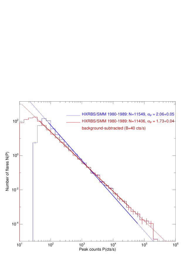
Figure 5.: Occurrence frequency distributions of hard X-ray peak count rates $P$ (cts/s) observed with HXRBS/SMM (1980 – 1989), without background subtraction ($\alpha_{P}=2.06\pm 0.05$; blue), and with subtraction of an average background of $B=40$ cts s^-1 ($\alpha_{P}=1.73\pm 0.01$; red).

3.3 Pre-Event Background Subtraction

Most flare catalogs list the peak counts of flares without preflare background subtraction, which has little impact on large flares, but leads to a strong overestimate of fluxes for the samllest flares, and thus systematically overestimates the powerlaw slope. We demonstrate this for the dataset of HXRBS/SMM flares. Figure 5 shows two (weighted) powerlaw fits, a steeper slope of $\alpha_{P}=2.06\pm 0.05$ for the uncorrected flare peak counts, and a flatter slope of $\alpha_{P}=1.73\pm 0.04$ after subtraction of an estimated average background of 40 cts s^-1. This correction was also applied in the original analysis in Crosby et al. (1993) and we use it here too. Note that the background-uncorrected distribution shows also a steepening of the powerlaw slope at the lower end.

For the RHESSI flare catalog, the preflare background is estimated to be $\approx 10-20$ cts s^-1 per detector, the low limit applying to low spacecraft latitude, the high limit for high latitutes, with a mean of $\approx 12$ cts s^-1 per detector (Jim McTiennan, private communication).

The subtraction of an average preflare background value is only a first-order correction, which may cause even events with negative peak fluxes when the background is time-varying. The optimum method would be to measure the preflare background for each event separately and to subtract it from the peak fluxes, as well as from the fluences before time integration.

3.4 Instrument Sensitivity

The instrumental sensitivity usually translates into a fixed flux threshold, which causes a sharp lower cutoff for peak flux distributions (Figures 1 and 5), but a gradual roll-over for total fluence and duration of events (Figure 2 and 3). The roll-over limits the scale-free range of the distribution over which a powerlaw can be fitted, and moreover produces a systematic bias for flatter powerlaw slopes when part of the roll-over is included in the powerlaw fit. If powerlaw fits are weighted by the number of events per bin in a linear regression fit to a histogram, the lowest bins will have the hightest weight, and thus a gradual roll-over at the lower end will produce a too flat powerlaw slope, when compared with the fit in the upper bins of the distribution. We determine the lower bound of the powerlaw fit range by the $\chi^{2}$-criterion, which reliably detects a roll-over by an excessive deviation from a powerlaw fit in terms of the expected standard deviation.

3.5 Linear Regression Fit Methods

A common method to determine powerlaw slopes is a linear regression fit to a histogram in a $log(N)-log(S)$ diagram, which can be done in two ways. If the frequency distribution closely follows a powerlaw function, a weighted linear regression fit can be performed in log-log space, using the number of events per bin as relative weights. However, if the frequency distribution exhibits significant deviations from a straight powerlaw (e.g. , Figures 2 and 3), a weighted powerlaw fit can only be performed in a powerlaw-like subinterval. Often an unweighted fit (with equal weight in log-log space) is carried out in such cases in order to obtain an approximate powerlaw slope. For the results given in literature (as compiled in Table 1), it is not always clear whether the authors performed a weighted or unweighted linear regression fit, which may significantly deviate from each other depending on the fitted interval. In this study here, we perform only weighted fits in well-defined intervals as described below.

In a log-log histogram, the bins $\Delta x_{i}$ are chosed to be equidistant on a log-scale, but they are exponentially increasing on a linear scale. If $N(x)\approx x^{-\alpha}$ is the fitted powerlaw function, the number of events $N_{i}$ per bin is,

$$N_{i}=\int_{x_{i}}^{x_{i}+\Delta x_{i}}N(x)dx\approx N(x_{i})\Delta x_{i}\ .$$

The statistical uncertainty $\sigma_{i}^{log}$ in bin $\Delta x_{i}$ due to Poisson statistics is then on a log-scale,

$$\sigma_{i}^{log}=\log(N_{i}+\sqrt{N_{i}})-\log(N_{i})\ ,$$

and the statistical weighting factor $w_{i}$ for a linear regression fit that minimizes the squared standard deviations $\sigma_{i}^{log}$ in log-log space is then,

$$w_{i}={1\over[\sigma_{i}^{log}]^{2}}\ .$$

The linear regression fit in log-log space finds then the following best-fit powerlaw function,

$$log(N_{i}^{fit})=N_{0}+\alpha\log(x_{i})\ ,$$

A criterion for the goodness of a fit is the $\chi^{2}$-test, expressed with the so-called reduced $\chi^{2}$-value, which expresses the mean deviation of the data points from the fitted function in units of expected standard deviations,

$$\chi_{red}=\left[{1\over(n-n_{free})}\sum_{i=1}^{n}{(N_{i}-N_{i}^{fit})^{2}\over(\sigma_{i}^{log})^{2}}\right]^{1/2}\ ,$$

where $n$ is the number of datapoints (or histogram bins here) and $n_{free}$ is the number of free parameters of the fitted function, which is $n_{free}=2$ for a linear regression fit (with free parameters $N_{0}$ and $\alpha$ in Eq. 6). However, since the upper part of the histogram in log-log distributions generally include bins with zero or very few events, the validity of Poisson statistics $\sqrt{N_{i}}$ is hampered for $N_{i}\lower 1.72218pt\hbox{$\;\buildrel<\over{\scriptstyle\sim}\;$}10$ and has to be replaced by C-statistics (Cash 1979), which has the following expression corresponding to the reduced $\chi^{2}$-criterion,

$$\chi_{cash}=\left[{2\over(n-n_{free})}\sum_{i=1}^{n}N_{i}\ln(N_{i}/N_{i}^{fit})-(N_{i}-N_{i}^{fit})\right]^{1/2}\ ,$$

where $N_{i}^{fit}$ is the theoretical expectation value based on the best-fit powerlaw function and has to be positive for all fitted bins. For an acceptable powerlaw fit, a value of $\chi_{Cash}\approx 1.0$ is expected. The linear regression fit yields then a powerlaw slope $\alpha$ and the probable uncertainty $\sigma_{\alpha}$ due to Poisson statistics, or C-statistics, respectively.

Figure 6.: Monte-Carlo simulations of powerlaw distributions are carried out for a theoretical powerlaw slope of $\alpha=1.75$ with different random representations according to Equation 11. A single distribution based on $N=1000$ events is shown with powerlaw fit $\alpha=1.73$ (top left panel). The Gaussian distribution of powerlaw slopes obtained from $N_{run}=1000$ runs with different random representations yields a mean of $\alpha=1.74\pm 0.03$ (top right). These Monte-Carlo simulations are repeated for various number of events $N=10^{2},...,10^{5}$, which show a convergence to the mean value and standard deviations towards the theoretical value $\alpha=1.75$ (bottom left). The scaling of the uncertaingy $\delta\alpha(N)$ as a function of the number of events $N$ is also shown (bottom right).

3.6 Monte-Carlo Simulations of Powerlaw Uncertainty

An alternative method to infer the uncertainty of powerlaw slopes is a Monte-Carlo simulation of generating a powerlaw distribution. Mathematically, a desired distribution function $f(x)$ can be generated from uniformly distributed random values $\rho$ in the range of $[0,1]$ by using the inverse function $F^{-1}(x)$ of the integral function $F(x)$ of $f(x)$. Here we wish to generate a frequency distribution of energies $E$ in the form of a powerlaw function $p(E)$ with slope $\alpha$ (Aschwanden 2010a, Section 7.1.5),

$$p(E)=(\alpha-1)E^{-\alpha}\ ,$$

which fulfills the normalization $\int_{1}^{\infty}p(E)dE=1$. The total probability $\rho(E)$ in the range $[0,E]$ is then the integral function of $p(E)$ (Eq. 9),

$$\rho(E)=\int_{0}^{E}p(\epsilon)d\epsilon=\int_{0}^{E}(\alpha-1)\epsilon^{-\alpha}d\epsilon=\left[1-E^{(1-\alpha)}\right]\ .$$

The inverse function $E(\rho)$ of $\rho(E)$ (Eq. 10) is

$$E(\rho)=\left[1-\rho\right]^{1/(1-\alpha)}\ .$$

In Figure 6 (top left) we use a random generator that produces 1000 values $\rho_{i}$ uniformly distributed in the range of $[0,1]$, choose a powerlaw index of $\alpha=1.75$, and use the transform Eq. (11) to generate values $E_{i}=[1-\rho_{i}]^{1/(1-\alpha)}$ and sample the frequency distribution of the 1000 values $E_{i}$, which produces a powerlaw function $p(E)=(\alpha-1)E^{-\alpha}$ as defined in Eq. (9), with a best-fit slope of $\alpha=1.73$.

We repeat the generation of powerlaw histograms with $N=1000$ different random representations $\rho_{i}$ and find for the powerlaw slopes a Gaussian distribution with a mean and standard deviation of $\alpha=1.74\pm 0.03$ (Figure 6, top right). The spread of $\alpha$-values is expected to depend on the number $N$ of events in a distribution. In order to quantify this dependence we repeat the same exercise for different numbers of events in the range of $N=10^{2},...,10^{5}$, which is shown in Figure 6 (bottom left). The standard deviations of the powerlaw slope distributions is found to depend on the number of events (per distribution) as $\delta\alpha\approx{0.45/\log(N)^{2}}$ (Figure 6, bottom right). Repeating the same Monte-Carlo simulations for a range of powerlaw slopes ($\alpha=1.5,...,2.0$) we find the following general dependence,

$$\delta\alpha(\alpha,N)\approx(\alpha-0.75){0.45\over\log(N)^{2}}\ .$$

This uncertainty of the powerlaw slope obtained from Monte-Carlo simulations is typically a factor of $\approx 1.5\pm 0.4$ larger than the formal uncertainty obtained from linear regression fits (according to the statistics given in Table 2). Both methods are based on the Poisson statistics of random numbers and are expected to lead to commensurate uncertainties of powerlaw slopes. However, while the uncertainty in a linear regression fit is based on a single dataset, the uncertainty from Monte-Carlo simulations includes in addition the scatter of many random representations and thus yields a slightly higher uncertainty. Thus, we consider the latter method as a more reliable measure or uncertainties when comparing the best-fit powerlaw slopes among two different datasets.

Figure 7.: Top: Monthly averages of solar flare rates observed during the last three solar cycles in hard X-rays with HXRBS/SMM (1980 – 1989), BATSE/CGRO (1991 – 2000), and RHESSI (2002 – 2010). Bottom: Monthly averages of solar flare rate observed in soft X-rays with GOES, including events above the C3-class level.

4 Solar Flare Statistics versus Solar Cycle

We investigate now whether the statistical distributions of the most reliably determined flare parameter, namely the peak flux $P$, exhibits significant changes during the solar cycles. From the time profiles of the monthly flare rates shown for solar cycles 21, 22, and 23 (Figure 5), we identify approximately the following time intervals for the solar minima: 1985 – 1987, 1995 – 1997, and 2007 – 2010.

For the first solar minimum we have coverage by HXRBS/SMM data. We break down the dataset into 2-year intervals and show the frequency distributions of the peak flux separately for 1980-1981, 1982-1983, 1984-1985, 1986-1987, and 1988-1989 in Figure 8 (left column). We perform weighted linear regression fits in the lower half of the distributions, bracketed by the values $P_{1}<P<P_{2}$ (dotted lines in Figure 8), where $P_{1}$ corresponds to the next bin above the maximum of the frequency distribution, and $P_{2}$ is chosen to be higher by a constant factor of 20. The number of events $n$, the lower and upper bounds $P_{1}$ and $P_{2}$, the powerlaw fits $\alpha_{P}$ with the formal fit uncertainty $\sigma_{\alpha}$, the uncertainty $\delta\alpha_{P}$ obtained from the Monte-Carlo simulations (Equation 12), and the reduced $\chi^{2}$-value according to C-statistics ($\chi_{Cash}$) are all listed in Table 2 and shown in Figure 8. We are doing the same procedure for the BATSE/CGRO dataset by breaking it down into the two intervals of 1991 and 1992–1993, which covers part of Solar Cycle 22. In addition, we perform the same procedure for RHESSI data by breaking down the dataset into the following 2-year intervals: 2002–2003, 2004-2005, 2006-2007, 2008-2009, and a 1-year interval of 2010. Thus, we determined the powerlaw slope in the lower half of the frequency distribution for a number of 12 time intervals with a length of 1-2 years during the three different solar cycles.

Table 2.: Frequency distributions measured from solar flares in hard X-rays during the solar cycle.

Instrument	Years	Number	Lower	Upper	Powerlaw	Goodness
		of	fit	fit	slope of	of fit
		events	bound	bound	peak counts
		$n$	$P_{1}$	$P_{2}$	$\alpha_{P}$ ($\delta\alpha_{P}$)	$\chi_{Cash}$
HXRBS	1980-1981	4460	43	848	1.77$\pm$0.02 ($\pm$0.05)	1.43
HXRBS	1982-1983	2642	43	848	1.77$\pm$0.03 ($\pm$0.05)	0.66
HXRBS	1984-1985	581	43	848	1.91$\pm$0.06 ($\pm$0.08)	1.16
HXRBS	1986-1987	437	43	848	1.75$\pm$0.08 ($\pm$0.07)	1.03
HXRBS	1988-1989	3286	31	439	1.60$\pm$0.03 ($\pm$0.04)	1.34
BATSE	1991-1991	2389	610	11787	1.61$\pm$0.03 ($\pm$0.05)	0.56
BATSE	1992-1993	1720	610	11787	1.69$\pm$0.03 ($\pm$0.05)	0.90
RHESSI	2002-2003	6678	31	439	1.59$\pm$0.02 ($\pm$0.04)	1.69
RHESSI	2004-2005	3930	31	439	1.66$\pm$0.03 ($\pm$0.04)	1.78
RHESSI	2006-2007	958	31	439	1.83$\pm$0.06 ($\pm$0.07)	1.31
RHESSI	2008-2009	581	31	610	1.83$\pm$0.05 ($\pm$0.07]	0.65
RHESSI	2010-2010	1496	43	848	1.89$\pm$0.04 ($\pm$0.06]	0.79

Figure 8.: Occurrence frequency distributions of hard X-ray peak count rates $P$ (cts/s) observed with HXRBS/SMM, BATSE/CGRO, and RHESSI, broken down into 2-year intervals. The powerlaw fits were determined with weighted linear regression fits applied to the lower half of the sampled distributions , within a range ratio of $P_{2}/P_{1}=20$ (dotted vertical lines and thick linestyle for best-fit powerlaw functions). The best-fit values are also listed in Table 2 and plotted as a function of time in Figure 9.

In order to investigate the time dependence of the powerlaw slopes of peak flux distributions we plot the values $\alpha_{P}\pm\delta\alpha_{P}$ in the middle panel of Figure 9, which exhibits a sinusoidal variation during the solar cycles. For comparison, we plot also the published values of datasets with a timespan less than a half solar cycle ($\leq 6$ years) and a minimum of $n>100$ events, which includes datasets 1, 3–8, and 12–14 from Table 1 (Figure 9, top panel). The datasets labeled with 17–19 in the middle panel correspond to HXRBS, BATSE, and RHESSI as listed in Table 2 and analyzed in Figures 1–4 and 8.

We are now characterizing the time variation of the powerlaw slope $\alpha_{P}(t)$ as shown in Figure 9. First we test the hypothesis whether the data are consistent with a constant value, using simply the $\chi^{2}$-criterion (Equation 7) for the expectation value of a constant mean value (horizontal lines in Figure 9). For the published values we find a mean of $\alpha_{P}=1.72\pm 0.08$ and a $\chi_{red}=2.01$ (Figure 9 top panel), and similarly for our re-analyzed powerlaw slopes with weighted linear regression fits in the lower half of the frequency distributions, i.e. $\alpha_{P}=1.74\pm 0.11$ and $\chi_{red}=2.7$ (Figure 9 middle panel). Based on this unacceptable goodness-of-fit value $\chi_{red}\lower 1.72218pt\hbox{$\;\buildrel>\over{\scriptstyle\sim}\;$}2$ we can reject the hypothesis that the powerlaw index is constant during the solar cycles.

Next we test the hypothesis whether the powerlaw slope $\alpha_{P}(t)$ varies with a sinusoidal variation,

$$\alpha_{P}(t)=\alpha_{0}+\Delta\alpha\cos{[2\pi(t-t_{0})/T_{cycle}]}\ .$$

For the published values, using the uncertainties that are quoted in the publications, we find no acceptable fit, based on a goodness-of-fit value of $\chi_{red}=2.5$ (Figure 9, top panel). The discrepancy comes mostly from RHESSI data, where two quite different values were measured during the same time interval, namely $\alpha_{P}=1.80\pm 0.02$ (dataset 13; Su et al. 2006) versus $\alpha_{P}=1.58\pm 0.02$ (dataset 14; Christe et al. 2008).

Figure 9.: The powerlaw slope $\alpha_{P}$ of the peak flux $P$ as a function of time during the last three solar cycles. The diamond symbols and numbers indicate the mean values $\alpha_{P}$ and the corresponding reference number quoted in Table 1. The horizontal lines indicate the time intervals of observation and the vertical bars indicate the cited uncertanties. The functional dependence of the powerlaw slope $\alpha_{P}(t)$ on the solar cycle is tested with a fit of a constant value (horizontal lines) and with a sinusoidal curve (dashed curve in top panel, and thick curve in middle panel). The bottom panel shows the GOES flare rate for comparison (see also Figure 7).

For the powerlaw fits obtained in this study, however, we find an acceptable fit with $\chi_{red}=1.15$ and best-fit parameters of: mean powerlaw slope $\alpha_{P}=1.73$, amplitude of variation $\Delta\alpha=0.14$, solar cycle period $T_{cycle}=12.6$ yrs, and a cycle minimum time $t_{0}=1984.1$ (Figure 9, middle). This is a novel result that shows for the first time the solar cycle dependence of the powerlaw slope of flare hard X-ray count rate distributions. For comparison we plot the monthly GOES flare rate (for $>C3$ class) in the bottom panel of Figure 9 (also shown in Figure 7). The variation of the powerlaw slope is clearly anti-correlated to the flare rate or sunspot number, bein steepest during solar minima and flattest during solar maxima. The best-fit solar cycle period is $T_{cycle}=12.6$ years applies to the mean behavior during the fitted period of 1980-2010, but is heavily weighted by the longest last Cycle 23. The actual lengths of solar cycles published by NOAA are 10.3 years for Cycle 21 (1976-1986), 9.7 years for Cycle 22 (1986-1996), and 12.6 years for Cycle 23 (1996-2006).

5 Discussion and Conclusions

Frequency distributions of solar-flare parameters have been reported over the last three solar cycles from different instruments and different phases of the solar cycle, covering a scattered range of values (Table 1). Powerlaw slopes were reported in a range of $\alpha_{P}\approx 1.6-2.0$ for peak fluxes (counts), $\alpha_{E}\approx 1.4-1.7$ for total fluxes (fluences), and $\alpha_{T}\approx 1.9-2.8$ for total durations, if we restrict to the hard X-ray range of $\approx 10-100$ keV. Averaging the powerlaw slopes from the largest datasets spanning entire solar cycles (using data from HXRBS/SMM, BATSE/CGRO, RHESSI), we find mean values of $\alpha_{P}=1.72\pm 0.08$ for peak fluxes (Figure 1), $\alpha_{E}=1.60\pm 0.14$ for fluences (Figure 2), and $\alpha_{T}=1.98\pm 0.35$ for flare durations (Figure 3). Investigating variations of the flare statistics on time scales of 1-2 years, however, we do find evidence for a significant variation of the powerlaw slope of the frequency distributions during the solar cycle. We find that the the powerlaw slope varies sinusoidally with an amplitude of $\pm 8\%$ during the solar cycle, in anti-correlation to the sunspot number, being flattest during the maximum of the solar cycle.

Why is our obtained result of the anti-correlation of the powerlaw slope of flare count rates with the solar cycle not evident from previously published values? First of all, the datasets have been subject to inconsistent analysis methods by different authors, differing in the type of linear regression fits (weighted vs. unweighted), the fitted range $[P_{1},P_{2}]$, selection effects of events (flare catalogs vs. automated microflare search algorithms), background treatment (with or without background subtraction), as discussed in Section 3. In order to identify some systematic effects we varied the fitting range $[P_{1},P_{2}]$ between one to three decades and found that the sinusoidal variation shows up clearest for a factor of $P_{2}/P_{1}=20$, which entails the lower half of frequency distributions, typically GOES C-class to M-class flares, but excludes the large GOES X-class flares that make up the upper half of the frequency distributions. Obviously, X-class flares tend to appear more irregularly during the solar cycles, while the more frequently C-class and M-class flares vary in a better synchronized way with the solar cycle. The fact that the Sun produces flatter powerlaw slopes during periods of high flare activity indicates that the magnetic complexity is higher during activity periods and produces over-proportionally energetic flares during these periods. The effect is analog to the soft-hard-soft evolution of energy spectra known during single flares.

Marginal variations of the powerlaw slope with flare activity have been noted before. Crosby et al. (1993; Fig. 12 therein) found variations of the powerlaw slope during the solar cycle in excess of the statistical uncertainties of the linear regression fits, but no clear functional dependence on the solar cycle was found. Biesecker (1994) noticed slight differences of the powerlaw slope during low activity $(\alpha_{P}=1.71\pm 0.04$) and high activity periods ($\alpha_{P}=1.68\pm 0.02$), with the powerlaw slope usually flatter for high-activity periods, which is analog to our finding of a flatter slope during solar cycle maxima. Bai (1993) devised a special maximum likelihood method to determine the powerlaw slope of flare distributions from HXRBS/SMM and found some variation of the powerlaw slope correlated with a 154-day periodicity of flare rates. He found that the size distrtibutions are steeper during the maximum years of Solar Cycle 21 (1980 and 1981) than in the declining phase (1982-1984). The cycle effect is opposite to our findings, but it depends sensitively on the threshold or fitted range. However, the three studies (Bai 1993; Biesecker 1994; and this study) agree in the result that a flatter powerlaw slope is correlated with a higher flare activity, either on periods of recurrent flare activity (153.8 days) or solar cycles (12.6 years).

What does our novel result suggest for the physical interpretation? A flatter frequency distribution implies an overproportional amount of larger events, compared with an averaged distribution. This means that the physical conditions are different during the solar cycle. One possible explanation could be that the magnetic complexity increases during the solar maximum, which produces more stressing of magnetic fields and larger energy releases. The magnetic fields during the maximum of the solar cycle are dominated by the toroidal component of the solar dynamo, which entails higher magnetic stresses. The magnetic field during the minimum of the solar cycle is simpler and is dominated by the dipolar poloidal field that spans from the north to the south pole. It appears that the relative amount of energy released in flares is modulated by the magnetic field complexity of the solar dynamo. Theoretical models that reproduce the statistical distributions of solar flares in terms of the concept of self-organized criticality are discussed in Paper II (Aschwanden 2010b).

We thank the referee Brian Dennis and James McTiernan for constructive and helpful comments that substantially improved this study. This work is partially supported by NASA contract NAS5–98033 of the RHESSI mission through the University of California, Berkeley (subcontract SA2241–26308PG) and NASA grant NNX08AJ18G. We acknowledge access to solar mission data and flare catalogs from the Solar Data Analysis Center (SDAC) at the NASA Goddard Space Flight Center (GSFC).

References

Aschwanden, M.J., Dennis, B.R., Benz, A.O. 1998, Logistic avalanche processes, elementary time structures, and frequency distributions of flares, Astrophys. J. 497, 972-993.

Aschwanden, M.J. and McTiernan, J.M., 2010, Reconciliation of waiting time statistics of solar flares observed in hard X-rays, Astrophys. J. 717, 683-692.

Aschwanden, M.J., 2010a, Self-Organized Criticality in Astrophysics. The Statistics of Nonlinear Processes in the Universe, Springer-Praxis: Heidelberg, New York (in press).

Aschwanden, M.J., 2010b, The State of Self-Organized Criticality of the Sun During the Last Three Solar Cycles. II. Theoretical Modeling, Solar Physics, (this volume), subm. (Paper II).

Bai, T. 1993, Variability of the occurrence frequency of solar flares as a function of peak hard X-ray rate, Astrophys. J. 404, 805-809.

Biesecker, D.A., Ryan, J.M., Fishman, G.J. 1993, A search for small solar flares with BATSE, Lecture Notes in Physics 432, 225-230.

Biesecker, D.A., Ryan, J.M., and Fishman, G.J. 1994, Observations of small small solar flares with BATSE, in High-Energy Solar Phenomena - A New Era of Spacecraft Measurements, J.M. Ryan and W.T.Vestrand (eds.), American Inst. Physics: New York, 183-186.

Biesecker, D.A., 1994, On the occurrence of solar flares observed with the Burst and Transient Source Experiment, PhD Thesis, Universithy of New Hampshire.

Bromund, K.R., McTiernan, J.M., Kane, S.R. 1995, Statistical studies of ISEE3/ ICE observations of impulsive hard X-ray solar flares, Astrophys. J., 455, 733-745.

Cash, W. 1979, Parameter estimation in astronomy through application of the likelihood ratio, Astrophys. J. 228, 939-947.

Christe, S., Hannah, I.G., Krucker, S., McTiernan, J., Lin, R.P. 2008, RHESSI microflare statistics. I. Flare-finding and frequency distributions, Astrophys. J. 677, 1385-1394.

Crosby, N.B., Aschwanden, M.J., Dennis, B.R. 1993, Frequency distributions and correlations of solar X-ray flare parameters, Solar Phys. 143, 275-299.

Crosby, N.B. 1996, Contribution à l’Etude des Phénomènes Eruptifs du Soleil en Rayons Z à partir des Observations de l’Expérience WATCH sur le Satellite GRANAT, PhD Thesis, University Paris VII, Meudon, Paris.

Crosby, N.B., Vilmer, N., Lund, N., and Sunyaev, R. 1998, Deka-keV X-ray observations of solar bursts with WATCH/GRANAT: frequency distributions of burst parameters, Astrophys. J. 334, 299-313.

Datlowe, D.W., Elcan, M.J., Hudson, H.S. 1974, OSO-7 observations of solar X-rays in the energy range 10-100 keV, Solar Phys. 39, 155-174.

Dennis, B.R. 1985, Solar hard X-ray bursts, Solar Phys. 100, 465-490.

Lee, T.T., Petrosian, V., McTiernan, J.M. 1993, The distribution of flare parameters and implications for coronal heating, Astrophys. J. 412, 401-409.

Lin, R.P., Schwartz, R.A., Kane, S.R., Pelling, R.M., Hurley, K.C. 1984, Solar hard X-ray microflares, Astrophys. J., 283, 421-425.

Lin, R.P., Feffer,P.T., Schwartz,R.A. 2001, Solar Hard X-Ray Bursts and Electron Acceleration Down to 8 keV, Astrophys. J. 557, L125-L128.

Lu, E.T., Hamilton, R.J., McTiernan, J.M., Bromund, K.R. 1993, Solar flares and avalanches in driven dissipative systems, Astrophys. J. 412, 841-852.

Perez Enriquez, R. and Miroshnichenko, L.I. 1999, Frequency distributions of solar gamma ray events related and not related with SPEs 1989 – 1995, Solar Phys., 188, 169-185.

Schwartz, R.A., Dennis, B.R., Fishman, G.J., Meegan, C.A., Wilson, R.B., Paciesas, W.S. 1992, BATSE flare observations in solar cycle 22, in The Compton Observatory Science Workshop, C.R.Shrader, N.Gehrels, and B.R.Dennis (eds.), NASA CP 3137 (NASA: Washington DC), p.457.

Su, Y., Gan, W.Q., Li, Y.P. 2006, A statistical study of RHESSI flares, Solar Phys., 238, 61-72.

Tranquille, C., Hurley, K., Hudson, H. S. 2009, The Ulysses Catalog of Solar Hard X-Ray Flares, Solar Phys., 258, 141-166.