Nucleon Spin-Polarisabilities from Polarisation Observables
in Low-Energy Deuteron Compton Scattering

Abstract

We investigate the dependence of polarisation observables in elastic deuteron Compton scattering below the pion production threshold on the spin-independent and spin-dependent iso-scalar dipole polarisabilities of the nucleon. The calculation uses Chiral Effective Field Theory with dynamical $\Delta(1232)$ degrees of freedom in the Small Scale Expansion at next-to-leading order. Resummation of the $NN$ intermediate rescattering states and including the $\Delta$ induces sizeable effects. The analysis considers cross-sections and the analysing power of linearly polarised photons on an unpolarised target, and cross-section differences and asymmetries of linearly and circularly polarised beams on a vector-polarised deuteron. An intuitive argument helps one to identify kinematics in which one or several polarisabilities do not contribute. Some double-polarised observables are only sensitive to linear combinations of two of the spin-polarisabilities, simplifying a multipole-analysis of the data. Spin-polarisabilities can be extracted at photon energies $\gtrsim 100\;\mathrm{MeV}$, after measurements at lower energies of $\lesssim 70\;\mathrm{MeV}$ provide high-accuracy determinations of the spin-independent ones. An interactive Mathematica 7.0 notebook of our findings is available from hgrie@gwu.edu.

Note: The original publication contained three errors. The Erratum published in Eur. Phys. J. A (2012) is reprinted in its entirety on the following page. The changes outlined there have been made to the text in this arXiv version, and the variations of $\gamma_{E1E1}$ in figs. 6, 11, 13, 16, 18, 20, 22 have been replaced by those which indicated the variation as in the captions.

We correct three errors in the original publication.

First, eq. (21) on p. 255 describing the implementation of varying the individual polarisabilities contains an incorrect kinematic pre-factor $\sqrt{s_{\gamma N}}/M$. This should be deleted, as should the references to it in the text immediately following. The numerical implementation does not contain this factor and thus remains unchanged.

Second, the original version implies that the sensitivity of observables is analysed by varying the iso-scalar values of the scalar and spin-polarisabilities by an iso-scalar amount of $\pm 2$ canonical units. This is not the case. Instead, setting $\delta\alpha_{E1}$, $\delta\beta_{M1}$, $\delta\gamma_{E1E1}$, $\delta\gamma_{M1E2}$, $\delta\gamma_{M1M1}$, $\delta\gamma_{E1M2}$ to $\pm 2$ units varies the polarisabilities of only one of the nucleons by $\pm 2$ units, while that of the other nucleon is kept at the iso-scalar value. Two paragraphs after eq. (21) (starting at bottom of left column on p. 255), the first sentence is thus replaced by:

In the next step, these contributions are independently varied by $\pm 2$ canonical units for one nucleon to analyse the effect of each on the various observables. The polarisabilities of the other nucleon are kept fixed at the iso-scalar value. This corresponds to a change of the iso-scalar polarisabilities by half as much, i.e. by $\pm 1$ unit. Since deuteron Compton scattering is sensitive only to iso-scalar quantities, varying either the proton or neutron polarisabilities leads to the same result. In practise, the scalar polarisabilities of the proton are better constrained, and deuteron Compton scattering experiments are more likely focused on extracting neutron polarisabilities. In that case, these studies can be interpreted as providing the sensitivities on varying the neutron polarisabilities by $\pm 2$ units, with fixed proton polarisabilities. The spin-independent polarisabilities…

Third, the variation of the spin-polarisability $\gamma_{E1E1}$ was implemented with an incorrect sign. The correct results are obtained by re-interpreting the plots only of $\delta\gamma_{E1E1}$ in figs. 6, 11, 13, 16, 18, 20, 22: Dotted lines represent a change by $+2$ units, dashed ones by $-2$ units.

Except for the last modification, the figures and conclusions remain unchanged. The corresponding mathematica notebook, available from hgrie@gwu.edu, has been adjusted. It now reflects variations of the iso-scalar polarisabilities by $\pm 2$ units (i.e. of one individual nucleon polarisability by $\pm 4$ units, with those of the other kept fixed), thus complementing the article’s perspective.

Note: The changes outlined in this erratum have been made to the text in this arXiv version, and the variations of $\gamma_{E1E1}$ in figs. 6, 11, 13, 16, 18, 20, 22 have been replaced by those which indicated the variation as in the captions.

I Introduction

Polarisabilities quantify in detail the two-photon response of the charge and current distributions of the effective low-energy degrees of freedom inside the nucleon to external electro-magnetic fields, see e.g. hgrieproc ; barry ; Report ; Sc05 ; Phillips:2009af for reviews. In particular at HI$\gamma$S Weller:2009zza ; Miskimen ; Miskimentalk ; Weller ; Gao ; Ahmed , MAMI AhrensBeckINT08 and MAXlab Feldman:2008zz ; Feldman2 , a host of Compton scattering experiments on the proton, deuteron and ³He are planned or under way to test the predictions of theories and models. The goal of this article is to support and trigger experimental planning and analysis by a model-independent assessment of the sensitivity of elastic deuteron Compton scattering observables with polarised beams and/or targets at energies $\lesssim 130\;\mathrm{MeV}$ on nucleon polarisabilities. An interactive Mathematica 7.0 notebook of our findings is available from Grießhammer (hgrie@gwu.edu).

At such energies, the dominant response terms are the six polarisabilities in which at least one of the photons couples to a dipole. They are canonically parameterised starting from the most general interaction between the nucleon $N$ with spin $\vec{\sigma}/2$ and an electro-magnetic field of fixed, non-zero energy $\omega$ in the centre-of-mass (cm) frame, see e.g. barry ; hgrieproc :

$$\mathcal{L}_{\text{pol}} = 2\pi\;N^{\dagger}\;\big{[}{\alpha_{E1}(\omega)}\;\vec{E}^{2}\;+\;{\beta_{M1}(\omega)}\;\vec{B}^{2}\;+\;{\gamma_{E1E1}(\omega)}\;\vec{\sigma}\cdot(\vec{E}\times\dot{\vec{E}})\;+\;{\gamma_{M1M1}(\omega)}\;\vec{\sigma}\cdot(\vec{B}\times\dot{\vec{B}})$$ (1)

$$\;\;\;\;\;\;\;\;\;\;\;\;-\;2{\gamma_{M1E2}(\omega)}\;\sigma_{i}\;B_{j}\;E_{ij}\;+\;2{\gamma_{E1M2}(\omega)}\;\sigma_{i}\;E_{j}\;B_{ij}\;+\;\dots\big{]}\;N$$

The electric or magnetic photon undergoes a transition ${Xl\to Yl^{\prime}}$ (${X,Y=E,M}$) of definite multipolarity ${l,l^{\prime}=l\pm\{0;1\}}$; ${T_{ij}:=\frac{1}{2}(\partial_{i}T_{j}+\partial_{j}T_{i})}$. The electric and magnetic polarisabilities $\alpha_{E1}(\omega)$ and $\beta_{M1}(\omega)$ are independent of the nucleon spin. In contradistinction, the four spin-polarisabilities couple to the nucleon spin. In the “pure” spin-polarisabilities $\gamma_{E1E1}(\omega)$ and $\gamma_{M1M1}(\omega)$, only the electric or magnetic dipoles of the photon probe the nucleon. On the other hand, $\gamma_{M1E2}(\omega)$ and $\gamma_{E1M2}(\omega)$ are “mixed” polarisabilities of dipole and quadrupole transitions. At very low photon energies $\omega\ll 30\;\mathrm{MeV}$, the contributions of $\alpha_{E1}(\omega)$ and $\beta_{M1}(\omega)$ to the scattering amplitude vary as $\omega^{2}$, while the spin-polarisabilities behave as $\omega^{3}$ and are thus suppressed. The static values themselves, ${\alpha}_{E1}\equiv\alpha_{E1}(\omega=0)$ and ${\beta}_{M1}\equiv\beta_{M1}(\omega=0)$, are non-zero and often simply called “the polarisabilities”.

In elastic deuteron Compton scattering $\gamma d\to\gamma d$ (see Phillips:2009af for a review) only the average nucleon polarisabilities ${\alpha}_{E1}=\frac{1}{2}({\alpha}^{(p)}_{E1}+{\alpha}^{(n)}_{E1})$ etc. are directly accessible, since the deuteron is an iso-scalar. A recent analysis of all elastic deuteron Compton scattering data in Chiral Effective Field Theory $\chi$EFT with dynamical $\Delta(1232)$ degrees of freedom quotes Hi05 ; Hi05b

$${\alpha}_{E1}=11.3\pm 0.7_{\mathrm{stat}}\pm 0.6_{\mathrm{Baldin}}\pm 1_{\mathrm{theory}}\;,\;{\beta}_{M1}=3.2\mp 0.7_{\mathrm{stat}}\pm 0.6_{\mathrm{Baldin}}\pm 1_{\mathrm{theory}}\;\;.$$ (2)

The error-bars represent uncertainties in the Baldin sum rule, statistics, and higher-order effects in the systematic $\chi$EFT expansion. Other extractions and the value quoted by the Particle Data Group are compatible, but with larger error-bars Ko03 ; Lu03 ; Sc05 ; Hi05a ; Be99 ; Be02 ; Be04 . Throughout, the values are quoted in the “canonical units” of $10^{-4}$ fm³ for the spin-independent polarisabilities and $10^{-4}$ fm⁴ for the spin-polarisabilities. Lattice QCD simulations at pion masses which allow for chiral extrapolations are also pursued, albeit many hurdles have still to be overcome; for recent progress, see Alexandru:2009id ; Engelhardt:2010tm ; Detmold:2010ts .

In contrast to the static values, the energy-dependent or dynamical polarisabilities are identified at fixed energy only by a multipole-analysis, i.e. by their different angular dependence in Compton scattering Griesshammer:2001uw ; Hi04 ; hgrieproc . While quite different frameworks could reproduce the zero-energy values, the underlying mechanisms are only properly revealed by investigating their energy-dependence. For example, detailed implications of chiral symmetry on the pion cloud as well as effects from the $\Delta(1232)$ as lowest-lying nuclear excitation have a substantial impact in particular at energies around and above the pion mass, as demonstrated in Hi04 ; Hildebrandt:2003md ; Hi05 ; Hi05a ; Hi05b ; Pascalutsa:2002pi ; Lensky:2009uv . Compton scattering on nucleons and light nuclei provides thus a wealth of information about the internal structure of the nucleon itself.

Of particular interest are the four so far practically un-determined spin-polarisabilities. They parameterise the response of the nucleon spin to the photon field, in analogy to rotations of the polarisation plane of linearly polarised photons propagating through a medium in the presence of a constant magnetic field (Faraday effect). In the nucleon, the permanent magnetic moment of the nucleon spin provides the necessary magnetic background field.

For both the proton and neutron, only linear combinations of the four spin-polarisabilities have been constrained in forward and backward scattering. We concentrate here on the neutron. With $\gamma_{i}\equiv\gamma_{i}(\omega=0)$, quasi-free Compton scattering on the deuteron Ko03 reports

$$\gamma_{\pi}^{(n)} = -{\gamma}_{E1E1}^{(n)}+{\gamma}_{M1M1}^{(n)}-{\gamma}_{E1M2}^{(n)}+{\gamma}_{M1E2}^{(n)}$$ (3)

$$= 58.6\pm 4.0_{\text{model}}-[42.7\dots 46.7]_{\pi^{0}\text{-pole}}=[15.9\dots 11.9]\pm 4.0_{\text{model}}\;\;,$$

where the $t$-channel $\pi^{0}$-pole piece (with uncertainties from different extractions) is subtracted Sc05 ; Report . Due to the large error-bars, this is compatible with theory predictions of $11.8$ Pa03 and $8.86\pm 0.25_{\text{stat}}\pm 1_{\text{theory}}$ Hi04 from two variants of $\chi$EFT with dynamical $\Delta(1232)$, and $13.7$ from fixed-$t$ dispersion relation Hi04 . The forward spin-polarisability is inferred as compatible with zero from a VPI-FA93 multipole analysis Sa94 of the Gell-Mann Goldberger Thirring sum rule ggt , from $\chi$EFT Pa03 ; Hi04 ; VijayaKumar:1999cd , or from fixed-$t$ dispersion relations Hi04 :

$$\gamma_{0}^{(n)}=-{\gamma}_{E1E1}^{(n)}-{\gamma}_{M1M1}^{(n)}-{\gamma}_{E1M2}^{(n)}-{\gamma}_{M1E2}^{(n)}\simeq 0$$ (4)

The spread may be conservatively estimated as $\pm 4$ since both theoretical and experimental uncertainties are generally believed to be large, with for example $\chi$EFT results only poorly converging, see e.g. Hemmert:2000dp for a more thorough discussion. Neither linear combination allows one therefore to interpret the detailed dynamics of charges and currents in the nucleon. To test theories and models, reliable experiments are needed which determine all polarisabilities with minimal theoretical bias, and theoretical uncertainties should be assessed with care.

Polarised Compton scattering off the free proton and neutron has been studied in the same framework used here Hildebrandt:2003md . Due to the lack of free neutron targets, Compton scattering on the lightest nuclei is however the likely avenue to hunt for the elusive neutron polarisabilities. This work focuses therefore on identifying deuteron observables that help to extract the six iso-scalar nucleon polarisabilities. Previous work on un-polarised deuteron Compton scattering include calculations using traditional potential models We83 ; We83a ; Wi95a ; Lv95 ; Lv00 ; Levchuk:2000mg ; Ka99 and $\chi$EFT Be99 ; Be02 ; Be04 ; Hi05a ; Hi05 ; Hi05b , see e.g. Phillips:2009af for an overview. In addition, Compton scattering off ³He provides an promising avenue to extract neutron polarisabilities mythesis ; Ch07 ; Sh08 .

Polarisation variables with vector-polarised deuterons and circularly polarised photons were to our knowledge first considered by Chen, Ji and Li in “pion-less” EFT Chen:2004wwa . We extend a previous study in $\chi$EFT for energies between $70$ and $135\;\mathrm{MeV}$ Ch05 ; mythesis to include both the $\Delta(1232)$ as dynamical degree of freedom in the Small Scale Expansion variant He97 ; He98 and the correct Thomson limit, as described in detail in Refs. Hi05 ; Hi05b . This increases the region of applicability to energies between zero and the pion-production threshold. As in Refs. Ch05 ; mythesis , we investigate linearly polarised photons on an un-polarised deuteron target and circularly polarised photons on a vector-polarised target, but add a study of linearly polarised photons on a vector-polarised target. High-flux, high-accuracy, high-degree-of-polarisation experiments are particularly suited for the newest generation of facilities like HI$\gamma$S Weller:2009zza . Our results indicate that several polarisation observables can be instrumental to extract not only static and energy-dependent spin-independent nucleon polarisabilities, but also the spin-dependent ones.

The contents are organised as follows: In Sec. II, we summarise the essential ingredients of the calculation. The explicit $\Delta$ and $NN$-intermediate states provide substantial corrections in observables, Sec. III. Section IV contains the analysis of single-polarisation observables. Results are reported in Sec. V.1 for the double-polarisation observables with linearly-polarised photons, and in Sec. V.2 for double-polarisation observables with circularly-polarised photons. Besides the customary summary, we conclude in Sec. VI by proposing a road-map to experimentally determine the iso-scalar, spin-independent and spin-dependent nucleon polarisabilities to high accuracy from experiment using deuteron targets. Preliminary findings were published in a proceeding Griesshammer:2009pq .

II Methodology

II.1 Outline of Amplitude Calculation

Since the deuteron Compton scattering amplitudes are computed as described in detail in Refs. Hi05b ; Hi05 , we here only briefly recapitulate the main ingredients. The amplitudes are

$$\mathcal{M}_{\lambda_{f},\lambda_{i}}^{M_{f},M_{i}}=\langle M_{f},\lambda_{f}|T_{\gamma NN}|M_{i},\lambda_{i}\rangle\;\;,$$ (5)

where $\lambda_{i/f}=\pm$ denotes the circular polarisation of the initial/final photon and $M_{i/f}\in\{0;\pm 1\}$ the magnetic quantum number of the initial/final deuteron spin. In $\chi$EFT with explicit $\Delta(1232)$ degrees of freedom using the Small Scale Expansion (SSE) He97 ; He98 , the interaction kernel $T_{\gamma NN}$ is expanded up to next-to-leading order, $\mathcal{O}({\epsilon}^{3})$. The expansion parameter $\epsilon$ denotes a typical low-energy momentum like the photon energy, the pion mass or the mass difference between the real part of the position of the $\Delta(1232)$-pole in the $S$-matrix and the nucleon mass, ${\mathrm{Re}}[M_{\Delta}]-M=271.1\;\mathrm{MeV}$, each measured in powers of the typical break-down scale of SSE, which is estimated to be $\lesssim 1$ GeV. The kernel is finally convoluted with deuteron wavefunctions to obtain the amplitudes $\mathcal{M}_{\lambda_{f},\lambda_{i}}^{M_{f},M_{i}}$. All contributions to the kernel are listed in Hi05b ; Hi05 . In the one-nucleon sector, these are:

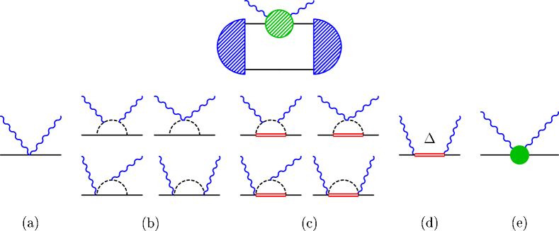
Figure 1: One-nucleon contributions to $\gamma d$ scattering in SSE $\chi$EFT at order $\epsilon^{3}$ (permuted and crossed diagrams not shown). Top: embedding into the deuteron. Bottom: one-nucleon Thomson term (a); pion cloud around the nucleon (b) and $\Delta(1232)$ (double line; (c)); excitation of an intermediate $\Delta$ (d); short-distance effects to $\alpha_{E1}$ and $\beta_{M1}$ (e).

1. Thomson scattering on one nucleon, Fig. 1 (a).

2. Coupling to the chiral dynamics of the pion cloud around one nucleon Fig. 1 (b).

3. Excitation of the $\Delta(1232)$ intermediate state, Fig. 1 (d), and coupling to the pion cloud around it Fig. 1 (c). The relevance of the $\Delta(1232)$ will be discussed in Sec. III.

4. Two energy-independent, iso-scalar short-distance coefficients, Fig. 1 (e). They encode the contributions to the nucleon polarisabilities which come at this order neither from the deformation of the pion cloud around the nucleon or $\Delta$, nor from the excitation of the $\Delta$ itself. Strictly speaking, they are formally of higher order, $\mathcal{O}({\epsilon}^{4})$. However, we follow Refs. Hi04 ; Hi05a ; Hi05b ; Hi05 in modifying the SSE to account for the stark discrepancy between the experimental static spin-independent dipole polarisabilities and the $\mathcal{O}({\epsilon}^{3})$ SSE values due to $\Delta$ effects. These “off-sets” are determined by data as described below, but the energy- and isospin-dependence of the spin-independent polarisabilities are at this order predicted in SSE $\chi$EFT.

5. Since the deuteron is an iso-scalar, there is no contribution from the iso-vector $t$-channel $\pi^{0}$ coupling to two photons via the axial anomaly.

Polarisabilities parameterise the “structure” part of the amplitudes and contain – as any multipole-expansion – not more or less information than the amplitude itself. However, decomposing into channels of different multipolarity makes the information more easily accessible and interpretable. For example, the strongly para-magnetic coupling of the photon and nucleon to the dynamical $\Delta$ dominates the energy-dependence of the polarisabilities $\beta_{M1}$ and $\gamma_{M1M1}$, while pion-cloud effects dominate $\alpha_{E1}$ and $\gamma_{E1E1}$. At this order in SSE, the polarisabilities are uniquely extracted from the sum of contributions 2 to 5, see Hi04 . While there is some ambiguity which makes it necessary to specify exactly how the “pole” and “structure” parts are divided, this artificial separation has of course no bearing on observables. We also found that contributions from quadrupole and higher polarisabilities are negligible in the present analysis, as was the case in unpolarised observables Hi04 ; Hi05b ; Hi05 .

The numerical values of all parameters were taken from Ref. (Hi05a, , Table 1). In particular, the strength of the $\gamma N\Delta$ vertex is determined by the decay $\Delta\rightarrow\gamma N$. In addition, the two short-distance contributions to the spin-independent polarisabilities are fitted to the 28 data of elastic deuteron Compton scattering below $100\;\mathrm{MeV}$, using the iso-scalar Baldin sum-rule

$$\alpha_{E1}+\beta_{M1}=14.5\pm 0.6$$ (6)

as constraint Olmos ; Ko03 . This value is within error-bars of a SAID analysis Ar02 and an extraction by Levchuk and L’vov Lv00 . The results of the static spin-independent polarisabilities are given in (2), Refs. Hi05 ; Hi05b . At this order in $\chi$EFT, the proton and neutron polarisabilities are identical, and the spin-polarisabilities are parameter-free predictions. For reference, the central values of the iso-scalar dipole polarisabilities are quoted from Hildebrandt et al. Hi04 ; Hi05 ; Hi05b (with theoretical uncertainties of $\approx\pm 1$ from higher-order contributions):

$${\alpha}_{E1}=11.3\;\; \;\;{\beta}_{M1}=3.2$$ ,

$$\gamma_{E1E1}=-5.5\;\;,\;\;\gamma_{M1M1}=3.1\;\; \;\;\gamma_{M1E2}=1.0\;\;,\;\;\gamma_{E1M2}=1.0$$ , (7)

There are two classes of diagrams in the two-nucleon sector, see Fig. 2, in extension of the $\chi$EFT $\mathcal{O}(Q^{3})$ amplitudes without explicit $\Delta(1232)$ which were derived for $\omega\sim m_{\pi}$ in Be99 :

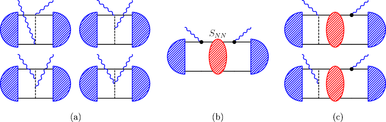
Figure 2: Two-nucleon contributions to $\gamma d$ scattering in SSE $\chi$EFT at order $\epsilon^{3}$ (permuted and crossed diagrams not shown). Photons couple to the same pion (a); re-scattering contributions ((b,c); ellipse: two-nucleon $S$-matrix; dot: coupling via minimal substitution or magnetic moment).

1. Both photons couple to the same pion-exchange current, Fig. 2 (a) Be99 .

2. Rescattering contributions, Fig. 2 (b/c): The photons couple to the nucleon charge, magnetic moment and/or to different pion-exchange currents. Between the two photon couplings, the nucleons re-scatter arbitrarily often, via the full $NN$ S-matrix. These parts are computed in the “Green’s Function Hybrid Approach” detailed in Refs. Hi05b ; Hi05 ; Ka99 and references therein.

One can show that the latter contribution must be included in any consistent power-counting of $\chi$EFT for the two-nucleon system Griesshammer:2007aq ; hgrieproc ; hgrieforthcoming . This can be understood intuitively as follows: The initial coherent two-nucleon state is not perturbed too much by absorbing or emitting a very-low-energy photon with energy $\omega$. Due to the large $NN$ scattering lengths, the two nucleons can interact multiple times over a typical time- and length-scale $1/\omega$ before another photon is emitted, producing a final state which contains an outgoing photon and a deuteron. It has been demonstrated by Friar and Arenhövel that these rescattering contributions ensure the correct Thomson limit of $\gamma d$ scattering. This exact low-energy theorem is a consequence of current conservation, which turn is equivalent to gauge-invariance at this order Friar ; We83 ; We83a . In contradistinction, rescattering contributions become small and hence perturbative at higher photon energies. This is intuitively clear, as the struck nucleon has then only a very short time $\sim 1/\omega$ to scatter with its partner before the coherent final state must be restored. Reference Hi05 ; Hi05b showed that rescattering contributions are negligible in unpolarised Compton scattering for $\omega\gtrsim 60\;\mathrm{MeV}$, except for a markedly suppressed residual dependence on the details of the deuteron wave function used. The importance of rescattering for polarisation observables will be assessed in Sec. III.

With the correct Thomson limit and explicit $\Delta$-degrees of freedom, the range of validity of SSE $\chi$EFT spans therefore in principle from $\omega=0$ to the the $\Delta$ resonance region, where finite $\Delta$-with effects must be taken into account. In practise, the present formulation puts the pion-production threshold $\gamma d\to\pi X$ not at the exact kinematically correct position, but higher orders in $\epsilon$ include the deuteron recoil effects in perturbation. Since the polarisabilities and observables around threshold are quite sensitive to the exact threshold position Hi05a ; Hi05 , we limit the discussion to $\omega\lesssim 120\;\mathrm{MeV}$, where such effects are small.

By convoluting phenomenological wave-functions with interactions from EFT, we follow a “hybrid approach” advocated by Weinberg Weinberg ; Weinberg2 . As in Hi05b ; Hi05 , the Argonne V18 potential AV18 is used to produce the $NN$-rescattering matrix, together with the “NNLO” $\chi$EFT deuteron wave-function at cut-off $650\;\mathrm{MeV}$ Epelbaum ; Epelbaum2 . Since the deuteron is an iso-scalar, neither the deuteron wave-function nor the intermediate $NN$ potential contains a $\Delta N$ component, so that using wave-functions and potentials without explicit $\Delta$ degrees of freedom is justified. We also verified that using instead the AV18 or Nijmegen93 Nijm93 deuteron wave-functions, or the LO chiral potential to generate the $NN$ S-matrix in the intermediate state, induces only negligible differences $\lesssim 3\%$ in all observables even at $\omega\approx 125\;\mathrm{MeV}$, as found for unpolarised cross-sections in Hi05 ; Hi05b . In a fully self-consistent EFT calculation, the kernel, wavefunctions and potential should of course be derived in the same framework. However, issues of matching electro-magnetic currents Kolling:2009iq ; Pastore:2009is , wave-functions and potentials only appear at two higher orders than considered here and may thus be taken as estimate of the size of higher-order corrections. At lower energies, the Thomson limit decreases this residual uncertainty even more, since Friar and Arenhövel demonstrated that for $\omega\to 0$, the Thomson limit is restored for any combination of potential and wave-function Friar ; We83 ; We83a . Numerically, the Thomson limit is fulfilled on the $0.6\%$-level.

We close by clearly stating the limitations of this analysis. The purpose is a study emphasising the relative sensitivity of Compton scattering observables on varying the polarisabilities. Credible predictions of their absolute magnitudes are however only meaningful when all systematic uncertainties are properly propagated into observables. Such errors include: theoretical uncertainties from discarding contributions in SSE $\chi$EFT which are higher than order $\epsilon^{3}$; uncertainties from data and the Baldin Sum rule in $\alpha_{E1}$ and $\beta_{M1}$ (2); and to a lesser extend error-bars of the $\gamma N\Delta$ determination, residual wave-function and potential dependence as well as numerical uncertainties. Such an effort is under way as part of a comprehensive approach of Compton scattering on the proton, deuteron and ³He in $\chi$EFT from zero energy to beyond the pion-production threshold allofus .

II.2 Observables

With 2 photon helicities $\lambda_{i/f}=\pm 1$ and 3 value for the deuteron polarisation $M_{i/f}\in\{0;\pm 1\}$ in both the in- and out-state, $(2\times 3)^{2}=36$ helicity amplitudes exist. As constructed by Chen, Ji and Li, parity and time-reversal symmetry leave 12 independent structures describing scattering of photons on a spin-$1$ target. A scalar or umpolarised target probes $2$ of them, a vector-polarised one $4$, and a tensor-polarised $6$. As each amplitude is complex and the overall phase is fixed, $23$ independent observables per energy and angle are needed to fully determine the Compton scattering amplitude. Our goal is however not a comprehensive study of all observables with polarised in and/or out states. Rather, we only consider elastic reactions in which the polarisations in the final state are not detected and the initial deuteron is either unpolarised or vector-polarised. Amongst these, several are not independent. We look for those with the strongest signal of scalar and spin-polarisabilities.

We define our co-ordinate system by choosing the beam direction to be the $z$-axis, the scattering plane to be the $xz$-plane, with the $y$-axis perpendicular to it. The differential cross-section for unpolarised deuteron Compton scattering is

$$\frac{\mathrm{d}\sigma}{\mathrm{d}\Omega}=\Phi^{2}\frac{1}{6}\sum\limits_{M_{f},M_{i};\lambda_{f},\lambda_{i}}|\mathcal{M}_{\lambda_{f},\lambda_{i}}^{M_{f},M_{i}}|^{2}\;\;.$$ (8)

The factor $\frac{1}{6}$ comes from averaging over the initial deuteron and photon polarisations. In the centre-of-mass (cm) and laboratory (lab) frames, the phase-space factor $\Phi$ is:

$$\Phi_{\rm cm} = \dfrac{M_{d}}{4\pi\sqrt{s_{\gamma d}}}\;\;,\;\;\mbox{ where }\,s_{\gamma d}=\omega+\sqrt{\omega^{2}+M_{d}^{2}}$$

$$\Phi_{\rm lab} = \dfrac{\omega_{f}}{4\pi\omega_{i}}\;\;,\;\;\mbox{ where }\,\,\omega_{f}=\dfrac{M_{d}\omega_{i}}{M_{d}+\omega_{i}(1-\cos\theta_{\rm lab})}\;\;.$$ (9)

Here, $\theta_{\text{lab}}$ is the scattering angle in the lab frame, $M_{d}$ the deuteron mass, $\omega_{i}$ ($\omega_{f}$) the initial (final) photon energy in the lab frame, $\sqrt{s_{\gamma d}}$ the total energy in the $\gamma d$ cm frame, and $\omega=\frac{\omega_{i}}{\sqrt{1+2\omega_{i}/M_{d}}}$ the photon energy in the cm frame.

A host of observables can be defined in deuteron Compton scattering with incoming circularly or linearly polarised photon beams and unpolarised or polarised deuteron targets, but without detection of the final-state polarisations. We consider here only subset involving an unpolarised or vector-polarised deuteron.

Two independent observables exist for linearly-polarised photons and an unpolarised target, Fig. 3.

Figure 3: (Colour online) Observables for incoming linearly-polarised photon and unpolarised target.

The cross-section for an incoming photon polarised in the scattering plane is denoted by $\left[\dfrac{\mathrm{d}\sigma}{\mathrm{d}\Omega}\right]^{\text{lin}}_{x}$, and by $\left[\dfrac{\mathrm{d}\sigma}{\mathrm{d}\Omega}\right]^{\text{lin}}_{z}$ for polarisation perpendicular to the scattering plane:

$$\left[\dfrac{\mathrm{d}\sigma}{\mathrm{d}\Omega}\right]^{\text{lin}}_{x} = \dfrac{\Phi^{2}}{3}\sum\limits_{M_{f},M_{i};\lambda_{f},\lambda_{i}=\hat{x}}|\mathcal{M}_{\lambda_{f}}^{M_{f},M_{i}}|^{2}$$ (10)

$$\left[\dfrac{\mathrm{d}\sigma}{\mathrm{d}\Omega}\right]^{\text{lin}}_{y} = \dfrac{\Phi^{2}}{3}\sum\limits_{M_{f},M_{i};\lambda_{f},\lambda_{i}=\hat{y}}|{\mathcal{M}}_{\lambda_{f}}^{M_{f},M_{i}}|^{2}.$$ (11)

It was already shown in Ref. Ch05 that the corresponding photon polarisation asymmetry

$$\Pi^{\text{lin}}=\left(\left[\dfrac{\mathrm{d}\sigma}{\mathrm{d}\Omega}\right]^{\text{lin}}_{x}-\left[\dfrac{\mathrm{d}\sigma}{\mathrm{d}\Omega}\right]^{\text{lin}}_{y}\right)/\dfrac{\mathrm{d}\sigma}{\mathrm{d}\Omega}$$ (12)

is not a good observable to extract the polarisabilities.

There are four observables for which both beam and target are polarised.

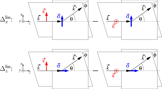
Figure 4: (Colour online) Observables for linearly-polarised photon on vector-polarised target.

The double-polarisation observables with linearly polarised photons $\left(\lambda_{i}\in\left\{\hat{x},\hat{y}\right\}\right)$ are shown in Fig. 4. One is the cross-section difference on a target polarised in a plane perpendicular to the beam direction and target polarisations parallel vs. perpendicular to that of the incoming photon:

$$\Delta_{x}^{\text{lin}}=\left(\frac{\mathrm{d}\sigma}{\mathrm{d}\Omega}\right)_{\hat{x}\rightarrow}-\left(\frac{\mathrm{d}\sigma}{\mathrm{d}\Omega}\right)_{\hat{y}\rightarrow}$$ (13)

The subscripts $\hat{x}$ or $\hat{y}$ describe the initial photon polarisation, and the arrows denote the initial target polarisation ($\uparrow\equiv+\hat{z}$ and $\rightarrow\equiv+\hat{x}$). The other observable measures the same photon polarisation differences on a target polarised along the beam direction:

$$\Delta_{z}^{\text{lin}}=\left(\frac{\mathrm{d}\sigma}{\mathrm{d}\Omega}\right)_{\hat{x}\uparrow}-\left(\frac{\mathrm{d}\sigma}{\mathrm{d}\Omega}\right)_{\hat{y}\uparrow}$$ (14)

Both observables depend also on the angle $\phi$ between the scattering plane and the plane formed by beam direction and the incoming photon polarisation. The best signals are found when both planes coincide, $\phi=0$.

The double-polarisation observables with circularly polarised photons $\lambda_{i}=\mp\dfrac{\hat{x}+i\hat{y}}{\sqrt{2}}$, with $\lambda_{i}=\pm 1$ for photons with positive or negative helicity, are shown in Fig. 5.

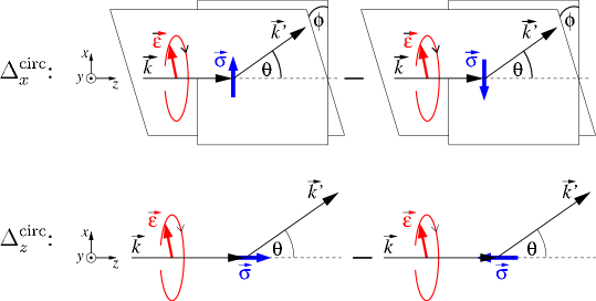
Figure 5: (Colour online) Observables for circularly-polarised photon on vector-polarised target.

The deuteron target can again be vector-polarised in the scattering plane along $\hat{x}$ or along the beam-direction $\hat{z}$. Cross-section differences are found by flipping the target polarisation. For any incoming photon helicity:

$$\Delta_{x,(\lambda_{i}=\pm 1)}^{\text{circ}} = \left(\frac{\mathrm{d}\sigma}{\mathrm{d}\Omega}\right)_{\uparrow\rightarrow}-\left(\frac{\mathrm{d}\sigma}{\mathrm{d}\Omega}\right)_{\uparrow\leftarrow}$$ (15)

$$\Delta_{z,(\lambda_{i}=\pm 1)}^{\text{circ}} = \left(\frac{\mathrm{d}\sigma}{\mathrm{d}\Omega}\right)_{\uparrow\uparrow}-\left(\frac{\mathrm{d}\sigma}{\mathrm{d}\Omega}\right)_{\uparrow\downarrow}$$ (16)

The first arrow of the subscript denotes the beam helicity; the second the target polarisation. The perpendicular polarisation $\Delta_{x}^{\text{circ}}$ is the difference of the differential cross-sections with the target polarised along $+\hat{x}$ vs. $-\hat{x}$, i.e. perpendicular to the beam helicity. It depends again on the angle $\phi$ between the polarisation and scattering planes, with best results for $\phi=0$. Similarly, the parallel polarisation $\Delta_{z}^{\text{circ}}$ is the difference with target polarised parallel vs. anti-parallel to the beam helicity and is independent of $\phi$. In Ref. Chen:2004wwa , the same quantity is denoted by $2\Delta_{1}\sigma$.

Of the four quantities $\Delta^{\text{lin/circ}}_{x/z}$, only two are linearly independent, namely for example those which involve circularly polarised photons, or alternatively linearly polarised photons. We look for those with the strongest polarisability signal.

The cross-section differences $\Delta$ set the scale for count-rates, and hence for the beamtime necessary. Normalising to sums of cross-sections removes many systematical experimental uncertainties. As pointed out in Ch05 , the denominators are not total unpolarised cross-sections since one deals with a spin-$1$ target. The polarisation asymmetries $\Sigma$ are :

$$\Sigma_{x}^{\text{lin}} = \frac{\left(\frac{\mathrm{d}\sigma}{\mathrm{d}\Omega}\right)_{\hat{x}\rightarrow}-\left(\frac{\mathrm{d}\sigma}{\mathrm{d}\Omega}\right)_{\hat{y}\rightarrow}}{\left(\frac{\mathrm{d}\sigma}{\mathrm{d}\Omega}\right)_{\hat{x}\rightarrow}+\left(\frac{\mathrm{d}\sigma}{\mathrm{d}\Omega}\right)_{\hat{y}\rightarrow}}$$ (17)

$$\Sigma_{z}^{\text{lin}} = \frac{\left(\frac{\mathrm{d}\sigma}{\mathrm{d}\Omega}\right)_{\hat{x}\uparrow}-\left(\frac{\mathrm{d}\sigma}{\mathrm{d}\Omega}\right)_{\hat{y}\uparrow}}{\left(\frac{\mathrm{d}\sigma}{\mathrm{d}\Omega}\right)_{\hat{x}\uparrow}+\left(\frac{\mathrm{d}\sigma}{\mathrm{d}\Omega}\right)_{\hat{y}\uparrow}}$$ (18)

$$\Sigma_{z,(\lambda_{i}=\pm 1)}^{\text{circ}} = \frac{\left(\frac{\mathrm{d}\sigma}{\mathrm{d}\Omega}\right)_{\uparrow\uparrow}-\left(\frac{\mathrm{d}\sigma}{\mathrm{d}\Omega}\right)_{\uparrow\downarrow}}{\left(\frac{\mathrm{d}\sigma}{\mathrm{d}\Omega}\right)_{\uparrow\uparrow}+\left(\frac{\mathrm{d}\sigma}{\mathrm{d}\Omega}\right)_{\uparrow\downarrow}}$$ (19)

$$\Sigma_{x,(\lambda_{i}=\pm 1)}^{\text{circ}} = \frac{\left(\frac{\mathrm{d}\sigma}{\mathrm{d}\Omega}\right)_{\uparrow\rightarrow}-\left(\frac{\mathrm{d}\sigma}{\mathrm{d}\Omega}\right)_{\uparrow\leftarrow}}{\left(\frac{\mathrm{d}\sigma}{\mathrm{d}\Omega}\right)_{\uparrow\rightarrow}+\left(\frac{\mathrm{d}\sigma}{\mathrm{d}\Omega}\right)_{\uparrow\leftarrow}}$$ (20)

Nevertheless, division by a small spin-averaged cross-section may enhance theoretical uncertainties, or hide un-feasibly small count-rates. We also find that asymmetries $\Sigma$ are usually by $\lesssim 30$% less sensitive to variations of the polarisabilities than cross-section differences $\Delta$. Sometimes, sensitivity to the nucleon structure is even lost entirely, while in no case do we see an enhancement. It is the purview of our experimental colleagues to determine whether these draw-backs outweigh the benefits.

II.3 Strategy

In analysing the sensitivity of a given polarisation observable on the dipole polarisabilities, we adopt the approach of Ref. Ch05 to vary the static central values as given in eq. (7) by adding one energy-independent parameter for each dipole polarisability, labelled $\delta\alpha_{E1}$, $\delta\beta_{M1}$, $\delta\gamma_{E1E1}$, $\delta\gamma_{M1M1}$, $\delta\gamma_{E1M2}$ and $\delta\gamma_{M1E2}$. In the notation and definition of dynamical polarisabilities of Ref. Hi04 , but without a kinematical prefactor $(\omega+\sqrt{\omega^{2}+M^{2}})/M$, the complete $\mathcal{O}(\epsilon^{3})$ one-nucleon amplitudes of Sec. II.1 in the cm frame of the $\gamma N$ system are thus supplemented by

$${A}^{\mathrm{fit}}(\omega,\,z) = 4\pi\,\omega^{2}\,\bigg{[}[\delta\alpha_{E1}+z\,\delta\beta_{M1}]\,(\vec{\epsilon}^{\prime}\cdot\vec{\epsilon})-\delta\beta_{M1}\,(\vec{\epsilon}^{\prime}\cdot\hat{k})\,(\vec{\epsilon}\cdot\hat{k}^{\prime})$$ (21)

$$-\mathrm{i}\,[\delta\gamma_{E1E1}+z\,\delta\gamma_{M1M1}+\delta\gamma_{E1M2}+z\,\delta\gamma_{M1E2}]\,\omega\,\vec{\sigma}\cdot(\vec{\epsilon}^{\prime}\times\vec{\epsilon})$$

$$+\mathrm{i}\,[\delta\gamma_{M1E2}-\delta\gamma_{M1M1}]\,\omega\,\vec{\sigma}\cdot\left(\hat{k}^{\prime}\times\hat{k}\right)(\vec{\epsilon}^{\prime}\cdot\vec{\epsilon})$$

$$+\mathrm{i}\,\delta\gamma_{M1M1}\,\omega\,\vec{\sigma}\cdot\left[\left(\vec{\epsilon}^{\prime}\times\hat{k}\right)(\vec{\epsilon}\cdot\hat{k}^{\prime})-\left(\vec{\epsilon}\times\hat{k}^{\prime}\right)(\vec{\epsilon}^{\prime}\cdot\hat{k})\right]$$

$$+\mathrm{i}\,\delta\gamma_{E1M2}\,\omega\,\vec{\sigma}\cdot\left[\left(\vec{\epsilon}^{\prime}\times\hat{k}^{\prime}\right)(\vec{\epsilon}\cdot\hat{k}^{\prime})-\left(\vec{\epsilon}\times\hat{k}\right)(\vec{\epsilon}^{\prime}\cdot\hat{k})\right]\bigg{]}\;\;.$$

The full amplitudes are then embedded into the deuteron as extension of diagram (e) in Fig. 1. Here, $\vec{\epsilon}$ and $\hat{k}$ ($\vec{\epsilon}^{\prime}$ and $\hat{k}^{\prime}$) are the polarisation and direction of the incoming (outgoing) photon in the $\gamma N$ cm frame, and $z=\hat{k}\cdot\hat{k}^{\prime}$. Except for the kinematically convenient pre-factor $\sqrt{s_{\gamma N}}/M$, this form is identical to that derived from the interaction (1).

One can think of these contributions as parameterising the difference between predicted and (so-far un-measured) experimental static values of the polarisabilities, under the assumption that the energy-dependence of the dipole polarisabilities is predicted correctly in SSE $\chi$EFT. Conceptually, this would imply that these additional interactions parameterise energy-independent, short-distance contributions to the amplitudes, i.e. contributions which are at this order not explained by pion-cloud or $\Delta$ effects. Alternatively, one can also see them as parameterising deviations from the SSE $\chi$EFT amplitudes at fixed nonzero energy, including the theoretical uncertainties of higher-order effects. In that case, the deviations themselves could be seen as energy-dependent. To reiterate, this analysis is only sensitive to the average proton and neutron dipole polarisabilities, since the deuteron is an iso-scalar.

In the next step, these contributions are independently varied by $\pm 2$ canonical units for one nucleon to analyse the effect of each on the various observables. The polarisabilities of the other nucleon are kept fixed at the iso-scalar value. This corresponds to a change of the iso-scalar polarisabilities by half as much, i.e. by $\pm 1$ unit. Since deuteron Compton scattering is sensitive only to iso-scalar quantities, varying either the proton or neutron polarisabilities leads to the same result. In practise, the scalar polarisabilities of the proton are better constrained, and deuteron Compton scattering experiments are more likely focused on extracting neutron polarisabilities. In that case, these studies can be interpreted as providing the sensitivities on varying the neutron polarisabilities by $\pm 2$ units, with fixed proton polarisabilities. The spin-independent polarisabilities are known to better accuracy, see eq. (2). But the goal is to compare their sensitivity to those of the much less accurately known spin-polarisabilities, for which different theoretical descriptions can disagree by as much as $4$ units, see discussion below (3) and (4). We therefore see a variation of $\pm 2$ units as a compromise and note that variation by other amounts is easily obtained from the one given since all observables are linear in the variations $\delta(\alpha,\beta,\gamma_{i})$. Quadratic contributions in the variations contribute $\lesssim 1\%$ to observables.

As hinted above, the polarisabilities are the multipoles of the structure part of the amplitudes and thus do not contain more or less information than the corresponding amplitudes. Therefore, determining the dipole polarisabilities is now in principle reduced to a multipole-analysis of $6+1$ high-accuracy scattering experiments using (21), as outlined in hgrieproc ; Miskimentalk .

However, we do not present the result of the analysis in its entirety here. Additional constraints must be considered in real life. The sum of electric and magnetic polarisabilities is related by the Baldin sum rule (6), and weaker constraints exist from the forward and backward spin-polarisabilities (3/4). Experimental constraints like detector and polarisation efficiencies and existing deuteron Compton scattering data must be taken into account, too, to determine which experiments will indeed show the greatest sensitivity on a given polarisability and have the greatest impact in the network of data already available.

Cross-section differences $\Delta$ and asymmetries $\Sigma$ for $6$ observables, depending on $6$ dipole polarisabilities and $3$ kinematic variables (photon energy $\omega$ and scattering angles $\theta$ and $\phi$) in the cm and lab frame, plus additional constraints, provide a large number of parameters to explore. Since the full information can not adequately be conveyed in an article, we focus only on some prominent examples here and note that in order to aide in planning and analysing experiments, the results for all observables are available as an interactive Mathematica 7.0 notebook from Grießhammer (hgrie@gwu.edu). It contains both tables and plots of energy- and angle-dependences of the cross-sections, cross-section differences, analysing powers and asymmetries from $10$ to about $120$ MeV, in both the cm and lab systems, including sensitivities to varying the spin-independent and spin-dependent polarisabilities independently and subject to the Baldin sum rule constraint (6). Figure 6 shows a sample screen-shot.

Figure 6: (Colour online) Screen-shot of part of the interactive Mathematica notebook.

In this article, we therefore focus on two representative energies in the lab-frame as the one which is experimentally most relevant. At $\omega_{\text{lab}}=45\;\mathrm{MeV}$, spin-polarisabilities should be suppressed since they scale as $\omega^{3}$, see eq. (21), while spin-independent polarisabilities are already noticeable since they scale as $\omega^{2}$. On the other hand, spin-polarisabilities should provide a substantial contribution at $\omega_{\text{lab}}=125\;\mathrm{MeV}$, while staying below the pion-production threshold avoids experimental and theoretical complications.

III Significance of $\Delta$-Isobar and $NN$-Rescattering

We now analyse the effect of the $\Delta$-isobar and intermediate $NN$-rescattering contributions on polarisation observables. Without explicit $\Delta$, the ingredients are that of Heavy-Baryon $\chi$EFT at order $Q^{3}$, where Q is again a typical small momentum scale, now measured in units of the breakdown scale ${\mathrm{Re}}[M_{\Delta}]-M\approx 300\;\mathrm{MeV}$ of the $\Delta$-less theory. Results with and without explicit $\Delta$ compare HB$\chi$EFT power-counting scheme at $\mathcal{O}(Q^{3})$ with that of SSE at $\mathcal{O}(\epsilon^{3})$. The latter is a more accurate description at higher energies due to its larger radius of convergence. Since effects from the dynamical $\Delta$ are small at low energies, both results should agree inside the radius of convergence of HB$\chi$EFT. By comparing HB$\chi$EFT and SSE, one can thus judge where HB$\chi$EFT does not converge any more.

On the other hand, leaving out $NN$-rescattering contributions is justified in an order-by-order expansion of the amplitudes only for high photon energies, $\omega\sim m_{\pi}$ Be04 ; Griesshammer:2007aq ; hgrieforthcoming . As discussed in Sec. II.1, rescattering is mandatory in any consistent power-counting at lower energies to restore the deuteron Thomson limit Griesshammer:2007aq ; hgrieforthcoming . Without it, the calculation is inconsistent at low energies. At higher energies, the theory remains perturbatively consistent since rescattering introduces then by design a large number of two-body amplitudes which are formally of higher order Be04 ; Hi05 ; Hi05b ; Griesshammer:2007aq . The approaches with and without rescattering should thus coincide for high enough energies. Their comparison provides thus a tool to estimate a low-energy limit for expanding the rescattering amplitude.

In unpolarised Compton scattering, Refs. Hi05 ; Hi05a showed that even though ${\mathrm{Re}}[M_{\Delta}]-M\approx 300$ MeV, the $\Delta(1232)$ provides considerable strength at much lower energies ($\approx 100\;\mathrm{MeV}$), due to its strong paramagnetism. This modifies the energy-dependent polarisabilities $\beta_{M1}$ and $\gamma_{M1M1}$ dramatically and resolved the “SAL Puzzle” Ka99 ; Lv00 ; Hornidge ; Levchuk:2000mg ; Be99 ; Be04 of the apparent disagreement of both predictions and post-dictions with data around $100\;\mathrm{MeV}$ at backward angles Hi05a ; Hi05 ; Hi05b . In contrast, including $NN$-rescattering in the intermediate state proved essential only for $\omega\sim\frac{m_{\pi}^{2}}{M}\lesssim 50\;\mathrm{MeV}$, while rescattering contributions provided only perturbative corrections at $\omega_{\text{lab}}\gtrsim 80\;\mathrm{MeV}$ Hi05 ; Hi05a ; Hi05b .

Turning to polarisation observables, Figs. 7 and 8

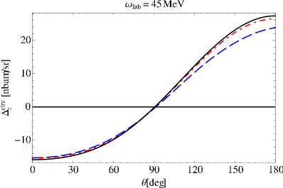
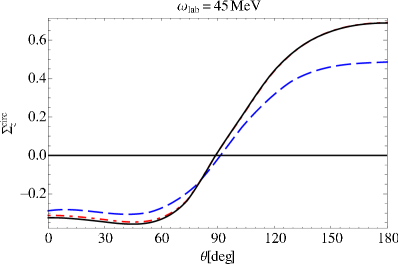
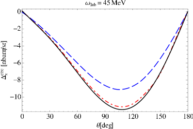
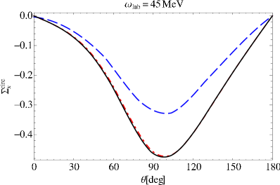
Figure 7: (Colour online) Dependence of typical polarisation observables at $\omega_{\text{lab}}=45$ MeV on rescattering and $\Delta$-effects. Left: $\Delta_{z}^{\text{circ}}$ (upper) and $\Delta_{x}^{\text{circ}}$ (lower); right: corresponding asymmetries $\Sigma_{z}$ and $\Sigma_{x}$. Dashed (blue): $\mathcal{O}(Q^{3})$ HB$\chi$EFT without rescattering (no $\Delta$); dot-dashed (red): complete $\mathcal{O}(Q^{3})$ (with $NN$-rescattering, no $\Delta$); solid (black): full $\mathcal{O}(\epsilon^{3})$ (with $\Delta$ and $NN$-rescattering).

show cross-section differences $\Delta^{\text{circ}}_{x,z}$ and asymmetries $\Sigma^{\text{circ}}_{x,z}$ with circularly-polarised photons in the lab frame at $\omega_{\text{lab}}=45\;\mathrm{MeV}$ and $\omega_{\text{lab}}=125\;\mathrm{MeV}$, respectively, with and without including the contributions from $NN$-rescattering or from a dynamical $\Delta$. The other observables show a similar behaviour.

In scattering at $45\;\mathrm{MeV}$, Fig. 7, effects from rescattering are substantial. The dashed (blue) lines neither include rescattering nor a dynamical $\Delta$, while the dot-dashed (red) lines include rescattering and thus provide a consistent $\mathcal{O}(Q^{3})$ HB$\chi$EFT calculation (no $\Delta$). By comparing the latter with the consistent $\mathcal{O}(\epsilon^{3})$ SSE result, solid (black) line, one concludes that a dynamical inclusion of the $\Delta$ is not necessary at this energy. In asymmetries (right panels), rescattering is slightly more pronounced than in cross-section differences (left panels). Within theoretical uncertainties, $\Delta$-effects are the same in both.

As expected, $\Delta$-effects have become pronounced at $125\;\mathrm{MeV}$, see Fig. 8.

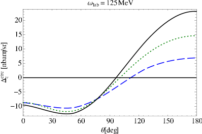
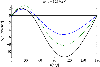
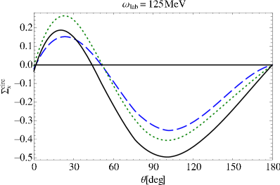
Figure 8: (Colour online) Dependence of typical polarisation observables at $\omega_{\text{lab}}=125$ MeV on rescattering and $\Delta$-effects. Left: $\Delta_{z}^{\text{circ}}$ (upper) and $\Delta_{x}^{\text{circ}}$ (lower); right: the corresponding asymmetries $\Sigma_{z}$ and $\Sigma_{x}$. Dashed (blue): $\mathcal{O}(Q^{3})$ HB$\chi$EFT without rescattering (no $\Delta$); dotted (green): $\mathcal{O}(\epsilon^{3})$ (with $\Delta$) but no $NN$-rescattering; solid (black): full $\mathcal{O}(\epsilon^{3})$ (with $\Delta$ and $NN$-rescattering).

A dynamical $\Delta$ without rescattering (dotted green) nearly doubles $\Delta^{\text{circ}}_{x,z}$, compared to the HB$\chi$EFT result without rescattering (dashed blue). Surprisingly and in contradistinction to unpolarised observables, rescattering effects provide an additional sizable correction of up to $40\%$ in SSE (solid black). In asymmetries (right panels), both effects are usually slightly smaller. The large rescattering correction suggests that contributions in which the photons couple to the same pion-exchange current, Fig. 2 (a), are not as prominent in the polarisation observables as in unpolarised ones. For single-polarisation observables, Ref. mythesis ; Ch05 pointed already out that this can be attributed to the near-diagonal spin-structure of the two-body currents. Clearly, the intermediate $NN$ rescattering matrix is highly off-diagonal in angular-momentum space due to the electric and magnetic couplings and photon multipolarity. Since rescattering should at these energies be perturbative as discussed in Sect. II.1, truncating the expansion at lowest order, i.e. with only one intermediate pion exchange as performed in Ref. Be02 ; Be04 may suffice to obtain the same result. According to the power-counting in that régime, such contributions are of higher order. This raises the question to which extend the $\chi$EFT expansion converges. Only typical sizes of contributions are however estimated by power-counting. A comprehensive answer can only be given a complete next-order calculation in $\chi$EFT.

Thus, both the dynamical $\Delta$-isobar and intermediate $NN$-rescattering contributions are necessary in polarisation observables up to $125$ MeV. The latter is a remnant of the Thomson limit even at high energies. The former must be included since the $\gamma\Delta N$ coupling induces large paramagnetic effects whose energy-dependence is crucial at high energies. At low energies, however, the $\Delta$ is indeed and as expected not dynamical. Both effects increase the magnitude of the asymmetry at back-angles for high energies, relative to a previous investigation Ch05 . In the following, we present only the complete SSE results, i.e. with dynamical $\Delta$ and $NN$-rescattering.

IV Unpolarised Target and Linearly-polarised Photons

Experiments with linearly polarised photons and unpolarised target, as planned or conducted at HI$\gamma$S Weller:2009zza ; Weller , are not only more readily realised than doubly-polarised experiments. They also provide an opportunity to consider kinematics in which at least one of the dipole polarisabilities does not contribute at all, facilitating extractions of the other ones.

While none of the observables described in Sec. II.2 is sensitive only to one dipole polarisability, inspecting (1) reveals configurations in which some polarisabilities do not contribute to Compton scattering, as to our knowledge first pointed out by Maximon for the proton Maximon:1989zz . Note that (1) involves double and triple scalar products between the electric and magnetic photon fields and the nucleon spin. First, re-write the electric spin-independent dipole term in (1) as $2\pi\alpha_{E1}(\omega)\;N^{\dagger}\,\vec{E}_{\text{in}}\cdot\vec{E}_{\text{out}}\,N$, where $\vec{E}_{\text{in}}$ ($\vec{E}_{\text{out}}$) is the electric field of the incoming (scattered) photon. There is no contribution when incoming and outgoing polarisations are orthogonal to each other. In the cm frame, this is the situation when the incoming photon polarisation is in the scattering plane and $\theta_{\text{cm}}=90^{\circ}$, see Fig. 9.

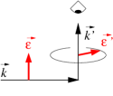
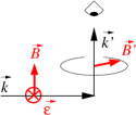
Figure 9: Left: Configuration under which an induced dipole cannot radiate an $E1$ photon into a detector; right: same for radiation of an $M1$ photon. The “eye” represents an observer.

Comparing to Fig. 3, $\left[\frac{\mathrm{d}\sigma}{\mathrm{d}\Omega}\right]^{\text{lin}}_{x}(\theta_{\text{cm}}=90^{\circ})$ is thus insensitive to $\alpha_{E1}$ when the photon is scattered off a nucleon. More intuitively, the induced time-dependent electric dipole moment $\vec{d}_{\text{ind}}=\alpha_{E1}\;\vec{E}_{\text{in}}$ in the nucleon leads to radiation from a Hertz’ian dipole, which emits no radiation along its axis.

Analogously, $\left[\frac{\mathrm{d}\sigma}{\mathrm{d}\Omega}\right]^{\text{lin}}_{y}(\theta_{\text{cm}}=90^{\circ})$ on a nucleon is insensitive to $\beta_{M1}$ because the induced magnetic dipole does not radiate under that angle, see Fig. 9. Similar arguments apply to the sensitivity of double-polarisation observables on spin-polarisabilities, see Sec. V.1.

For Compton scattering on the deuteron, the relative motion of the $\gamma N$ cm system must be taken into account. As the two nucleons are in a relative $S$ or $D$ wave in the deuteron, the conclusions remain unchanged, see Figs. 10 to 13.

Such arguments can of course be turned around: At $\theta_{\text{cm}}=90^{\circ}$, $\left[\frac{\mathrm{d}\sigma}{\mathrm{d}\Omega}\right]^{\text{lin}}_{x}$ should be most sensitive to $\beta_{M1}$, and $\left[\frac{\mathrm{d}\sigma}{\mathrm{d}\Omega}\right]^{\text{lin}}_{y}(\theta_{\text{cm}}=90^{\circ})$ to $\alpha_{E1}$, etc. However, embedding the nucleon into the deuteron changes these predictions. For example, the greatest sensitivity to $\beta_{M1}$ is for $\left[\frac{\mathrm{d}\sigma}{\mathrm{d}\Omega}\right]^{\text{lin}}_{x}$ actually found at $\theta\to 180^{\circ}$, see Fig. 10.

Turning first to the initial photon polarised in the scattering plane, i.e. to $\left[\frac{\mathrm{d}\sigma}{\mathrm{d}\Omega}\right]_{x}^{\text{lin}}$ (10), we consider the two energies $\omega_{\text{lab}}=$45 MeV and 125 MeV. In Fig. 10, the spin-independent polarisabilities are varied independently by $\pm 2$ units around the SSE values (7).

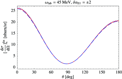
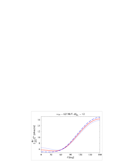
Figure 10: (Colour online) Dependence of $\left[\frac{\mathrm{d}\sigma}{\mathrm{d}\Omega}\right]^{\text{lin}}_{x}$ on the spin-independent dipole polarisabilities at $\omega_{\text{lab}}=45$ MeV (top) and $\omega_{\text{lab}}=125$ MeV (bottom) around the complete $\mathcal{O}(\epsilon^{3})$ calculation (solid red line). Left: $\alpha_{E1}$ varied by $\delta\alpha_{E1}=+2$ (dashed blue line); $\delta\alpha_{E1}=-2$ (dotted blue line). Right: Same for $\beta_{M1}$. Notice the scale offset in the lower panels.

The effect at 45 MeV does not exceed $\pm 0.2\;\mathrm{nbarn/sr}$, even at both forward and back angles where the sensitivity is most noticeable. At 125 MeV, there is with $\pm 0.4$ nbarn/sr limited but anti-correlated sensitivity to both $\alpha_{E1}$ and $\beta_{M1}$. As predicted above, $\left[\frac{\mathrm{d}\sigma}{\mathrm{d}\Omega}\right]_{x}^{\text{lin}}$ is indeed insensitive to $\alpha_{E1}$ at $\theta_{\text{cm}}=90^{\circ}$, i.e. $\theta_{\text{lab}}=88.65^{\circ}$ at $\omega_{\text{lab}}=45$ MeV and $86.41^{\circ}$ at $125$ MeV. At 45 MeV, a variation of the spin polarisabilities by $\pm$2 induces negligible effects ($\lesssim\pm 0.02$ nbarn/sr) and hence is not shown. This is expected because the spin-polarisabilities appear at higher order in energy than $\alpha_{E1}$ and $\beta_{M1}$. Figure 11 reports the sensitivity on varying the spin-polarisabilities one by one by $\pm$2 at $\omega_{\text{lab}}=125$ MeV.

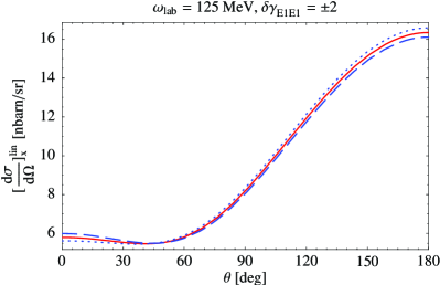
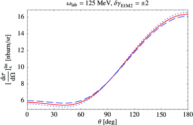
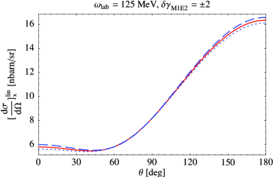
Figure 11: (Colour online) Dependence of $\left[\frac{\mathrm{d}\sigma}{\mathrm{d}\Omega}\right]^{\text{lin}}_{x}$ on the dipole spin-polarisabilities at $\omega_{\text{lab}}=125$ MeV around the complete $\mathcal{O}(\epsilon^{3})$ calculation. Variation of $\delta\gamma_{E1E1}=\pm 2$ (top left); $\delta\gamma_{M1M1}=\pm 2$ (top right); $\delta\gamma_{E1M2}=\pm 2$ (bottom left); $\delta\gamma_{M1E2}=\pm 2$ (bottom right). Notation as in Fig. 10. Notice the scale offset.

Although visible, this causes a maximum change of $\pm 0.25$ nbarn/sr. Note that $\gamma_{M1E2}$ does not contribute at $\theta_{\text{cm}}=90^{\circ}$. That there is neither dependence on $\gamma_{E1E1}$ at $\theta_{\text{lab}}\approx 45^{\circ}$ nor on $\gamma_{E1M2}$ at $\theta_{\text{lab}}\approx 90^{\circ}$, seems to be a fortunate accident, un-related to intuitive arguments like those above. A simultaneous experiment at various angles can thus dis-entangle individual spin-polarisabilities, with some of the experimental systematics cancelling. However, the small variations may make clear signals difficult to obtain.

Figure 12 shows plots analogous to Fig. 10 when the initial photons are polarised perpendicular to the scattering plane, i.e. for $\left[\frac{\mathrm{d}\sigma}{\mathrm{d}\Omega}\right]_{y}^{\text{lin}}$ (11)).

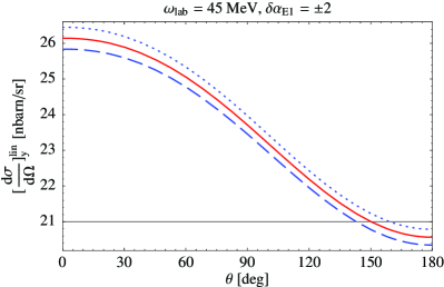
Figure 12: (Colour online) Dependence of $\left[\frac{\mathrm{d}\sigma}{\mathrm{d}\Omega}\right]^{\text{lin}}_{y}$ on the spin-independent dipole polarisabilities at $\omega_{\text{lab}}=45$ MeV (top) and $\omega_{\text{lab}}=125$ MeV (bottom). Notation as in Fig. 10. Notice the scale offset.

At 45 MeV, varying $\alpha_{E1}$ or $\beta_{M1}$ by $\pm$2 induces an effect of $\approx\pm$0.4 nbarn/sr effect, while the maximum sensitivity at 125 MeV is increased to $\approx\pm$0.7 nbarn/sr. Sensitivity to $\alpha_{E1}$ is quite uniform at all angles, while that to $\beta_{M1}$ vanishes at $\theta_{\text{cm}}=90^{\circ}$, as predicted.

A simultaneous extraction of both the electric and magnetic polarisabilities may thus be possible from the same observable. Particularly promising is measuring $\left[\frac{\mathrm{d}\sigma}{\mathrm{d}\Omega}\right]^{\text{lin}}_{y}(\theta_{\text{cm}}=90^{\circ})$, which gives $\alpha_{E1}$ and can be used as an input for the extraction of $\beta_{M1}$ from the same observable at other angles. Alternatively, one may use the same detector configuration $\theta_{\text{cm}}=90^{\circ}$ but change the linear beam polarisation from in-scattering-plane (insensitive to $\alpha_{E1}$) to perpendicular-to-scattering-plane (insensitive to $\beta_{M1}$), taking advantage of the cancellation of some systematic experimental uncertainties Weller .

Analogously to Fig. 11, we also present the same observable at $\omega_{\text{lab}}=$125 MeV in Fig. 13 when the spin polarisabilities are varied.

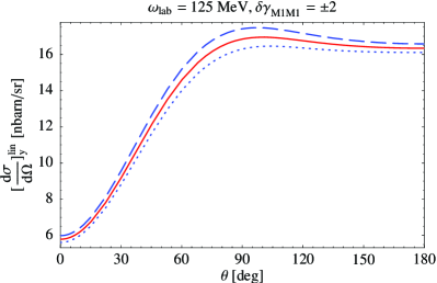
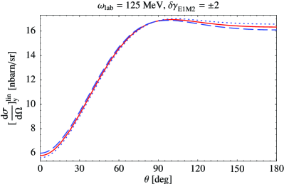
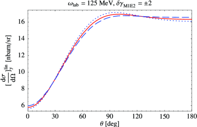
Figure 13: (Colour online) Dependence of $\left[\frac{\mathrm{d}\sigma}{\mathrm{d}\Omega}\right]^{\text{lin}}_{y}$ at $\omega_{\text{lab}}=125$ MeV on the dipole spin-polarisabilities. Notation as in Figs. 10 and 11. Notice the scale offset.

The maximum sensitivity of $\approx\pm$0.7 nbarn/sr is to $\gamma_{M1M1}$ around $90^{\circ}$, comparable to that on $\alpha_{E1}$. Since dependence on $\gamma_{E1E1}$ and $\gamma_{E1M2}$ is negligible there and that on $\gamma_{M1E2}$ is smaller ($\approx\pm$0.3 nbarn/sr), one can hope to extract a linear combination of only two spin-polarisabilities, dominated by $\gamma_{M1M1}$. Now, $\gamma_{E1M2}$ does not contribute at $\theta_{\text{cm}}=90^{\circ}$, $\gamma_{E1E1}$ not at $\theta_{\text{lab}}\approx 60^{\circ}$ and $\gamma_{M1E2}$ not at $\theta_{\text{lab}}\approx 30^{\circ}$ and $\approx 120^{\circ}$.

Finally, we present an example in which an additional theoretical constraint is taken into account. Figure 14 shows that both observables change by $\pm$0.25 nbarn/sr at backward angles when $\alpha_{E1}-\beta_{M1}$ while the Baldin sum-rule constraint (6) is imposed for $\alpha_{E1}+\beta_{M1}$. As sensitivity to $\alpha_{E1}-\beta_{M1}$ remains more-or-less constant with energy, one could extract the difference at relatively low energies, where spin-polarisabilities have negligible effects.

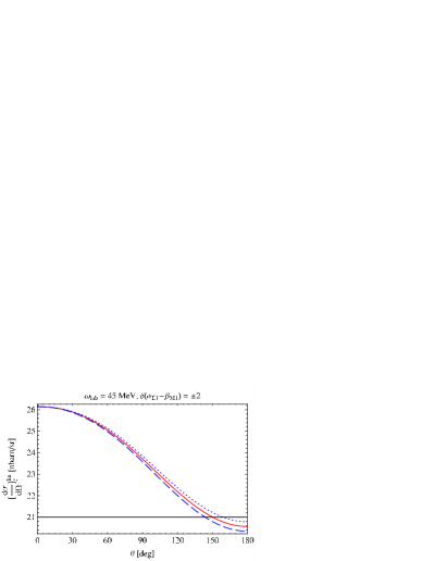
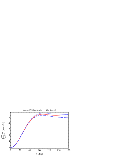
Figure 14: (Colour online) Dependence of $\left[\frac{\mathrm{d}\sigma}{\mathrm{d}\Omega}\right]^{\text{lin}}_{x}$ (left) and $\left[\frac{\mathrm{d}\sigma}{\mathrm{d}\Omega}\right]^{\text{lin}}_{y}$ (right) at $\omega_{\text{lab}}=45$ MeV (top) and $125$ MeV (bottom) on $\delta(\alpha_{E1}-\beta_{M1})=\pm 2$, with their sum constrained by the Baldin sum-rule. Notation as in Fig. 10. Notice the scale offset.

In summary, $\left[\frac{\mathrm{d}\sigma}{\mathrm{d}\Omega}\right]_{x}^{\text{lin}}$ does not appear to be a good observable to extract even the largest of the polarisabilities, while $\left[\frac{\mathrm{d}\sigma}{\mathrm{d}\Omega}\right]_{y}^{\text{lin}}$ proves to be an effective observable to extract both $\alpha_{E1}$ and $\beta_{M1}$, or the combination $\alpha_{E1}-\beta_{M1}$. It also shows sensitivity to mostly $\gamma_{M1M1}$ at higher energies. With the increased flux at HI$\gamma$S, such effects should be measurable.

V Double-polarisation Observables

New experimental techniques make it feasible to measure observables involving linearly or circularly polarised photons and a deuteron target that can be vector-polarised either along the beam axis or perpendicular to it, see eqs. (13) to (16). A first qualitative study of some effects was given in “pion-less” EFT in Ref. Chen:2004wwa . We extend the analysis of polarisation observables for circularly polarised photons by $\chi$EFT in Ch05 ; mythesis to include the sizable contributions from $NN$-rescattering and dynamical $\Delta$ effects. In addition, we demonstrate, to our knowledge for the first time, that linearly polarised beams provide an avenue to extract polarisabilities in deuteron Compton scattering.

Consider first again the effective Lagrangean (1) with a configuration in which the target is polarised parallel to the linear polarisation of the beam, cf. Fig. 9. Now, $\gamma_{E1E1}$ does not contribute to scattering under any scattering angle. Similarly, scattering off a target polarised perpendicular to a linearly polarised beam is under any angle insensitive to $\gamma_{M1M1}$. No such relations are found for circularly polarised photons on vector polarised targets. Double polarisation observables are however formulated using differences of cross-sections with different polarisations, and no straight-forward argument exists that one or more of the dipole polarisabilities as insensitive to $\Delta^{\text{lin/circ}}_{x/z}$ or $\Sigma^{\text{lin/circ}}_{x/z}$. Recall that differences and asymmetries are favoured in small count-rates since some systematic effects cancel.

As done for single-polarisation observables, we consider first sensitivity of each observable to the spin-independent polarisabilities at $\omega_{\text{lab}}=45$ and $125$ MeV, followed by sensitivity to the spin-polarisabilities at $125$ MeV. We also re-iterate that while only cross-section differences $\Delta^{\text{circ/lin}}_{x/z}$ are presented in the following, we also investigated asymmetries $\Sigma^{\text{circ/lin}}_{x/z}$, with results available in a Mathematica notebook. In general, sensitivity to polarisabilities are decreased in asymmetries, relative to signals in differences.

V.1 Polarised Target and Linearly-polarised Photons

The observable $\Delta^{\text{lin}}_{z}$, (14), describes scattering linearly polarised photons off a target polarised parallel to the beam. The best signal is obtained when the beam polarisation lies in the scattering plane.

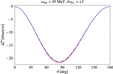
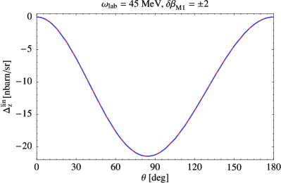
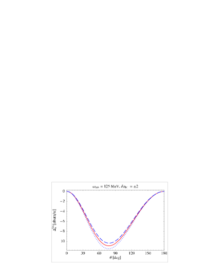
Figure 15: (Colour online) Dependence of $\Delta^{\text{lin}}_{z}$ on the spin-independent dipole polarisabilities at $\omega_{\text{lab}}=45$ MeV (top) and $\omega_{\text{lab}}=125$ MeV (bottom). Notation as in Fig. 10.

At 45 MeV, varying $\delta\alpha_{E1}=\pm 2$ causes an effect of $\lesssim\pm 0.25$ nbarn/sr at $\theta_{\text{lab}}\approx 90^{\circ}$, while this doubles at 125 MeV to a maximum of $\pm 0.5$ nbarn/sr, see Fig. 15. The effect of $\beta_{M1}$ is insignificant at 45 MeV and $\lesssim\pm 0.25$ nbarn/sr at 125 MeV, anti-correlated to that of $\alpha_{E1}$.

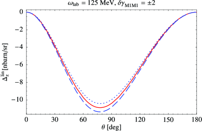
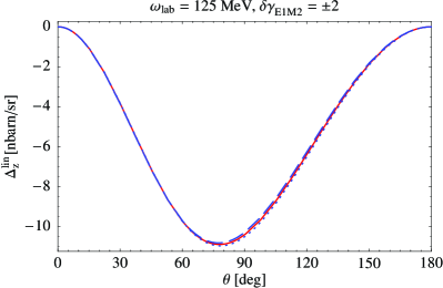
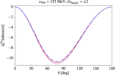
Figure 16: (Colour online) Dependence of $\Delta^{\text{lin}}_{z}$ at $\omega_{\text{lab}}=125$ MeV on the dipole spin-polarisabilities. Notation as in Figs. 10 and 11.

When the spin-polarisabilities are varied one by one by $\pm 2$ units around their central values at $\omega_{\text{lab}}=125$ MeV in Fig. 16, sensitivity to $\gamma_{M1M1}$ around $\theta_{\text{lab}}\approx 75^{\circ}$ provides with $\pm$0.5 nbarn/sr a measurably large effect, comparable but anti-correlated to that of $\alpha_{E1}$. However, a weak dependence on $\gamma_{M1E2}$ ($\pm$0.2 nbarn/sr) cannot be discounted. Since sensitivity on the other spin-polarisabilities is negligible, one can extract a linear combination of the anti-correlated polarisabilities $\gamma_{M1M1}$ and $\gamma_{M1E2}$, with the former dominating. These polarisabilities are expected to be dominated by the strongly para-magnetic $\gamma\Delta N$ coupling.

A complementary picture emerges in Figs. 17 and 18 for $\Delta^{\text{lin}}_{x}$, in which the target spin is perpendicular to the beam direction, (13).

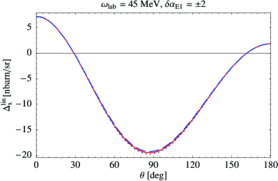
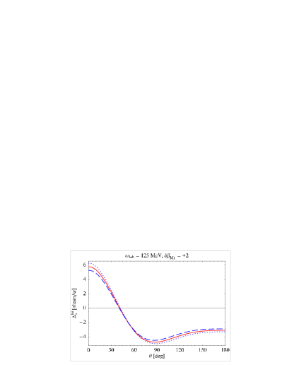
Figure 17: (Colour online) Dependence of $\Delta^{\text{lin}}_{x}$ on the spin-independent dipole polarisabilities at $\omega_{\text{lab}}=45$ MeV (top) and $\omega_{\text{lab}}=125$ MeV (bottom). Notation as in Fig. 10.

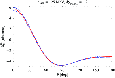
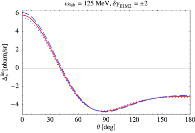
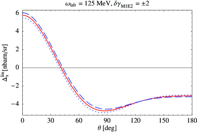
Figure 18: (Colour online) Dependence of $\Delta^{\text{lin}}_{x}$ at $\omega_{\text{lab}}=125$ MeV on the dipole spin-polarisabilities. Notation as in Figs. 10 and 11.

At 45 MeV, varying $\alpha_{E1}$ leads to an effect of $\lesssim\pm 0.2$ nbarn/sr, whereas the effect due to $\delta\beta_{M1}$ is indiscernible. At 125 MeV the maximum sensitivity to $\alpha_{E1}$ increases to $\approx\pm 0.5$ nbarn/sr, twice of the dependence on $\beta_{M1}$. At forward angles, $\Delta^{\text{lin}}_{x}$ at $\omega_{\text{lab}}=125$ MeV is equally sensitive to all spin-polarisabilities. For $\theta_{\text{lab}}\in[90^{\circ};120^{\circ}]$, contributions from $\gamma_{E1E1}$ dominate (sensitivity $\lesssim\pm 0.25$ nbarn/sr), with a modest admixture of $\gamma_{M1E2}$ which decreases to zero around $120^{\circ}$. One may thus extract a linear combination of only two spin-polarisabilities, complementary to that from $\Delta^{\text{lin}}_{z}$.

To summarise, $\alpha_{E1}$ has a sizable effect on both $\Delta^{\text{lin}}_{z}$ and $\Delta^{\text{lin}}_{x}$, bigger than the effect of $\beta_{M1}$ or any of the spin-polarisabilities. $\Delta^{\text{lin}}_{z}$ is sensitive to a combination of $\gamma_{M1M1}$ and $\gamma_{M1E2}$, while $\Delta^{\text{lin}}_{x}$ can be used to extract a combination of $\gamma_{E1E1}$ and $\gamma_{M1E2}$. Both observables are virtually in-sensitive to $\gamma_{E1M2}$.

V.2 Polarised Target and Circularly-polarised Photons

Calculations for the circularly-polarised photon observables $\Delta_{z}^{\text{circ}}$ and $\Delta_{x}^{\text{circ}}$ at $\mathcal{O}(Q^{3})$ for $\omega\sim m_{\pi}$ and without dynamical $\Delta$ were first reported in Refs. Ch05 ; mythesis . The spin-polarisabilities were given not in the basis of photon multipolarities used here but by $\gamma_{1,2,3,4}$ of the Ragusa basis Ragusa:1993rm ; see e.g. Ref. (Babusci:1998ww, , App. A) for a translation between the two. It was shown that $\Delta_{x}^{\text{circ}}$ had considerable sensitivity to some spin-polarisabilities. As discussed in Sec. III, Figs. 7 and 8, the dynamical $\Delta$ increases these effects.

Figures 19 and 20 show the dependence of the parallel polarisation asymmetry $\Delta_{z}^{\text{circ}}$ on the spin-independent and spin-polarisabilities in SSE $\chi$EFT.

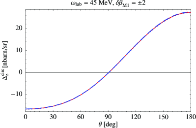
Figure 19: Colour online) Dependence of $\Delta^{\text{circ}}_{z}$ on the spin-independent dipole polarisabilities at $\omega_{\text{lab}}=45$ MeV (top) and $\omega_{\text{lab}}=125$ MeV (bottom). Notation as in Fig. 10.

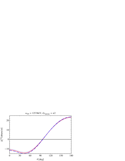
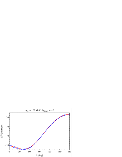
Figure 20: (Colour online) Dependence of $\Delta^{\text{circ}}_{z}$ at $\omega_{\text{lab}}=125$ MeV on the dipole spin-polarisabilities. Notation as in Figs. 10 and 11.

At 45 MeV, the sensitivity to any polarisability is less than the line thickness. At 125 MeV, sensitivity to both $\alpha_{E1}$ and $\beta_{M1}$ grows to $\pm 2.5$ nbarn/sr, with different angular dependence.

Looking back at the contribution of $\approx 7$ nbarn/sr which a dynamical $\Delta$ provides overall according to Fig. 8, it seems surprising that the sensitivity on varying $\delta\beta_{M1}=\pm 2$ in Fig. 10 is only $\pm 2.5$ nbarn/sr. This serves however to illustrate an important point on the energy-dependence of the polarisabilities and the interpretation of the variation parameters $\delta(\alpha_{E1},\beta_{M1},\gamma_{i})$. Bear in mind that the value of the dynamical polarisability is at this energy $\beta_{M1}(\omega=120\;\mathrm{MeV})\approx 7$ as seen in Ref. (Hi04, , Fig. 8). This is about $3$ to $4$ times the static value $\beta_{M1}\approx[2\dots 3]$ or its near-identical dynamical value at that energy in the version without explicit $\Delta$. Recall that $\beta_{M1}(\omega)$ is only very weakly $\omega$-dependent without $\Delta$s. Switching off effects from the magnetic polarisability completely does therefore at this energy not correspond to choosing $\delta\beta_{M1}=-2$ or $-3$, but to $\delta\beta_{M1}=-7$. Switching off the $\Delta$-effects corresponds to $\delta\beta_{M1}=-5$. Re-scaling the variation in Fig. 19 accordingly and keeping in mind that the amplitudes are to a good approximation linear in the polarisabilities, one indeed recovers the result of Fig. 8. We therefore re-iterate what we already noted in Sec. II.3: Varying the polarisabilities by values $\delta(\alpha_{E1},\beta_{M1},\gamma_{i})$ is equivalent to varying the static polarisabilities by the same amount only if the energy-dependence of the polarisabilities follows the $\chi$EFT prediction. If not, the variations test deviations to experiments at fixed energy.

Sensitivity of $\Delta_{z}^{\text{circ}}$ to the spin-polarisabilities is $\lesssim\pm 0.7$ nbarn/sr at 125 MeV, most notably at forward and backward angles. Angular dependence does not provide a clean tool to dis-entangle different spin-polarisabilities. Sensitivity to $\gamma_{E1E1}$ and $\gamma_{E1M2}$ is again equal but opposite, while that to $\gamma_{M1M1}$, $\gamma_{E1M2}$ and $\gamma_{M1E2}$ is largely additive.

The dependence of $\Delta_{z}^{\text{circ}}$ was also studied in “pion-less” EFT Chen:2004wwa by comparing to the case when the spin-polarisabilities are absent. The range of applicability of this theory in which the pion is integrated out as heavy is however limited to typical momenta well below the pion mass and thus to typical photon energies $\omega\lesssim m_{\pi}^{2}/M\approx 20\;\mathrm{MeV}$. As noted by the authors, their predictions at cm energies of $70$ and $90$ MeV are therefore only of qualitative interest. At $70$ MeV, the discrepancy to the results presented here rises to $\gtrsim 20\%$ and is most pronounced at back-angles. This may be attributed to the fact that the dynamical $\Delta$ increases $\Delta_{z}^{\text{circ}}$, see Fig. 8. It is interesting that their results at $30$ and $50$ MeV are still very similar to those with dynamical pions and $\Delta$s, even thought these energies are strictly speaking beyond the breakdown scale of the EFT without pions. This holds also for their results on $\Sigma_{z}^{\text{circ}}$. Their $\Sigma_{x}^{\text{circ}}$ is however larger by about $20$% in the peak and has a less pronounced concave flank at forward angles, cf. Fig. 7.

The parallel polarisation asymmetry $\Delta_{x}^{\text{circ}}$ is only minimally sensitive to polarisabilities at $45$ MeV, see Figs. 21 and 22.

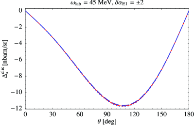
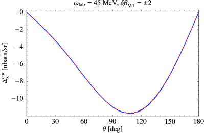
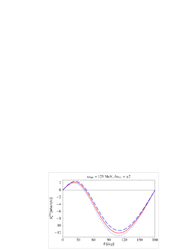
Figure 21: (Colour online) Dependence of $\Delta^{\text{circ}}_{x}$ on the spin-independent dipole polarisabilities at $\omega_{\text{lab}}=45$ MeV (top) and $\omega_{\text{lab}}=125$ MeV (bottom). Notation as in Fig. 10.

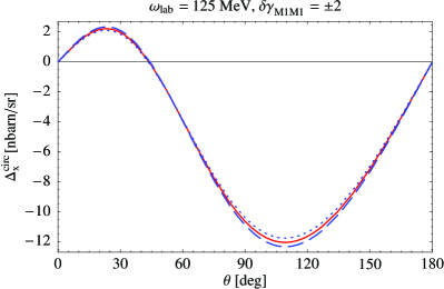
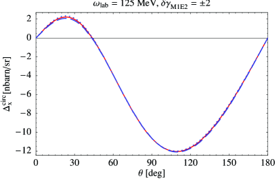
Figure 22: (Colour online) Dependence of $\Delta^{\text{circ}}_{x}$ at $\omega_{\text{lab}}=125$ MeV on the dipole spin-polarisabilities. Notation as in Figs. 10 and 11.

At 125 MeV, dependence on $\alpha_{E1}$ is $\lesssim\pm 0.8$ nbarn/sr, and on $\beta_{M1}$ $\lesssim\pm 0.6$ nbarn/sr. The two can be dis-entangled, as contributions from $\beta_{M1}$ are zero at $\theta_{\text{lab}}\approx 60^{\circ}$. Of the spin-polarisabilities, $\delta\gamma_{E1E1}$ causes a maximum change of $\lesssim\pm 0.6$ nbarn/sr, i.e. about $\frac{3}{4}$ of changing $\alpha_{E1}$, but with opposite sign. Varying $\gamma_{M1M1}$ induces a $\lesssim\pm 0.3$ nbarn/sr effect, equal in magnitude and sign to that of $\beta_{M1}$. A weak but noticeable angular dependence may allow dis-entangling $\gamma_{M1E2}$ at forward angles.

Asymmetries with circularly polarised beams offer thus a sensitivity to the spin-polarisabilities which is weaker or at most comparable to those of linearly polarised ones. There is no realistic opportunity to measure an observable which is sensitive to the linear combination of less than three spin-polarisabilities. In contradistinction, linear beam polarisation offers the chance to measure linear combinations of only two spin-polarisabilities, with the others being practically absent. For all double-polarisation observables, the spin-independent dipole polarisabilities $\alpha_{E1}$ and $\beta_{M1}$ must be known reliably, as their effects over-shadow those of the spin-polarisabilities at all energies.

VI Summary and Outlook

We investigated elastic deuteron Compton scattering with a polarised beam and/or target at next-to-leading order, $\mathcal{O}(\epsilon^{3})$ within Chiral Effective Field Theory in the photon energy range between zero and $125$ MeV (lab), using the power-counting scheme of Hildebrandt et al. Hi05 ; Hi05b . This systematic, model-independent approach contains dynamical $\Delta(1232)$ degrees of freedom in the Small Scale Expansion and contributions from intermediate-state $NN$-rescattering, leading to strong para-magnetic effects and the correct Thomson limit, respectively. Both have sizeable effects on polarisation observables: The $\Delta$-isobar is significant at higher energies, while the intermediate $NN$-rescattering states are significant throughout the energy range. These are thus important ingredients of any theoretical description of deuteron Compton scattering at these energies. They are needed both for consistency of the theory and for matching to well-established data.

Single and double polarisation observables are quite sensitive to the electric and magnetic polarisabilities, as shown in Sec. V. Since these can also be directly extracted from unpolarised scattering, as shown e.g. in Refs. Be02 ; Be04 ; Hi05 ; Hi05b , it is imperative that they be determined to better accuracy so as not to taint an extraction of the so-far experimentally nearly un-determined spin-polarisabilities from polarised experiments. Our results also show that some of the double-polarisation observables are sensitive to different linear combinations of the spin-polarisabilities at energies $\gtrsim 80$ MeV. The linear-beam polarisation observables $\Delta^{\text{lin}}_{x,z}$ with target polarisations parallel or perpendicular to the beam proved most promising from the theorist’s point of view, since they are each at high energies and for certain, experimentally feasible angles dominated by linear combinations of only two spin-polarisabilities.

The cross-section of a linearly polarised photon on an un-polarised target can be used to “switch off” or maximise dependence on one of the spin-independent polarisabilities, as demonstrated in Sec. IV. When the beam polarisation is perpendicular to the scattering plane, the signal of a combination of spin-polarisabilities is particularly strong. Even then, the spin-independent polarisabilities must be known with sufficient accuracy.

In view of these findings, we advocate the following strategy:

1. Since an accurate extraction of the electric and magnetic polarisabilities is central to extracting the spin-polarisabilities, it is crucial to perform a number of relatively low-energy experiments ($\lesssim 70$ MeV). In these, spin-polarisabilities are negligible but spin-independent polarisabilities can be determined to high accuracy. Besides an unpolarised deuteron Compton scattering experiment at MAXlab whose analysis is in progress Feldman:2008zz ; Feldman2 , experiments at HI$\gamma$S have been approved Weller ; Weller:2009zza using a polarised beam. Some of the single and double-polarisation observables can also be used to that purpose. Such data will not only serve as stepping-stone for determinations of spin-polarisabilities; comparing the iso-scalar spin-independent polarisabilities thus extracted with the spin-independent polarisabilities of the proton will also reveal differences between the proton and neutron response to external electro-magnetic fields.

2. With $\alpha_{E1}$ and $\beta_{M1}$ better known, a series of concurrent polarised and unpolarised measurements at higher energies will allow the extraction of the spin-polarisabilities. The best chances are presumably offered by double-polarisation observables at $\gtrsim$ 100 MeV but below the pion-production threshold. For example, $\Delta_{x}^{\text{lin}}$ and $\Delta_{x}^{\text{circ}}$ are sensitive to different linear combinations of the four spin-polarisabilities; and at some angles, $\Delta_{x}^{\text{lin}}$ and $\Delta_{z}^{\text{lin}}$ can be used to determine linear combinations of only two spin-polarisabilities. Measuring several linear combinations makes it possible to disentangle the four independent spin-polarisabilities.

Ideally, a multipole-analysis of $4+1$ experiments at different angles suffices to over-determine the $4$ spin-polarisabilities – if the data are of an unprecedented high accuracy which is presumably not feasible today. $\gamma_{E1E1}$ and $\gamma_{M1M1}$ can to a good approximation be extracted uniquely from $\Delta_{x}^{circ}$ and $\Delta_{z}^{lin}$, respectively. However, a larger number of independent data will be necessary to account for the high complexity of these experiments and for the fact that no clear-cut observables exist for the “mixed” spin-polarisabilities $\gamma_{E1M2}$ and $\gamma_{M1E2}$. In each experiment, the accuracy achievable and the observables and kinematics most suited strongly depend on geometry and acceptance of the setup.

A concerted effort of planned and approved experiments at $\omega_{\text{lab}}\lesssim 200\;\mathrm{MeV}$ is indeed under way, e.g. polarised photons on polarised protons, deuterons and ³He at TUNL/HI$\gamma$S Weller:2009zza ; Weller ; Miskimen ; Miskimentalk ; Gao ; Ahmed ; polarised photons on polarised protons at MAMI AhrensBeckINT08 . The unpolarised experiment on the deuteron at MAXlab over a wide range of energies and angles is being analysed Feldman:2008zz ; Feldman2 . At present, only 28 (un-polarised) data exist for the deuteron in an energy range $\omega_{\text{lab}}\in[49;94]$ MeV and with error-bars on the order of $15\%$. It was shown in Refs. mythesis ; Ch07 ; Sh08 that one can in addition extract a subset of the neutron polarisabilities from elastic Compton scattering off ³He, with an experiment at HI$\gamma$S approved Gao . Since the total charge is doubled in this target, sensitivity to polarisabilities is increased by larger interference of non-structure and polarisability amplitudes. On the other hand, restoration of the Thomson limit needs to be addressed for ³He. Other avenues may include quasi-free measurements on light nuclei.

To facilitate planning and analysis of such experiments, we have made our detailed results for unpolarised and polarised observables in deuteron Compton scattering available as interactive Mathematica 7.0 notebook (email to hgrie@gwu.edu). It lists and plots both energy- and angle-dependences of cross-sections and all the asymmetries as well as cross-section differences from $10$ to $\approx 120$ MeV in both the cm and lab systems, including the sensitivities to varying the spin-independent and spin-dependent dipole polarisabilities independently and with the Baldin sum rule constraint. It thus provides a more thorough and efficient tool to investigate sensitivities and impacts both of experimental constraints and of theoretical information like the Baldin sum rule (6).

In the long run, a global multipole-analysis at fixed energies of a database that includes both polarised and un-polarised elastic Compton scattering high-accuracy measurements on the proton, deuteron and ³He, from low to high energies at various angles, gives an unambiguous extraction of the two spin-independent and four spin-dependent polarisabilities, for both the proton and neutron. That such a multipole-analysis is feasible has been advocated in hgrieproc ; Miskimentalk . First results were reported based on the wealth of unpolarised proton data hgrieproc . High-quality data will allow one to zoom in on the proton-neutron differences, which according to $\chi$EFT stem from chiral-symmetry breaking pion-nucleon interactions; and provide information on the spin-polarisabilities which parameterise the detailed response of the nucleon spin degrees of freedom in external electro-magnetic fields.

Future improvement in our deuteron Compton scattering calculations include: transition to a chirally fully consistent deuteron wave-function and $NN$-potential; implementing the kinematically correct pion-production threshold to extend our reach into the $\Delta$-resonance region; and a detailed assessment of residual theoretical uncertainties. The work presented here is part of a wider effort to describe elastic Compton scattering on the proton, deuteron and ³He from the Thomson limit to well into the $\Delta$-resonance region in one model-independent, unified framework. We focus at present on improving the accuracy of current calculations by a full next-to-next-to-leading order calculation with nucleons, pions and the $\Delta(1232)$ as dynamical, effective degrees of freedom Griesshammer:2009pq ; McGovern:2009sw ; allofus .

References

- (1) H. W. Grießhammer, Prog. Part. Nucl. Phys. 55, 215 (2005) [arXiv:nucl-th/0411080].
- (2) B. R. Holstein, D. Drechsel, B. Pasquini and M. Vanderhaeghen, Phys. Rev. C 61, 034316 (2000) [arXiv:hep-ph/9910427].
- (3) D. Drechsel, B. Pasquini and M. Vanderhaeghen, Phys. Rept. 378, 99 (2003) [arXiv:hep-ph/0212124].
- (4) M. Schumacher, Prog. Part. Nucl. Phys. 55, 567 (2005) [arXiv:hep-ph/0501167].
- (5) D. R. Phillips, J. Phys. G 36, 104004 (2009) [arXiv:0903.4439 [nucl-th]].
- (6) H. R. Weller, M. W. Ahmed, H. Gao, W. Tornow, Y. K. Wu, M. Gai and R. Miskimen, Prog. Part. Nucl. Phys. 62 (2009) 257.
- (7) H. Weller et al., HIGS-E-18-09; H. Weller, private communication.
- (8) R. Miskimen et al., HIGS-E-06-09; R. Miskimen, private communication.
- (9) R. Miskimen, Measuring the Spin-Polarizabilities of the Proton at HIS, presentation at the INT workshop on Soft Photons and Light Nuclei, 17 June 2008, and private communication.
- (10) H. Gao et al., HIGS-E-07-10; H. Gao, private communication.
- (11) M. Ahmed et al., HIGS-E-06-10; M. Ahmed, private communication.
- (12) R. Beck, Nucleon Compton Scattering at MAMI, talk at the INT workshop on Soft Photons and Light Nuclei, 17 June 2008; V. Ahrens and. R. M. Annand, private communication.
- (13) G. Feldman et al., Few Body Syst. 44, 325 (2008).
- (14) MAXlab experiment NP-006 (http://www.maxlab.lu.se/kfoto/ExperimentalProgram/PAC_info.html); G. Feldman, K. Fissum and L. Myers, private communication.
- (15) R. P. Hildebrandt, Ph. D. Thesis, [arXiv:nucl-th/0512064].
- (16) R. P. Hildebrandt, H. W. Grießhammer, and T. R. Hemmert, Eur. Phys. J. A in press [arXiv:nucl-th/0512063].
- (17) R. P. Hildebrandt, H. W. Grießhammer, T. R. Hemmert, and D. R. Phillips, Nucl. Phys. A 748, 573 (2005) [arXiv:nucl-th/0405077].
- (18) K. Kossert et al., Eur. Phys. J. A 16, 259 (2003) [arXiv:nucl-ex/0210020].
- (19) M. Lundin et al., Phys. Rev. Lett. 90, 192501 (2003) [arXiv:nucl-ex/0204014].
- (20) S. R. Beane, M. Malheiro, D. R. Phillips and U. van Kolck, Nucl. Phys. A 656, 367 (1999) [arXiv:nucl-th/9905023].
- (21) S. R. Beane, M. Malheiro, J. A. McGovern, D. R. Phillips and U. van Kolck, Phys. Lett. B 567, 200 (2003) [Erratum-ibid. B 607, 320 (2005)] [arXiv:nucl-th/0209002].
- (22) S. R. Beane, M. Malheiro, J. A. McGovern, D. R. Phillips and U. van Kolck, Nucl. Phys. A 747, 311 (2005) [arXiv:nucl-th/0403088]. ).
- (23) A. Alexandru and F. X. Lee, [arXiv:0911.2520 [hep-lat]].
- (24) M. Engelhardt, PoS LAT2009, 128 (2009) [arXiv:1001.5044 [hep-lat]].
- (25) W. Detmold, B. C. Tiburzi and A. Walker-Loud, Phys. Rev. D 81, 054502 (2010) [arXiv:1001.1131 [hep-lat]].
- (26) H. W. Grießhammer and T. R. Hemmert, Phys. Rev. C 65, 045207 (2002) [arXiv:nucl-th/0110006].
- (27) R. P. Hildebrandt, H. W. Grießhammer, T. R. Hemmert, and B. Pasquini, Eur. Phys. J. A 20, 293 (2004) [arXiv:nucl-th/0307070].
- (28) R. P. Hildebrandt, H. W. Grießhammer and T. R. Hemmert, Eur. Phys. J. A 20 (2004) 329 [arXiv:nucl-th/0308054].
- (29) V. Pascalutsa and D. R. Phillips, Phys. Rev. C 67, 055202 (2003) [arXiv:nucl-th/0212024].
- (30) V. Lensky and V. Pascalutsa, Eur. Phys. J. C 65, 195 (2010) [arXiv:0907.0451 [hep-ph]].
- (31) V. Pascalutsa and D. R. Phillips, Phys. Rev. C 68, 055205 (2003) [arXiv:nucl-th/0305043].
- (32) A. M. Sandorfi, M. Khandaker and C. S. Whisnant, Phys. Rev. D 50, 6681 (1994).
- (33) M. Gell-Mann, M. L. Goldberger and W. E. Thirring, Phys. Rev. 95, 1612 (1954).
- (34) K. B. Vijaya Kumar, J. A. McGovern and M. C. Birse, [arXiv:hep-ph/9909442].
- (35) T. R. Hemmert, [arXiv:nucl-th/0101054].
- (36) H. Arenhövel, Z. Phys. A 297, 129 (1980).
- (37) M. Weyrauch and H. Arenhövel, Nucl. Phys. A 408, 425 (1983).
- (38) T. Wilbois, P. Wilhelm, and H. Arenhövel, Few Body Sys. Suppl. 9, 263 (1995).
- (39) M. I. Levchuk, and A. I. L’vov, Few Body Sys. Suppl. 9, 239 (1995).
- (40) M. I. Levchuk and A. I. L’vov, Nucl. Phys. A 674, 449 (2000).
- (41) M. I. Levchuk and A. I. L’vov, Nucl. Phys. A 684, 490 (2001) [arXiv:nucl-th/0010059].
- (42) J. J. Karakowski, and G. A. Miller, Phys. Rev. C60, 014001 (1999).
- (43) D. Choudhury, A. Nogga and D. R. Phillips, Phys. Rev. Lett. 98, 232303 (2007) [arXiv:nucl-th/0701078].
- (44) D. Shukla, A. Nogga and D. R. Phillips, Nucl. Phys. A 819, 98 (2009) [arXiv:0812.0138 [nucl-th]].
- (45) D. Choudhury, Ph.D. Thesis Ohio University (2006).
- (46) J. W. Chen, X. d. Ji and Y. c. Li, Phys. Rev. C 71, 044321 (2005) [arXiv:nucl-th/0408004].
- (47) D. Choudhury and D. R. Phillips, Phys. Rev., C 71, 044002 (2005).
- (48) T. R. Hemmert, B. R. Holstein and J. Kambor, Phys. Rev. D 55, 5598 (1997).
- (49) T. R. Hemmert, B. R. Holstein, J. Kambor and G. Knöchlein, Phys. Rev. D 57, 5746 (1998).
- (50) H. W. Grießhammer and D. Shukla, [arXiv:0910.0053 [nucl-th]].
- (51) V. Olmos de Leon et al., Eur. Phys. J. A 10, 207 (2001).
- (52) R. A. Arndt, W. J. Briscoe, I. I. Strakovsky and R. L. Workman, Phys. Rev. C66, 055213 (2002).
- (53) H. W. Grießhammer, In the Proceedings of 11th International Conference on Meson-Nucleon Physics and the Structure of the Nucleon (MENU 2007), Julich, Germany, 10-14 Sep 2007, p. 141 [arXiv:0710.2924 [nucl-th]].
- (54) H. W. Grießhammer, forthcoming.
- (55) J.L. Friar, Ann. of Phys. 95, 170 (1975).
- (56) S. Weinberg, Phys. Lett. B 251, 288 (1990).
- (57) S. Weinberg, Nucl. Phys. B 363, 3 (1991).
- (58) R.B. Wiringa, V.G. Stoks and R. Schiavilla, Phys. Rev. C 51, 38 (1995).
- (59) E. Epelbaum, W. Glöckle and U.-G. Meißner, Eur. Phys. J. A 19, 125 (2004).
- (60) E. Epelbaum, W. Glöckle and U.-G. Meißner, Eur. Phys. J. A 19, 401 (2004).
- (61) V.G. Stoks, R.A. Klomp, C.P. Terheggen and J.J. de Swart, Phys. Rev. C 49, 2950 (1994).
- (62) S. Pastore, L. Girlanda, R. Schiavilla, M. Viviani and R. B. Wiringa, Phys. Rev. C 80, 034004 (2009) [arXiv:0906.1800 [nucl-th]].
- (63) S. Kolling, E. Epelbaum, H. Krebs and U. G. Meißner, Phys. Rev. C 80, 045502 (2009) [arXiv:0907.3437 [nucl-th]].
- (64) H. Grießhammer, J. McGovern, D. R. Phillips, D. Shukla, work in progress.
- (65) D.L. Hornidge et al., Phys. Rev. Lett. 84, 2334 (2000).
- (66) L. C. Maximon, Phys. Rev. C 39 (1989) 347.
- (67) S. Ragusa, Phys. Rev. D 47, 3757 (1993).
- (68) D. Babusci, G. Giordano, A. I. L’vov, G. Matone and A. M. Nathan, Phys. Rev. C 58 (1998) 1013 [arXiv:hep-ph/9803347].
- (69) J. A. McGovern, H. W. Grießhammer, D. R. Phillips and D. Shukla, [arXiv:0910.1184 [nucl-th]].