Field-induced decay dynamics in square-lattice antiferromagnet

Abstract

Dynamical properties of the square-lattice Heisenberg antiferromagnet in applied magnetic field are studied for arbitrary value $S$ of the spin. Above the threshold field for two-particle decays, the standard spin-wave theory yields singular corrections to the excitation spectrum with logarithmic divergences for certain momenta. We develop a self-consistent approximation applicable for $S\geq 1$, which avoids such singularities and provides regularized magnon decay rates. Results for the dynamical structure factor obtained in this approach are presented for $S=1$ and $S=5/2$.

I Introduction

The square-lattice Heisenberg antiferromagnet is an important model system in quantum magnetism. Manousakis91 Theoretical studies of this model have provided deep insights into the role of low-dimensionality in the static and dynamical properties of the many-body spin systems. Recently, there has been a growing interest in the effect of magnetic field in the dynamics of quantum antiferromagnets. The strong-field regime is now reachable for a number of layered square-lattice materials with moderate strength of exchange coupling between spins. Woodward02 ; Lancaster07 ; Coomer07 ; Tsyrulin09 In addition, new field-induced dynamical effects can be present in the antiferromagnets with other lattice geometries Coldea02 ; Nakatsuji05 as well as in the gapped quantum spin systems near the condensation field for triplet excitations. Affleck91 ; Affleck92 ; Mila98 ; Giamarchi99 ; Nikuni00 ; Jaime04 ; Regnault06

The ground-state properties of the square-lattice antiferromagnet in a finite field conform with the semiclassical picture of spins gradually tilted towards the field direction, Zhitomirsky98 see Fig. 1. On the other hand, excitation spectrum and dynamical properties are expected to undergo rather dramatic transformation. Zhitomirsky99 ; Olav08 ; Luscher09 Following the prediction of the field-induced spontaneous magnon decays in Ref. Zhitomirsky99, , there is an ongoing search for suitable spin-1/2 square-lattice materials Woodward02 ; Lancaster07 ; Coomer07 ; Tsyrulin09 to investigate such an effect. The existence of substantial damping in the magnon spectrum of the square-lattice Heisenberg model in a field has been recently verified by the Quantum Monte Carlo Olav08 (QMC) and the Exact Diagonalization Luscher09 numerical study. Other theoretical aspects of the behavior of the quantum square-lattice antiferromagnet (SAFM) in applied field have also been addressed. Kreisel08 ; Syromyat09 ; Chernyshev09b

In this paper, we extend previous work of two of us Zhitomirsky99 and provide a comprehensive theoretical investigation of the dynamics of the nearest-neighbor Heisenberg SAFM including detailed calculation of the $1/S$ correction to the energy spectrum in external field, kinematic analysis of the field-induced two-magnon decays, and self-consistent treatment of magnon decay rates for systems with $S\geq 1$.

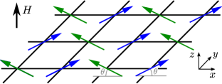
Figure 1: (Color online) Canted spin structure of the square-lattice Heisenberg antiferromagnet in external magnetic field.

The model spin Hamiltonian is

$$\hat{\cal H}=J\sum_{\langle ij\rangle}\mathbf{S}_{i}\cdot\mathbf{S}_{j}-H\sum_{i}S_{i}^{z}\ ,$$ (1)

where $J$ stands for the nearest-neighbor exchange coupling constant and $H$ is the external magnetic field in units of $g\mu_{B}$.

The standard spin-wave theory works quite well for the SAFM in zero field. Manousakis91 ; Hamer92 ; Igarashi92 ; Canali93 ; Igarashi05 Surprisingly enough, in high magnetic fields one encounters strong singularities in the spin-wave corrections to the dynamical properties of the SAFM, which arise due to spontaneous magnon decays above the threshold field $H^{*}\approx 0.75H_{s}$. Zhitomirsky99 Singular behavior of the spectrum signifies a breakdown of the perturbative $1/S$ expansion and requires a regularization. The aim of this work is to develop a self-consistent approximation which yields the spectrum that is free from the essential singularities.

Within the conventional spin-wave approach, the gapless Goldstone branch is preserved only if all quantum corrections to the spectrum of the same order in $1/S$ are taken into account. This represents an obvious difficulty for any self-consistent calculation, which typically involves summation of a certain infinite subset of perturbation series. The basic idea of the present work is to neglect the real part of the spectrum corrections completely and to perform the self-consistent calculation only in the imaginary part of the magnon self-energy. Such an approach is justified if the real part of corrections is small, which is the case for $S\geq 1$ for the model (1). Utilizing this self-consistent scheme we obtain explicit results for the magnon decay rates and the dynamical structure factor of SAFMs with $S=1$ and $S=5/2$.

The paper is organized as follows. Technical details of the spin-wave theory in magnetic field are provided in Sec. II together with explicit calculation of the quantum correction for the spin-1/2 SAFM. The kinematic analysis of the field-induced magnon decays and associated singularities is presented in Sec. III. The self-consistent theory is described in Sec. IV, where the results for the dynamical structure factor are also included. Sec. V contains our conclusions. The asymptotic form for the decay rate of low-energy magnons is derived in Appendix A and an extension of the kinematic analysis to anisotropic antiferromagnets is given in Appendix B.

II Spin-Wave Expansion

In this section we provide necessary details of the standard spin-wave formalism as applied to two-sublattice antiferromagnets in external magnetic field at zero temperature. Zhitomirsky98 ; Zhitomirsky99 ; Chernyshev09b The first essential step is to quantize spin components in the rotating frame $(x_{i},y_{i},z_{i})$ such that the local $\hat{\bf z}_{i}$ axis points in the direction of each magnetic sublattice. In the case of the square-lattice model the ground state in zero magnetic field is the collinear Néel order characterized by the wave-vector $\mathbf{Q}=(\pi,\pi)$. In a finite magnetic field spins cant towards the field direction by an angle $\theta$, see Fig. 1. Spin components in the laboratory frame $(x_{0},y_{0},z_{0})$ are related to those in the local frame by

$$S_{i}^{x_{0}} = S_{i}^{x}\sin\theta+S_{i}^{z}e^{i{\bf Q}\cdot{\bf r}_{i}}\cos\theta\ ,\quad S_{i}^{y_{0}}=S_{i}^{y}\ ,$$

$$S_{i}^{z_{0}} = -S_{i}^{x}e^{i{\bf Q}\cdot{\bf r}_{i}}\cos\theta+S_{i}^{z}\sin\theta\ .$$ (2)

The above representation allows us to introduce only one type of bosons via the standard Holstein-Primakoff transformation. HP Substituting (2) into Eq. (1) and expanding square-roots one obtains bosonic Hamiltonian as a sum $\hat{\cal H}=\sum_{n=0}^{\infty}\hat{\cal H}_{n}$, each term being of the $n$-th order in bosonic operators and carrying an explicit factor $S^{2-n/2}$. For large spins this form provides the basis for the $1/S$ expansion.

Minimization of the classical energy $\hat{\cal H}_{0}$ determines the canting angle

$$\sin\theta=H/H_{s}\quad\textrm{with}\quad H_{s}=8JS\ .$$ (3)

The linear terms given by $\hat{\cal H}_{1}$ vanish for this choice of $\theta$ and expansion begins with the quadratic terms

$$\hat{\cal H}_{2} = H\sin\theta\sum_{i}a_{i}^{\dagger}a_{i}+JS\sum_{\langle ij\rangle}\Bigl{[}\cos 2\theta\,(a^{\dagger}_{i}a_{i}+a^{\dagger}_{j}a_{j})$$ (4)

$$+ \sin^{2}\!\theta\,(a^{\dagger}_{i}a_{j}+a^{\dagger}_{j}a_{i})-\cos^{2}\!\theta\,(a^{\dagger}_{i}a^{\dagger}_{j}+a_{j}a_{i})\Bigr{]}\,.$$

Performing successive Fourier and Bogolyubov transformations, the latter being defined as

$$a_{\bf k}=u_{\bf k}b_{\bf k}+v_{\bf k}b^{\dagger}_{-\bf k}\ ,$$

we obtain the diagonal form of $\hat{\cal H}_{2}$:

$$\hat{\cal H}_{2}=\sum_{\bf k}\epsilon_{\bf k}b_{\bf k}^{\dagger}b_{\bf k}+\frac{1}{2}\sum_{\bf k}\bigl{(}\epsilon_{\bf k}-A_{\bf k}\bigr{)}$$ (5)

with

$$\epsilon_{\bf k}=4JS\sqrt{(1+\gamma_{\bf k})(1-\cos 2\theta\gamma_{\bf k})}=4JS\omega_{\bf k}\ ,$$ (6)

$$A_{\bf k}=4JS(1+\sin^{2}\!\theta\,\gamma_{\bf k})\ ,\quad\quad u_{\bf k}^{2},v_{\bf k}^{2}=\frac{A_{\bf k}\pm\epsilon_{\bf k}}{2\epsilon_{\bf k}}\ ,$$

and $\gamma_{\bf k}=\frac{1}{2}(\cos k_{x}+\cos k_{y})$. The magnon energy in the harmonic (or linear spin-wave) approximation is given by $\epsilon_{\bf k}$. The field-induced planar anisotropy opens a gap at ${\bf k}=0$, while an acoustic branch is preserved for $\bf k\rightarrow Q$.

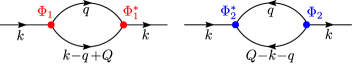
Figure 2: (Color online) The lowest-order normal self-energies generated by the decay (left) and by the source (right) vertex.

The lowest-order quantum correction to the magnon energy is determined by two types of anharmonicities, cubic and quartic. The cubic term, which originates from the coupling between transverse and longitudinal fluctuations in the canted spin structure, is given by

$$\hat{\cal H}_{3} = \sqrt{\frac{S}{2}}\Bigl{[}J\sin 2\theta\sum_{i,j}e^{i{\bf Q}{\bf r}_{i}}(a^{\dagger}_{i}+a_{i})a^{\dagger}_{j}a_{j}$$

$$+ \cos\theta\Bigl{(}2J\sin\theta-\frac{H}{4S}\Bigr{)}\sum_{i}e^{i{\bf Q}{\bf r}_{i}}\bigl{(}a^{\dagger}_{i}n_{i}+n_{i}a_{i}\bigr{)}\Bigr{]}$$

with $n_{i}=a^{\dagger}_{i}a_{i}$. The quartic term is

$$\hat{\cal H}_{4} = J\sum_{\langle ij\rangle}\Bigl{\{}\frac{1}{4}\cos^{2}\!\theta\,\bigl{[}(n_{i}+n_{j})a_{i}a_{j}+{\rm h.\,c.}\bigr{]}$$

$$- n_{i}n_{j}\cos 2\theta-\frac{1}{4}\sin^{2}\!\theta\,\bigl{[}a^{\dagger}_{i}(n_{i}+n_{j})a_{j}+{\rm h.\,c.}\bigr{]}\Bigr{\}}\ .$$

The frequency-independent $1/S$ correction to the magnon energy due to $\hat{\cal H}_{4}$ is most easily found by performing the Hartree-Fock decoupling in Eq. (II) with the following mean-field averages Oguchi60

$$n=\langle a_{i}^{\dagger}a_{i}\rangle=\sum_{\bf k}v_{\bf k}^{2}\,,\ \ m=\langle a_{i}^{\dagger}a_{j}\rangle=\sum_{\bf k}\gamma_{\bf k}v_{\bf k}^{2}\,,$$ (9)

$$\delta=\langle a_{i}^{2}\rangle=\sum_{\bf k}u_{\bf k}v_{\bf k}\,,\ \ \Delta=\langle a_{i}a_{j}\rangle=\sum_{\bf k}\gamma_{\bf k}u_{\bf k}v_{\bf k}\ .$$

The frequency-dependent corrections from quartic anharmonicities appear only in the next order in $1/S$ and are not considered here.

The role of the cubic anharmonicity is twofold. First, the Hartree-Fock decoupling in Eq. (II) yields quantum correction to the canting angle: Zhitomirsky98

$$\sin\bar{\theta}=\sin{\theta}\Bigl{[}1+\frac{1}{S}(n-m-\Delta)\Bigr{]}\ .$$ (10)

Substituting $\sin\bar{\theta}$ back into Eq. (4) one obtains another frequency-independent correction to the spectrum. The combined Hartree-Fock correction, which includes the above two contributions, reads as

$$\delta\epsilon^{(1)}_{\bf k} = \frac{4J}{\omega_{\bf k}}\Bigl{[}\Delta-n+\sin^{2}\!\theta(\Delta+m)(1-2\gamma_{\bf k}\cos^{2}\!\theta)$$

$$+ \gamma_{\bf k}^{2}\bigl{\{}n-\Delta-m+\cos 2\theta\,(\Delta\sin^{2}\!\theta+m\cos^{2}\!\theta)\bigr{\}}\Bigr{]}$$

with $\omega_{\bf k}$ being the dimensionless magnon energy, see Eq. (6).

The second contribution is due to the remaining fluctuating terms in $\hat{\cal H}_{3}$ described by three-magnon processes:

$$\hat{V}_{3}^{(1)} = \frac{1}{2!}\sum_{{\bf k},{\bf q}}\Phi_{1}({\bf k},{\bf q})\>\Bigl{[}b^{\dagger}_{\bf k-q+Q}b^{\dagger}_{\bf q}b_{\bf k}+{\rm h.\,c.}\Bigr{]},$$ (12)

$$\hat{V}_{3}^{(2)} = \frac{1}{3!}\sum_{{\bf k},{\bf q}}\Phi_{2}({\bf k},{\bf q})\>\Bigl{[}b^{\dagger}_{\bf k}b^{\dagger}_{\bf q}b^{\dagger}_{\bf Q-k-q}+{\rm h.\,c.}\Bigr{]}.$$ (13)

Decay and source vertices are given explicitly by

$$\Phi_{1,2}({\bf k},{\bf q}) = -H\cos{\theta}\;\widetilde{\Phi}_{1,2}({\bf k},{\bf q})/\sqrt{2SN}\ ,$$ (14)

$$\widetilde{\Phi}_{1}(\mathbf{k},\mathbf{q}) = \gamma_{\mathbf{k}}(u_{\mathbf{k}}+v_{\mathbf{k}})(u_{\mathbf{q}}v_{\mathbf{k-q+Q}}\!+v_{\mathbf{q}}u_{\mathbf{k-q+Q}})$$

$$+ \gamma_{\mathbf{q}}(u_{\mathbf{q}}+v_{\mathbf{q}})(u_{\mathbf{k}}u_{\mathbf{k-q+Q}}\!+v_{\mathbf{k}}v_{\mathbf{k-q+Q}})$$

$$+ \gamma_{\mathbf{k-q+Q}}(u_{\mathbf{k-q+Q}}\!+\!v_{\mathbf{k-q+Q}})(u_{\mathbf{k}}u_{\mathbf{q}}\!+\!v_{\mathbf{k}}v_{\mathbf{q}}),$$

$$\widetilde{\Phi}_{2}(\mathbf{k},\mathbf{q}) = \gamma_{\mathbf{k}}(u_{\mathbf{k}}+v_{\mathbf{k}})(u_{\mathbf{q}}v_{\mathbf{k+q-Q}}\!+v_{\mathbf{q}}u_{\mathbf{k+q-Q}})$$

$$+ \gamma_{\mathbf{q}}(u_{\mathbf{q}}+v_{\mathbf{q}})(u_{\mathbf{k}}v_{\mathbf{k+q-Q}}\!+v_{\mathbf{k}}u_{\mathbf{k+q-Q}})$$

$$+ \gamma_{\mathbf{k+q-Q}}(u_{\mathbf{k+q-Q}}\!+\!v_{\mathbf{k+q-Q}})(u_{\mathbf{k}}v_{\mathbf{q}}\!+\!v_{\mathbf{k}}u_{\mathbf{q}}).$$

Next, we define the bare magnon Green’s function

$$G^{-1}_{0}({\bf k},\omega)=\omega-\epsilon_{\bf k}+i0$$ (15)

and calculate the second-order self-energy correction generated by the cubic terms, which are represented by two diagrams in Fig. 2:

$$\Sigma_{1}({\bf k},\omega) = \frac{1}{2}\sum_{\bf q}\frac{|\Phi_{1}({\bf k},{\bf q})|^{2}}{\omega-\epsilon_{\bf q}-\epsilon_{\bf k-q+Q}+i0}\ ,$$ (16)

$$\Sigma_{2}({\bf k},\omega) = -\frac{1}{2}\sum_{\bf q}\frac{|\Phi_{2}({\bf k},{\bf q})|^{2}}{\omega+\epsilon_{\bf q}+\epsilon_{\bf k+q-Q}-i0}\ .$$ (17)

In the leading $1/S$ order quantum correction is given by the on-shell self-energy:

$$\delta\epsilon^{(2)}_{\bf k}\equiv\Sigma({\bf k},\epsilon_{\bf k})=-4J\sin^{2}\!\theta\,\cos^{2}\!\theta$$ (18)

$$\phantom{\epsilon^{(2)}}\times\sum_{\mathbf{q}}\Bigl{[}\frac{|\tilde{\Phi}_{1}(\mathbf{k,q)}|^{2}}{\omega_{\bf q}\!+\omega_{\bf k-q+Q}\!-\omega_{\bf k}}+\frac{|\tilde{\Phi}_{2}(\mathbf{k,q})|^{2}}{\omega_{\bf k}\!+\omega_{\bf q}\!+\omega_{\bf k+q-Q}}\Bigr{]}$$

with the net renormalization for the excitation energy:

$$\bar{\epsilon}_{\bf k}=\epsilon_{\bf k}+\delta\epsilon^{(1)}_{\bf k}+\delta\epsilon^{(2)}_{\bf k}\ .$$ (19)

The magnon decay rate in the $1/S$ order is given by

$$\Gamma_{\bf k}=\frac{\pi}{2}\sum_{\mathbf{q}}|\Phi_{1}(\mathbf{k,q)}|^{2}\delta\bigl{(}\epsilon_{\bf k}-\epsilon_{\bf q}-\epsilon_{\bf k-q+Q}\bigr{)}\ .$$ (20)

Note, that the above Born approximation yields a spin-independent value of the decay rate $\Gamma_{\bf k}=O(J)$.

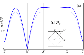
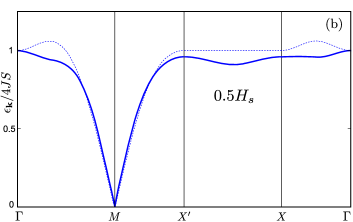
Figure 3: (Color online) Magnon energy of the spin-1/2 square-lattice antiferromagnet below the decay threshold. Dashed lines show the harmonic spin-wave energy $\epsilon_{\bf k}$, solid lines represent the spectrum with the lowest-order quantum correction. The inset in (a) defines the chosen path in the Brillouin zone.

Although, our focus in Sec. IV is on the large-$S$ model, we now present numerical data for the spectrum renormalization (19) in the $S=1/2$ case. Similar results for the other values of spin can be obtained by rescaling quantum corrections in Figs. 3 and 4 by the factor $1/(2S)$. For moderate magnetic fields, $H\lesssim 0.6H_{s}$, the magnitude of the correction to the magnon energy is comparable to that in zero field. Zhitomirsky98b ; Zhitomirsky99 Numerical results for $\bar{\epsilon}_{\bf k}$ along the symmetry directions in the Brillouin zone are shown in Fig. 3 for two values of external field. Contrary to the $H=0$ case, the renormalization is momentum-dependent with increasing deviations from the harmonic theory as the field approaches the decay threshold $H^{*}\approx 0.75H_{s}$. Specifically, there is a sizable dispersion along the magnetic zone boundary $X^{\prime}X$, which further increases in fields above one-half of the saturation field. This is precisely the field regime where the hybridization between one- and two-magnon states grows substantially.

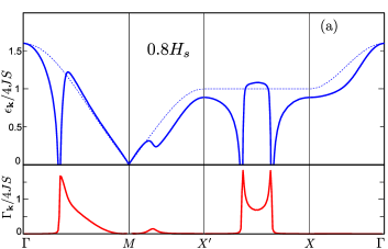
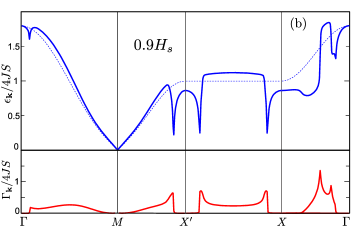
Figure 4: (Color online) Magnon energy and decay rate of the spin-1/2 square-lattice antiferromagnet above the decay threshold. Upper panels: dashed lines show the harmonic spin-wave energy $\epsilon_{\bf k}$, solid lines represent the spectrum with the lowest-order quantum correction $\bar{\epsilon}_{\bf k}$. Lower panels: the decay rate $\Gamma_{\mathbf{k}}$ in the Born approximation.

The lowest-order spin-wave correction changes dramatically at higher fields. The renormalized magnon energy $\bar{\epsilon}_{\bf k}$ exhibits peculiar singularities in the form of jumps and spikes, see Fig. 4. These anomalies signify a breakdown of the perturbative spin-wave expansion since the $1/S$ correction appears to be divergent for certain momenta. Such an outcome is rather surprising because the expansion parameter $\langle a^{\dagger}_{i}a_{i}\rangle/(2S)$ decreases monotonically with the field and vanishes at $H=H_{s}$. In particular, the $1/S$ spin-wave series for the SAFM converges rapidly for the ground-state energy and uniform magnetization,Zhitomirsky98 which agree very well with the numerical results. Luscher09

The observed anomalies in the dynamical properties are clearly related to zero-temperature magnon decays: every singularity in $\bar{\epsilon}_{\bf k}$ is accompanied by a jump or by a peak in the decay rate $\Gamma_{\bf k}$. Zhitomirsky99 ; Chernyshev06 The typical magnitude of $\Gamma_{\bf k}$ for high-energy magnons is comparable to or even exceeds $\epsilon_{\bf k}$, which means that the dynamical response in certain parts of the Brillouin zone is determined predominantly by the two-magnon continuum. A detailed consideration of the origin of the decay anomalies is provided in the next Section, while the asymptotic expressions for $\Gamma_{{\bf k}\to{\bf Q}}$ are derived in Appendix A.

III Kinematics of magnon decays

The problem of spontaneous (zero-temperature) quasiparticle decays generated by cubic anharmonicities has a rather long history. The phenomenon is comprehensively documented for phonons in crystals Klemens67 and for excitations in superfluid ⁴He. Maris77 ; Pitaevskii Similar effects in quantum magnets have started to attract attention only recently. Affleck92 ; Zhitomirsky99 ; Chernyshev06 ; Stone06 ; Masuda06 ; Veillette05 ; Zhitomirsky06 Appearance of spontaneous two-magnon decays for the SAFM is controlled by the energy conservation law:

$$\epsilon_{\bf k}=\epsilon_{\bf q}+\epsilon_{\bf k-q+Q}\ .$$ (21)

The ordering wave-vector $\bf Q$ enters the momentum conservation condition because of the staggered canting of local moments (2). If the energy conservation is satisfied only for a trivial solution ${\bf q}={\bf Q}$, then magnon with the momentum $\bf k$ remains stable. The decay rate $\Gamma_{\bf k}$ becomes finite if there are non-trivial solutions of Eq. (21). A less obvious but not less generic outcome of the mixing between one- and two-particle states is the transfer of some of the Van Hove singularities from the two-particle density of states onto the single-particle spectrum producing various non-analyticities in the latter.Chernyshev06 Thus, studying the kinematics of two-magnon decays for a given dispersion $\epsilon_{\bf k}$ one should consider two related problems: (i) what is the decay region in the momentum space where excitations are unstable, and (ii) where do the renormalization corrections exhibit singular behavior. In the present case, we are also interested in the evolution of both the decay region and the singularities as a function of external magnetic field.

Let us begin with the decay region. At the boundary of such a region the single-magnon branch crosses with the bottom of the two-magnon continuum. Therefore, the boundary can be determined by solving the system of two equations: Eq. (21) and the extremum condition imposed on its r.h.s.:

$${\bf v}_{\bf q}={\bf v}_{\bf k-q+Q}\ ,$$ (22)

where ${\bf v}_{\bf k}=\nabla_{\bf k}\epsilon_{\bf k}$ is a magnon velocity. Generally, one can envisage several types of solutions for the decay threshold: Pitaevskii ; Chernyshev06
(i) decay threshold with the emission of an acoustic magnon $\bf q\rightarrow Q$, determined by the condition

$$|{\bf v}_{\bf k}|=|{\bf v}_{\bf Q}|\equiv c\ ,$$ (23)

(ii) decay threshold with the emission of two magnons with equal momenta ${\bf q}=\frac{1}{2}({\bf k}+{\bf Q})$ found by solving

$$\epsilon_{\bf k}=2\epsilon_{({\bf k}+{\bf Q})/2}\ ,$$ (24)

and (iii) decay threshold with the emission of two nonequivalent magnons found from a direct numerical solution of Eqs. (21) and (22). Then, the decay region is the union of regions obtained for all three decay channels.

Figure 5: (Color online) Field evolution of the decay region of the SAFM in the Born approximation. Numbers correspond to values of $H/H_{s}$.

Magnons in the square-lattice antiferromagnet remain stable up to the threshold field $H^{*}\approx 0.75H_{s}$. Zhitomirsky99 Numerical results for the decay regions in higher magnetic fields are shown in Fig. 5. In fields slightly above $H^{*}$, the instability first affects the acoustic branch producing a cigar-shaped decay region oriented along the $\Gamma M$ diagonal in the Brillouin zone. Expanding energy of the acoustic magnon we obtain

$$\epsilon_{\bf Q+k}\approx ck+\alpha k^{3}\ ,\qquad c=2\sqrt{2}JS\cos\theta\ ,$$

$$\alpha=\frac{c}{16}\Bigl{(}\tan^{2}{\theta}-\frac{9+\cos{4\varphi}}{6}\Bigr{)}\ ,$$ (25)

where $c$ is the acoustic magnon velocity and $\alpha$ is the coefficient of the leading nonlinearity in the dispersion, which depends on the momentum direction via the azimuthal angle $\varphi$. Then, using $\sin{\theta}=H/H_{s}$, one can easily find that $\alpha$ changes its sign from negative in low fields to positive in high fields. Such a change in convexity of the acoustic branch is generally known to result in the kinematic instability with respect to two-particle decays, Maris77 ; Pitaevskii see also discussion in Appendix A. The sign of $\alpha$ changes first for $\varphi=\pi/4$ at the threshold field

$$H^{*}=\frac{2}{\sqrt{7}}\ H_{s}\approx 0.7559\,H_{s}\ .$$ (26)

The above consideration is based on the harmonic expression for $\epsilon_{\bf k}$. Quantum corrections to the magnon dispersion may renormalize the value (26), although the corresponding effect is expected to be small for $S>1/2$.

The described change in the curvature of the Goldstone branch with increasing field is a rather general phenomenon. The acoustic mode changes convexity at the same field (26) in the cubic-lattice Heisenberg antiferromagnet as well as in the stacked square-lattice model for any value of the antiferromagnetic coupling between layers. Moreover, the spin-wave velocity vanishes at $H=H_{s}$ for all Heisenberg antiferromagnets. In this critical field the magnon branch is parabolic at low energies: $\epsilon_{\bf Q+k}\propto k^{2}$. By the continuity argument, the spectrum preserves its positive curvature for a certain range of magnetic fields in the ordered phase, where the asymptotic form (25) holds. This, in turn, implies that the two-particle decays are allowed at least for ${\bf k}\rightarrow{\bf Q}$. A well-known example of such a behavior is provided by the hard-core Bose gas. Beliaev58 More generally, low-energy excitations in the ordered phase near $XY$ quantum critical point are always unstable with respect to two-particle decays. Their decay rate has a universal form $\Gamma_{\bf k}\propto k^{2D-1}$, in agreement with previous results for $D=2$ and 3. Chernyshev06 ; Kreisel08 A more detailed discussion of the decay rate of low-energy magnons in the SAFM is provided in Appendix A.

Magnetic systems with the $O(2)$ rotational symmetry about the field direction belong to the same $XY$ universality class as the Heisenberg SAFM in a field. An analysis of the kinematic conditions for magnon decays in the $XXZ$ square-lattice antiferromagnet in a field parallel to the $\hat{\bf z}$-axis is briefly summarized in Appendix B. Another common example is given by quantum spin systems with the singlet ground state and gapped triplet excitations. The field-induced ordering in such systems has been intensively studied both experimentally Nikuni00 ; Jaime04 ; Regnault06 and theoretically. Affleck91 ; Affleck92 ; Mila98 ; Giamarchi99 The mechanism of spontaneous magnon decays discussed here applies equally to these magnets in the vicinity of the triplet condensation field $H_{c}$ in the ordered phase because of the duality between $H_{c}$ and $H_{s}$. Mila98

For the Heisenberg SAFM, the decay region quickly spreads out across the Brillouin zone as the applied field increases above $H^{*}$ and at $H>0.9H_{s}$ most of the magnons become unstable already in the Born approximation, see Fig. 5. Up to $H\approx 0.85H_{s}$ the boundary of the decay region is entirely determined by the decay into a pair of magnons with equal momenta (24). At higher fields $H\gtrsim 0.85H_{s}$ the decay channel with emission of an acoustic magnon (23) starts to prevail in some parts of the Brillouin zone producing a more complicated shape of the decay region, see Fig. 5.

We now turn to the anomalous features in the magnon spectrum. A close inspection of Fig. 4 reveals two distinct types of singularities in it. The first type is characterized by a dip in $\bar{\epsilon}_{\bf k}$ and by a jump in $\Gamma_{\bf k}$, while the anomaly of the second type consists in a jump in $\bar{\epsilon}_{\bf k}$ accompanied by a peak in $\Gamma_{\bf k}$. The imaginary part of the magnon self-energy is related to the two-magnon density of states via Eq. (20). Hence, in 2D the decay rate $\Gamma_{\bf k}$ exhibits a finite jump upon entering the continuum in accordance with the corresponding Van Hove singularity in the two-particle density of states: Zhitomirsky99

$$\Gamma_{\bf k}\simeq\Theta(\Delta k)\ ,\qquad\textrm{Re}\,\Sigma_{\bf k}(\epsilon_{\bf k})\simeq\ln\frac{\Lambda}{|\Delta k|}\ ,$$ (27)

where $\Lambda$ is a cutoff parameter. The associated singularity in $\textrm{Re}\,\Sigma_{\bf k}(\epsilon_{\bf k})$ follows from the Kramers-Kronig relation.

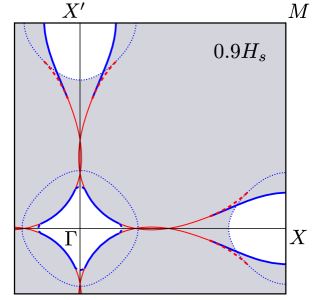
Figure 6: (Color online) Decay region and associated singularities for $H=0.9H_{s}$. Line’s type represents the decay channel: solid is for a pair of magnons with equal momenta, dashed is for a pair of magnons with different momenta, and dotted is for emission of an acoustic magnon. Line’s color indicates the type of singularity in the continuum: blue is for the minimum and red is for the saddle-point.

The second type of anomaly corresponds to an intersection of the one-magnon branch with the saddle-point Van Hove singularity inside the continuum: Chernyshev06

$$\Gamma_{\bf k}\simeq\ln\frac{\Lambda}{|\Delta k|}\ ,\qquad\textrm{Re}\,\Sigma_{\bf k}(\epsilon_{\bf k})\simeq\textrm{sign}(\Delta k)\ .$$ (28)

The boundary line given by Eq. (24) always corresponds to a local extremum and when it enters the interior of the decay region its type changes from a local minimum to a saddle point. The details of such a behavior are illustrated in Fig. 6. Here, solid lines denote singularity contours for the decay into equivalent magnons, dashed lines indicate the decay threshold into a pair of magnons with different momenta, and dotted lines represent the decay threshold for emission of an acoustic magnon. The colors are used to distinguish whether the extremum corresponds to a local minimum (blue) or to a saddle-point (red) in the continuum. The same singularity contour may correspond to a minimum in one part of the Brillouin zone and to a saddle-point in the other. This determines, in turn, whether the logarithmic singularity occurs in the real or imaginary part of the self-energy. Further enhancement of the magnon decay rate may occur in the vicinity of the intersection of two saddle-point lines, an example which can be found in Fig. 6 along the $\Gamma X$ line.

We finish this section with a brief discussion of higher-order magnon decays. Similar to the consideration of the cubic nonlinearities in Sec. II, the quartic terms in Eq. (II), treated beyond the Hartree-Fock approximation, produce decays in the three-particle channel: $b^{\dagger}_{\bf q}b^{\dagger}_{\bf p}b^{\dagger}_{\bf k-q-p}b_{\bf k}$. In addition, higher-order bosonic terms omitted in Sec. II should open decays of one magnon into an arbitrary large number of magnons. Nevertheless, the kinematic analysis above still predicts the correct threshold field for magnon decays. This is because all higher-order $n$-particle decays with $n\geq 3$ are energetically forbidden if no two-magnon decays are allowed in the whole Brillouin zone. Harris71 In our case, this means that magnons in the SAFM remain completely stable up to the two-magnon threshold field $H^{*}$. Once two-magnon decays become possible at $H>H^{*}$, the $n$-magnon decays are also kinematically allowed. Generally, we expect the corresponding decay rates to be significantly smaller than for the two-magnon decays because of their higher $1/S$ order. Moreover, the multi-magnon decays should not produce any singularities of the type (27) and (28) due to higher-dimensional integration in corresponding analogs of Eq. (20).

IV Self-consistent theory of magnon decays

IV.1 One-magnon Green’s function

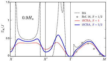
Figure 7: (Color online) Magnon decay rate $\Gamma_{\mathbf{k}}$ at $H=0.9H_{s}$ calculated in the Born approximation (dashed line) and in the iSCBA scheme for $S=1$ (thin solid line, red) and for $S=5/2$ (bold solid line, blue). Dots in $\Gamma M$ panel are $-{\rm Im}\Sigma_{\bf k}(\bar{\epsilon}_{\bf k})$ for $S=1/2$ from Ref. Zhitomirsky99, .

Figure 8: (Color online) Intensity maps of the magnon decay rate $\Gamma_{\mathbf{k}}$ calculated within the iSCBA for several values of external magnetic field and for the two values of the spin: $S=1$ (upper panels) and $S=5/2$ (lower panels).

Singular quantum corrections to the magnon spectrum obtained in the leading $1/S$ order are generally regularized by higher-order processes. Details of such a regularization depend on the specific shape of $\epsilon_{\bf k}$. An important aspect of the kinematics of the field-induced decays in SAFM is that the low-energy magnons created in a decay process are unstable by themselves. Qualitatively, the inverse life-time $\Gamma_{\bf q}$ of the decay products cuts off the singularities in (27) and (28) by changing

$$|\Delta k|\rightarrow\sqrt{(\Delta k)^{2}+(\Gamma_{\bf q}/c_{\bf q})^{2}}\ ,$$

where $c_{\bf q}$ can be expressed through the velocities of the decay products. Accordingly, the self-consistent procedure, which replaces the bare magnon Green’s functions in the self-energy diagrams in Fig. 2 with the renormalized ones, should produce non-singular quantum corrections. The main problem with such a self-consistent Born approximation (SCBA) is that it opens an unphysical gap for acoustic magnons in violation of the Goldstone theorem. Here we avoid this problem by performing a restricted self-consistent calculation, which takes into account the imaginary part of the magnon self-energy and neglects the real part of it. Such an approximation, which is referred to as iSCBA in the following, is expected to yield reasonable accuracy for spins $S\geq 1$. Indeed, in the low-field region the nonsingular quantum corrections to the magnon energy do not exceed 15–18% in the case of $S=1/2$, see Sec. II. For larger spins this correction is further reduced by a factor $1/(2S)$ and already for $S\gtrsim 1$ it corresponds only to a small shift of the magnon energy.

In the simplest realization of the iSCBA we further neglect the frequency dependence of $\textrm{Im}\,\Sigma_{\bf k}(\omega)$ and impose the following form of the one-magnon Green’s function:

$$G^{-1}({\bf k},\omega)=\omega-\epsilon_{\bf k}+i\Gamma_{\bf k}\ .$$ (29)

The magnon decay rate $\Gamma_{\bf k}$ is calculated self-consistently from

$$\Gamma_{\bf k}=-\textrm{Im}\,\Sigma({\bf k},\epsilon_{\bf k})\ ,$$ (30)

with $\Sigma({\bf k},\epsilon_{\bf k})$ from Fig. 2. Physically, the approximation (29) amounts to assuming the Lorentzian shape of the quasiparticle peak in the dynamical response. Such a self-consistent scheme has been previously applied to the problem of phonon broadening in superfluid heliumSluckin74 and in quasicrystals.Kats05 In the present case, with two types of cubic vertices the self-consistent equation on $\Gamma_{\bf k}$ becomes

$$\Gamma_{\bf k} = \frac{1}{2}\sum_{\bf q}\biggl{[}\frac{|\Phi_{1}({\bf k},{\bf q})|^{2}(\Gamma_{\bf q}+\Gamma_{\bf k-q+Q})}{(\epsilon_{\bf k}-\epsilon_{\bf q}-\epsilon_{\bf k-q+Q})^{2}+(\Gamma_{\bf q}+\Gamma_{\bf k-q+Q})^{2}}$$ (31)

$$+ \frac{|\Phi_{2}({\bf k},{\bf q})|^{2}(\Gamma_{\bf q}+\Gamma_{\bf k+q-Q})}{(\epsilon_{\bf k}+\epsilon_{\bf q}+\epsilon_{\bf k+q-Q})^{2}+(\Gamma_{\bf q}+\Gamma_{\bf k+q-Q})^{2}}\biggr{]}.$$

One important consequence of the self-consistent consideration is that spontaneous decays are not restricted to the decay region in Fig. 5, defined in the Born approximation. Since the finite decay rate of magnons inside the decay region means an uncertainty in their energy, the energy conservation condition (21) is relaxed and magnons just outside the decay region are also allowed to decay. Therefore, the decay threshold boundary is smeared and the decay probability disappears gradually rather than in a step-like fashion.

Numerical solutions of Eq. (31) have been obtained iteratively using two different grids in the momentum space: a sparse mesh for the momentum $\bf k$ of $40\times 40$ points in the full Brillouin zone and a much tighter grid for integration over the momentum $\bf q$ with up to $1000\times 1000$ points. The values of $\Gamma_{\bf q}$ for the integrand were obtained from $\Gamma_{\bf k}$ by a bicubic interpolation. To improve convergence at low energies we also impose the asymptotic form $\Gamma_{\bf Q+k}\sim k^{3}$ for small $k$, see Appendix A. Sufficient accuracy is typically achieved after 5–8 iteration steps. Note, that the second term on the r.h.s. of Eq. (31) from the source diagram in Fig. 2 is always small and can be safely neglected.

Figure 7 compares $\Gamma_{\bf k}$ obtained in the Born approximation with the iSCBA results for $S=1$ and $S=5/2$ at $H=0.9H_{s}$. One can see that the singular behavior of $\Gamma_{\bf k}$ near the Van Hove singularities is completely removed in the self-consistent calculation. The typical amplitude of the decay rate in Fig. 7 away from $\Gamma$ and $M$ points is $\Gamma_{\bf k}\lesssim 0.5J$, which should be compared with the typical magnon energies $\epsilon_{\bf k}\sim 4JS$. Another notable aspect of the self-consistent regularization is in the spin-dependence of the decay rate: $\Gamma_{\bf k}$ is larger for larger spins in most of the Brillouin zone. Such a dependence should not be confused with the relative strength of the spectrum broadening $\Gamma_{\bf k}/\epsilon_{\bf k}\sim\Gamma_{\bf k}/JS$, which is still larger for smaller values of the spin. The decay rate approaches the spin-independent Born result $\Gamma^{(0)}_{\bf k}$ only in the limit $S\to\infty$. In particular, while $\Gamma_{\bf k}\simeq\Gamma^{(0)}_{\bf k}+O(1/S)$ away from the singular points, one finds $\Gamma_{\bf k}\sim\ln S$ in their vicinity.Chernyshev06

Further details on the momentum distribution of the magnon decay rate in different fields are provided in the form of intensity maps for $\Gamma_{\bf k}/4JS$ in Fig. 8. Comparison of the upper ($S=1$) and the lower ($S=5/2$) row reveals similar patterns in the momentum distribution of $\Gamma_{\bf k}$ for these two values of spin. The intensity of the decays in Fig. 8 is determined by either the volume of the decays or by the proximity to the Van Hove singularities of the two-magnon continuum. Specifically, in the lower fields $H\lesssim 0.9H_{s}$ the magnon damping is most significant in the broad region around $(\pi/2,\pi/2)$ point. This is a consequence of the large phase space volume for the two-particle decays in this region. In higher fields the maximums in the decay rate shift towards the $\Gamma X$ and $\Gamma X^{\prime}$ lines. The enhancement of $\Gamma_{\bf k}$ here is due to an intersection of the two singularity lines discussed in Sec. III. Overall, the maximum magnon decay rate in all fields does not exceed $\Gamma^{\rm max}_{\bf k}\sim 0.7$–$0.8J$. Thus, we may conclude that the spin waves in large-$S$ quantum antiferromagnets above the decay threshold $H^{*}$ are damped but still well-defined quasiparticles.

The above conclusion seems to be at odds with the behavior of the spin-1/2 SAFM. In this case, magnons were shown to be overdamped in most of the Brillouin zone by both the spin-wave calculation, which used a different version of the SCBA, Zhitomirsky99 and by the numerical QMC simulations.Olav08 Such a difference in the effect of magnon interaction between $S=1/2$ and $S\geq 1$ models deserves a separate discussion. We compare directly the imaginary part of the magnon self-energy at the quasiparticle pole, $-{\rm Im}\Sigma_{\bf k}(\bar{\epsilon}_{\bf k})$, for the $S=1/2$ case obtained in Ref. Zhitomirsky99, with $\Gamma_{\bf k}$ found in this work, see the data points along $\Gamma M$ direction in Fig. 7. One can see that $S=1/2$ and $S\geq 1$ results are quantitatively close. Naively, this would mean that quasiparticles in the $S=1/2$ antiferromagnet should also be reasonably well-defined. However, this consideration neglects the spectral weight redistribution. The analytical calculation Zhitomirsky99 and the QMC study Olav08 have shown a significant non-Lorentzian broadening of the spectral lines, which takes the form of a double-peak structure in the dynamical susceptibility. Therefore, the overdamping in the $S=1/2$ case is produced by two effects: broadening of the quasiparticle peak and spectral weight redistribution. Note, that the latter effect was completely excluded in the recent hard-core boson study,Syromyat09 which explicitly neglected the frequency dependence of the magnon self-energy. Such an approximation may have lead Ref. Syromyat09, to the conclusion of only weak-to-moderate damping of spin excitation in the $S=1/2$ SAFM in a field, in contrast with Refs. Zhitomirsky99, and Olav08, .

Since the iSCBA developed here also neglects the spectral weight redistribution, one can question its validity on the same grounds. To verify the validity of this approach we have checked the accuracy of the Lorentzian approximation used in (29) by keeping the full frequency dependence of $\textrm{Im}\,\Sigma_{\bf k}(\omega)$ and by utilizing general representation for the magnon Green’s function

$$G({\bf k},\omega)=\int_{-\infty}^{\infty}\textrm{d}x\,\frac{A_{\bf k}(x)}{\omega-x+i0}\ .$$ (32)

The self-consistent equation is formulated for the spectral function $A_{\bf k}(\omega)$ excluding again the real part of the magnon self-energy. Numerical results (not shown) exhibit only a small asymmetry of magnon peaks and only for the lowest $S=1$ case. This justifies the use of the frequency-independent iSCBA scheme for $S\geq 1$ antiferromagnets and confirms the perturbative role of damping for them once the singularities are regularized by a self-consistent calculation.

IV.2 Dynamical structure factor

The inelastic neutron scattering experiments probe the spin-spin correlation function

$$\mathcal{S}^{\alpha\beta}({\bf k},\omega)=\int_{-\infty}^{\infty}\frac{\mbox{d}t}{2\pi}\,\langle S^{\alpha}_{\bf k}(t)S^{\beta}_{-\bf k}\rangle\,e^{i\omega t}$$ (33)

defined in the global laboratory frame, while the spin-wave calculations are conveniently performed in the local rotating frame, see Sec. II. First, we relate these two forms of the correlation function with the help of Eq. (2):

$$\mathcal{S}^{x_{0}x_{0}}({\bf k},\omega) = \sin^{2}\!\theta\,\mathcal{S}^{xx}({\bf k},\omega)+\cos^{2}\!\theta\,\mathcal{S}^{zz}({\bf k}-{\bf Q},\omega)\,,$$

$$\mathcal{S}^{z_{0}z_{0}}({\bf k},\omega) = \cos^{2}\!\theta\,\mathcal{S}^{xx}({\bf k}-{\bf Q},\omega)+\sin^{2}\!\theta\,\mathcal{S}^{zz}({\bf k},\omega)\,,$$

$$\mathcal{S}^{y_{0}y_{0}}({\bf k},\omega) = \mathcal{S}^{yy}({\bf k},\omega)\ .$$ (34)

Here we have omitted the cross-terms $(\alpha\neq\beta)$ on the r.h.s., which can be shown to be small numerically. Second, we relate the dynamical structure factor (34) to the time-ordered spin Green’s function $\mathcal{G}^{\alpha\beta}({\bf k},t)=-i\langle TS^{\alpha}_{\bf k}(t)S^{\beta}_{-\bf k}\rangle$ using the fluctuation-dissipation theorem at zero temperature:

$$\mathcal{S^{\alpha\beta}}({\bf k,\omega})=-\frac{1}{\pi}\,\mbox{Im}\,\mathcal{G}^{\alpha\beta}({\bf k},\omega)\ .$$ (35)

Finally, we express spin operators via the Holstein-Primakoff bosons and, after some of algebra, obtain the following expressions

$$S^{xx}({\bf k},\omega) = -S\Lambda_{+}\>(u_{\bf k}+v_{\bf k})^{2}\;\mbox{Im}\,G({\bf k,\omega})\ ,$$

$$S^{yy}({\bf k},\omega) = -S\Lambda_{-}\>(u_{\bf k}-v_{\bf k})^{2}\;\mbox{Im}\,G({\bf k,\omega})\ ,$$ (36)

$$S^{zz}({\bf k},\omega) = -\frac{1}{N}\displaystyle{\sum_{\bf q}}\,(u_{\bf k-q}v_{\bf q}\!+\!u_{\bf q}v_{\bf k-q})^{2}$$

$$\times\,\mbox{Im}\,\left\{\int_{-\infty}^{\infty}\mbox{d}x\;G({\bf q},x)\,G({\bf k}-{\bf q},\omega-x)\right\}\,.$$

Here $\Lambda_{\pm}=1-(2n\pm\delta)/2S$ are the Hartree-Fock spin reduction factors and $G({\bf k},\omega)$ is the magnon Green’s function from (29).

In the equation above, spin fluctuations are separated into transverse ($xx$, $yy$) and longitudinal ($zz$) components relative to the local spin direction, which correspond to scattering from states with odd and even number of magnons, respectively.Canali93 An important effect of the spin canting on the dynamical structure factor is the redistribution of the spectral weight over the two well-separated transverse modes,Heilmann81 which overlap only at the magnetic zone boundary. As a result, Eq. (34) contains a mixture of two transverse contributions at momenta ${\bf k}$ and ${\bf k-Q}$. The first mode corresponds to spin fluctuations perpendicular to the magnetic field direction (in-plane mode), while the second mode, shifted by the ordering wave-vector $\bf{Q}$, corresponds to the fluctuations along the field direction (out-of-plane mode). In strong magnetic fields the in-plane mode is enhanced and dominates over the out-of-plane fluctuations, which gradually disappear as $H\rightarrow H_{s}$. Note also the existence of two distinct longitudinal multimagnon continua associated with each of the transverse branches.

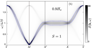
Figure 9: (Color online) Transverse part of the dynamical structure factor (gray scale) computed using the iSCBA for $S=1$ and for the two values of external magnetic field. Dashed lines (blue) enclose the region $\epsilon_{\bf k}\pm\Gamma_{\bf k}$ corresponding to the full-width at half maximum of the corresponding quasiparticle peaks.

Results summarized in Eqs. (34) and (36) are quite general and can be adapted to a variety of specific experimental situations. As a particular example, the dynamical structure factor accessible to unpolarized neutron scattering experiment with a vertical magnetic field reads as $\mathcal{S}({\bf k},\omega)=\mathcal{S}_{\perp}({\bf k},\omega)+\mathcal{S}^{z_{0}z_{0}}({\bf k},\omega)$. The explicit expression for $\mathcal{S}_{\perp}({\bf k},\omega)$ depends on the experimental details via a momentum-dependent polarization factor. In the following, such a factor is deliberately ignored and the expression $\mathcal{S}({\bf k},\omega)=\mathcal{S}^{x_{0}x_{0}}+\mathcal{S}^{y_{0}y_{0}}+\mathcal{S}^{z_{0}z_{0}}$ is used for an illustration. The combined $\mathcal{S}({\bf k},\omega)$ computed using the self-consistent magnon Green’s function obtained in previous subsection is shown for $S=1$ and $S=5/2$ antiferromagnets in Figs. 9 and 10, respectively. One can clearly see the presence of two transverse modes with the more intense in-plane and the weaker out-of-plane mode.

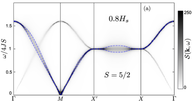
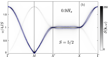
Figure 10: (Color online) Same as Fig. 9 for $S=5/2$.

A distinct fingerprint of spontaneous magnon decays as compared to other possible damping mechanisms is their characteristic dependence on the momentum and on the applied magnetic field. In the field range $H^{*}\leq H\leq 0.9H_{s}$ the magnon damping is most significant along the magnetic zone boundary $X^{\prime}X$ with the maximum at $(\pi/2,\pi/2)$. In higher magnetic fields $H\geq 0.9H_{s}$ the strongest damping occurs along the $\Gamma X$ line, where the singularity-enhanced decays are most pronounced. Our predictions for the former field regime are in a qualitative agreement with the very recent inelastic neutron scattering results of Masuda et al.Masuda10   for the spin-5/2 layered square-lattice antiferromagnet Ba₂MnGe₂O₇. However, the largest magnon linewidth measured experimentally exceeds our theoretical estimate $2\Gamma_{\bf k}\simeq 1.5J$ for $H=0.82H_{s}$ by a factor of 2–3. The larger experimental linewidth may be related to the overlap of the two transverse modes along the magnetic zone boundary. Therefore, we propose that the inelastic neutron scattering measurements at $H\geq 0.9H_{s}$ in the vicinity of $(\pi/2,0)$ point where the two transverse modes are well separated may provide a benchmark for the field-induced spontaneous magnon decays in the SAFM.

V Conclusions

We have presented a detailed analysis of the field-induced decay dynamics in the square-lattice antiferromagnet within the framework of the spin-wave theory. In magnetic fields exceeding the threshold field for two-particle decays, the $1/S$ quantum correction to the magnon spectrum exhibits singularities for certain momenta. These are related either to the decay thresholds Zhitomirsky99 or to the saddle-point Van Hove singularities in the two-magnon continuum.Chernyshev06 Such singularities invalidate the usual $1/S$-expansion because the resultant renormalized spectrum contains divergences. The encountered problem is rather generic and must be common to a variety of 2D models regardless of the on-site spin value. For the systems with large spins the situation is especially aggravating as the $1/S$ expansion turns from a reliable approach to the one producing unphysical divergences, which complicate any sensible comparison with experimental or numerical data.

In the present work we have developed a self-consistent regularization scheme, which is applicable to a variety of problems in the decay dynamics of large-$S$ quantum antiferromagnets. The self-consistently calculated damping in the SAFM is free from singularities and gives an upper limit on the decay rate: $(\Gamma_{\bf k}/\epsilon_{\bf k})\lesssim 0.2/S$. Overall, spin-waves in the SAFM with $S\geq 1$ in magnetic field $H>H^{*}$ do acquire finite broadening, but remain well-defined quasiparticles. The regularized singularities also lead to a parametric enhancement of the magnon damping and produce a distinct field- and momentum-dependence of $\Gamma_{\bf k}$, which is illustrated for the $S=1$ and $S=5/2$ in Figs. 7-10. These results can be used for quantitative comparison in future experimental studies of the field-induced spontaneous magnon decays.

For the spin-1/2 SAFM the situation appears to be somewhat more delicate. Previous analyticalZhitomirsky99 and numericalOlav08 studies have predicted overdamped one-magnon excitations in a large part of the Brillouin zone. The SCBA scheme used in Ref. Zhitomirsky99, includes a self-consistent renormalization of only one inner magnon line in the decay diagram of Fig. 2 and is, in a sense, not as consistent as the present approach. On the other hand, that approach does take into account the real part of the spectrum renormalization and, as a consequence, the quasiparticle weight redistribution. Such an effect can be deemed small for larger spins, but it is more important for $S=1/2$ and is likely to contribute to further enhancement of the damping in this case. Since the imaginary part of the self-energy at the quasiparticle pole for $S=1/2$ in Ref. Zhitomirsky99, correlates closely with the iSCBA results of the present work (Fig. 7), we believe that this is the correct explanation of the differences between $S=1/2$ and $S\geq 1$ cases. There are also qualitative and quantitative similarities of the analytical Zhitomirsky99 and numerical results, Olav08 in particular the double-peak structure in the spectral function. While the QMC approach may involve its own uncertainties due to numerical interpolation from imaginary to real frequencies,Olav08 such a correspondence between results of two very different methods is encouraging. Further theoretical efforts may be needed to clarify completely the detailed behavior of the dynamical structure factor for the spin-1/2 SAFM. Finally, performing inelastic neutron scattering measurements on suitable spin-1/2 compounds would also be important.

Appendix A Decay of low-energy magnons

In the case of the Heisenberg SAFM and other two-sublattice antiferromagnets in applied magnetic field the low-energy spectrum consists of the single weakly nonlinear acoustic branch (25). In the following consideration all momenta are taken relative to the magnetic ordering wave-vector $\bf Q$: $\epsilon_{\bf Q+k}\rightarrow\epsilon_{\bf k}\approx ck+\alpha k^{3}$. First, we verify explicitly the energy conservation condition for the two-particle decays (21). If the nonlinearity of the spectrum is weak $\alpha k^{3}\ll ck$, the two magnons emitted in a spontaneous decay process have their momenta $\bf q$ and ${\bf q}^{\prime}={\bf k}-{\bf q}$ almost parallel to the direction of $\bf k$. Then,

$$|{\bf k}-{\bf q}|\approx k-q+\frac{kq\varphi^{2}}{2(k-q)}\ ,$$ (37)

where $\varphi$ is a small angle between $\bf q$ and $\bf k$, and the energy conservation can be written as

$$\epsilon_{\bf k}-\epsilon_{\bf q}-\epsilon_{\bf k-q}\approx 3\alpha kq(k-q)-\frac{ckq\varphi^{2}}{2(k-q)}$$ (38)

$$\mbox{}\quad=-\frac{ckq}{2(k-q)}\left(\varphi^{2}-\varphi_{0}^{2}\right)\ ,\quad\varphi_{0}^{2}=\frac{6\alpha}{c}(k-q)^{2}\ .$$

One can see that the nontrivial solution $\varphi=\varphi_{0}$ exists only for the positive sign of the cubic nonlinearity $\alpha$.Maris77 ; Pitaevskii

Next, we derive the asymptotic, $k,q\rightarrow 0$ form for the decay vertex $\tilde{\Phi}_{1}({\bf k},{\bf q})$, see Eq. (14). In order to obtain the correct expression one needs to retain three leading terms in the expansion of the Bogolyubov coefficients $u_{\bf k}$ and $v_{\bf k}$ in small $k$. This yields

$$\tilde{\Phi}_{1} \approx -\left(\frac{\cos\theta}{\sqrt{2}}\right)^{1/2}\;\left[\frac{q+|{\bf k}-{\bf q}|-k}{\sqrt{kq(k-q)}}+\lambda\sqrt{kq(k-q)}\right]\ ,$$ (39)

$$\lambda=\frac{3}{4\cos^{2}\theta}-\frac{3\alpha}{c}\ .$$

For momenta $\bf k$ and $\bf q$, which satisfy the energy conservation condition (21), the decay vertex further simplifies into

$$\tilde{\Phi}_{1}({\bf k},{\bf q})\approx-\frac{3}{4\cos^{2}\theta}\,\left(\frac{\cos\theta}{\sqrt{2}}\right)^{1/2}\,\sqrt{kq(k-q)}\ .$$ (40)

Substituting (38) and (40) into the Born expression for the decay rate in Eq. (20) one obtains

$$\Gamma_{\bf k}=\frac{3J}{16\pi}\,\tan^{2}\!\theta\;\sqrt{\frac{c}{6\alpha}}\;k^{3}\ .$$ (41)

The bare values of $c$ and $\alpha$ are given by Eq. (25), although one may generally use renormalized parameters. Note, that the asymptotic expression (41) differs from the result provided in Ref. Kreisel08, . Therefore, we have verified that our expression for $\Gamma_{\bf k}$ in (41) agrees with the direct numerical integration of Eq. (20) in the limit of small $k$.

As $H\to H_{s}$, the velocity of the acoustic mode decreases and the condition of a weak nonlinearity applies to a progressively narrower range of momenta $k^{2}\ll 8\cos^{2}\theta$ reducing the range of validity of the asymptotic expression (41). Outside that domain one can use the parabolic form of the magnon dispersion $\epsilon_{\bf k}\approx JSk^{2}$ to derive another useful asymptotic expression for the decay rate. In this regime $u_{\bf k}\approx 1$ and $v_{\bf k}=O(\cos\theta)\approx 0$ and the decay vertex becomes $\tilde{\Phi}_{1}({\bf k},{\bf q})\approx-2$. The angle between the emitted and the initial magnon can now be large: $\cos\varphi_{0}=q/k$. Performing an analytical integration in Eq. (20) and taking into account that $\cos^{2}\theta\approx 2(1-H/H_{s})$ we obtains

$$\Gamma_{\bf k}\approx 16\left(1-\frac{H}{H_{s}}\right)\ ,$$ (42)

which is valid for $4\sqrt{1-H/H_{s}}\ll k\ll 1$.

Modifications to the asymptotic expression (41) are also expected in the field regime just above the decay threshold field, $H\rightarrow H^{*}$. In this case, $\alpha\to 0$ and the coefficient in front of $k^{3}$ in the Born expression for $\Gamma_{\bf k}$ in (41) diverges. Such a nonanalytic behavior is nothing but the long-wavelength version of the decay threshold singularities. The self-consistent regularization (31) of Sec. IV should remain applicable in this limit. In order to verify that the power-law behavior (41) is not modified within the SCBA we substitute a general power-law ansatz for the decay rate $\Gamma_{\bf k}=\beta k^{n}$ and assume that the damping is much larger than the nonlinearity but still much smaller than the magnon energy: $\alpha k^{3}\ll\beta k^{n}\ll ck$. In this case, the decay angle is scaled as $\varphi^{2}\sim k^{n-1}$ with $q\sim k$, which makes the decay vertex $\tilde{\Phi}_{1}({\bf k},{\bf q})\sim k^{n-3/2}$ instead of (40). The power counting on both sides of Eq. (31) yields a unique solution: $n=3$. Therefore, the Born exponent $\Gamma_{\bf k}=\beta k^{3}$ is not changed by the self-consistent procedure. The damping coefficient $\beta$ does not diverge near the decay threshold field anymore because $\alpha$ drops out from the self-consistent equation on $\Gamma_{\bf k}$. Instead, $\beta$ exhibits a step-like behavior in $(H-H^{*})$, which is in an accord with the 2D character of the Van Hove singularity at the border of the two-particle continuum.

Appendix B Decays in $XXZ$ SAFM

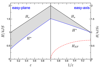
Figure 11: (Color online) Phase diagram of the XXZ model in applied field as a function of anisotropy parameter $\varepsilon$. The field range where spontaneous magnon decays are allowed is shown in gray.

The Hamiltonian of the $XXZ$ antiferromagnet on a square-lattice is

$$\hat{\cal H}=J\sum_{\langle ij\rangle}\left[S_{i}^{\perp}S_{j}^{\perp}+\varepsilon S_{i}^{z}S_{j}^{z}\right]-H\sum_{i}S_{i}^{z}\ .$$ (43)

The values of the anisotropy parameter $0\leq\varepsilon<1$ describe the spin system with the easy-plane anisotropy, whereas $\varepsilon>1$ corresponds to the easy-axis case.

Minimization of the classical energy yields the transition field into a fully saturated state

$$H_{s}=4JS(1+\varepsilon)\ .$$ (44)

For the easy-axis case, the spin-flop transition between the collinear state and the canted antiferromagnetic state takes place at

$$H_{SF}=2JS\sqrt{2(\varepsilon^{2}-1)}\ .$$ (45)

The harmonic spectrum in the canted antiferromagnetic state is given by the same expression Eq. (6) as for the Heisenberg SAFM with the substitution $\cos 2\theta\rightarrow(\varepsilon\cos^{2}\theta-\sin^{2}\theta)$. Performing the same type of kinematic analysis as in Sec. III, we find that the curvature of the acoustic branch changes at the threshold field

$$H^{*}=4JS\sqrt{(1+\varepsilon)\Bigl{(}\frac{1}{7}+\varepsilon\Bigr{)}}\ .$$ (46)

Above this field spontaneous two-magnon decays are kinematically allowed. The phase diagram in the $H$–$\varepsilon$ plane is summarized in Fig. 11. Note, that in the right panel the units of the field are different from the left panel.

Several observations are in order: (i) for arbitrary $\varepsilon$ there is a finite range of fields below the saturation field where magnons are unstable; (ii) the spin-flop field $H_{SF}$ in the easy-axis regime is always below the decay threshold field $H^{*}$; (iii) the easy-plane anisotropy pushes the decay instability to lower fields compared to the isotropic model. In the $XY$-limit ($\varepsilon=0$) the ratio $H^{*}/H_{s}=1/\sqrt{7}\approx 0.38$ is two times smaller than for the Heisenberg antiferromagnet. This might be important for the search of experimental systems where the phenomenon of magnon decays can be observed. Note also that the easy-plane anisotropy appears naturally in the mapping of the BEC-type transition of the triplet excitations in quantum magnets with the singlet ground state onto the saturation field transition of an effective pseudo-spin-1/2 model.Mila98 The typical value of the anisotropy parameter in these problems is $\varepsilon=0.5$, which implies that spontaneous magnon decays must exist in an extended interval of fields above the condensation field $H_{c}$.

References

- (1) E. Manousakis, Rev. Mod. Phys. 63, 1 (1991).
- (2) F. M. Woodward, A. S. Albrecht, C. M. Wynn, C. P. Landee, and M. M. Turnbull, Phys. Rev. B 65, 144412 (2002).
- (3) T. Lancaster, S. J. Blundell, M. L. Brooks, P. J. Baker, F. L. Pratt, J. L. Manson, M. M. Conner, F. Xiao, C. P. Landee, F. A. Chaves, S. Soriano, M. A. Novak, T. P. Papageorgiou, A. D. Bianchi, T. Herrmannsdorfer, J. Wosnitza, and J. A. Schlueter, Phys. Rev. B 75, 094421 (2007).
- (4) F. C. Coomer, V. Bondah-Jagalu, K. J. Grant, A. Harrison, G. J. McIntyre, H. M. Ronnow, R. Feyerherm, T. Wand, and M. Meissner, D. Visser, and D. F. McMorrow, Phys. Rev. B 75, 094424 (2007).
- (5) N. Tsyrulin, T. Pardini, R. R. P. Singh, F. Xiao, P. Link, A. Schneidewind, A. Hiess, C. P. Landee, M. M. Turnbull, and M. Kenzelmann, Phys. Rev. Lett. 102, 197201 (2009).
- (6) R. Coldea, D. A. Tennant, K. Habicht, P. Smeibidl, C. Wolters, and Z. Tylczynski, Phys. Rev. Lett. 88, 137203 (2002).
- (7) S. Nakatsuji, Y. Nambu, H. Tonomura, O. Sakai, S. Jonas, C. Broholm, H. Tsunetsugu, Y. M. Qiu, and Y. Maeno, Science 309, 1697 (2005).
- (8) I. Affleck, Phys. Rev. B 43, 3215 (1991).
- (9) I. Affleck and G. F. Wellman, Phys. Rev. B 46, 8934 (1992).
- (10) F. Mila, Eur. Phys. J. B 6, 201 (1998).
- (11) T. Giamarchi and A. M. Tsvelik, Phys. Rev. B 59, 11398 (1999).
- (12) T. Nikuni, M. Oshikawa, A. Oosawa, and H. Tanaka, Phys. Rev. Lett. 84, 5868 (2000).
- (13) M. Jaime, V. F. Correa, N. Harrison, C. D. Batista, N. Kawashima, Y. Kazuma, G. A. Jorge, R. Stein, I. Heinmaa, S. A. Zvyagin, Y. Sasago, and K. Uchinokura, Phys. Rev. Lett. 93, 087203 (2004).
- (14) L. P. Regnault, A. Zheludev, M. Hagiwara, A. Stunault, Phys. Rev. B 73, 174431 (2006).
- (15) M. E. Zhitomirsky and T. Nikuni, Phys. Rev. B 57, 5013 (1998).
- (16) M. E. Zhitomirsky and A. L. Chernyshev, Phys. Rev. Lett. 82, 4536 (1999).
- (17) O. F. Syljuasen, Phys. Rev. B 78, 180413(R) (2008).
- (18) A. Lüscher and A. M. Läuchli, Phys. Rev. B 79, 195102 (2009).
- (19) A. Kreisel, F. Sauli, N. Hasselmann, and P. Kopietz, Phys. Rev. B 78, 035127 (2008).
- (20) A. V. Syromyatnikov, Phys. Rev. B 79, 054413 (2009).
- (21) A. L. Chernyshev and M. E. Zhitomirsky, Phys. Rev. B 79, 174402 (2009).
- (22) C. J. Hamer, Z. Weihong, and P. Arndt, Phys. Rev. B 46, 6276 (1992).
- (23) J. I. Igarashi, Phys. Rev. B 46, 10763 (1992).
- (24) C. M. Canali and M. Wallin, Phys. Rev. B 48, 3264 (1993).
- (25) J. I. Igarashi and T. Nagao Phys. Rev. B 72, 014403 (2005).
- (26) A. L. Chernyshev and M. E. Zhitomirsky, Phys. Rev. Lett. 97, 207202 (2006); Phys. Rev. B 79, 144416 (2009).
- (27) T. Holstein and H. Primakoff, Phys. Rev. 58, 1098 (1940).
- (28) T. Oguchi, Phys. Rev. 117, 117 (1960).
- (29) M. E. Zhitomirsky and T. Nikuini, Physica B 241–243, 573 (1998).
- (30) P. G. Klemens, J. Appl. Phys. 38, 4573 (1967).
- (31) H. J. Maris, Rev. Mod. Phys. 49, 341 (1977).
- (32) E. M. Lifshitz and L. P. Pitaevskii, Statistical Physics II (Pergamon, Oxford, 1980).
- (33) M. Y. Veillette, A. J. A. James, and F. H. L. Essler, Phys. Rev. B 72, 134429 (2005).
- (34) M. B. Stone, I. A. Zaliznyak, T. Hong, C. L. Broholm, and D. H. Reich, Nature 440, 187 (2006).
- (35) T. Masuda, A. Zheludev, H. Manaka, L.-P. Regnault, J.-H. Chung, and Y. Qiu, Phys. Rev. Lett. 96, 047210 (2006).
- (36) M. E. Zhitomirsky, Phys. Rev. B 73, 100404(R) (2006).
- (37) S. T. Beliaev, Zh. Eksp. Teor. Fiz. 34, 433 (1958) [Sov. Phys. JETP 7, 299 (1958)].
- (38) A. B. Harris, D. Kumar, B. I. Halperin, and P. C. Hohenberg, Phys. Rev. B 3, 961 (1971).
- (39) T. J. Sluckin and R. M. Bowley, J. Phys. C 7, 1779 (1974).
- (40) E. I. Kats and A. R. Muratov, J. Phys. Condens. Mat. 17, 6849 (2005).
- (41) I. U. Heilmann, J. K. Kjems, Y. Endoh, G. F. Reiter, G. Shirane, and R. J. Birgeneau, Phys. Rev. B 24, 3939 (1981).
- (42) T. Masuda, S. Kitaoka, S. Takamizawa, N. Metoki, K. Kaneko, K. C. Rule, K. Kiefer, H. Manaka, and H. Nojiri, Phys. Rev. B 81, 100402(R) (2010).