Hysteresis of atmospheric parameters of 12 RR Lyrae stars
based on multichannel simultaneous Strömgren photometry

Abstract

Aims. RR Lyrae stars have been observed to improve the insight into the processes at work in their atmospheres.

Methods. Simultaneous Strömgren-photometry allows to obtain a rapid sequence of measurements in which photometric indices are unaffected by non-optimum observing conditions. The indices $y$, $b-y$, and $c_{1}$ are used with an established calibration to derive $T_{\rm eff}$ and to derive the gravity, $\log g_{\rm BJ}$ from the Balmer jump, throughout the pulsation cycle. By employing the equations for stellar structure, additional parameters can be derived.

Results. Strömgren photometry and its calibration in terms of $T_{\rm eff}$ and $\log g$ can be used to determine the run of $R$ and the atmosphere pulsation velocity. We find that the Balmer-line strengths are correlated with $T_{\rm eff}$ and that the strength of the Ca ii K line correlates well with the radius of the star and thus the pulsation-dependent density of the atmosphere. The density in the stellar atmosphere fluctuates as indicated by the changes in the gravity $\log g_{\rm BJ}$, derived from $c_{1}$, between 2.3 and 4.5 dex. Also the Strömgren metal index, $m_{1}$, fluctuates. We find a disagreement between $\log g(T,L,M)$, the gravity calculated from $T_{\rm eff}$, $L$, and the mass $M$, and the gravity $\log g_{\rm BJ}$. This can be used to reassess the mass and the absolute magnitude of an individual star. The curves derived for the pulsational velocity $V_{\rm pul}$ differ from curves obtained from spectra needed to apply the Baade-Wesselink method; we think these differences are due to phase dependent differences in the optical depth levels sampled in continuum photometry and in spectroscopy. We find an atmospheric oscillation in these fundamental mode RR Lyrae stars of periodicity $P/7$.

Conclusions. Carefully conducted Strömgren-photometry allows to derive a large number of parameters for RR Lyrae stars. It provides a means of deriving masses and absolute magnitudes. When comparing photometry results with spectroscopic analyses it appears that optical depth effects affect all interpretations.

1 Introduction

When lower mass stars evolve and come to core He burning, their properties can become those of the “instability strip” in the HRD. The atmospheric structure then reaches, as it were, a certain “undecidedness”, causing rhythmic attempts to reach a stable state. The atmosphere cannot find its “thermal equilibrium” in the sense explored at a general level by Renzini et al. (1992) in the gedankenexperiment the “gravothermal hysteresis cycle”.

The rhythmic expansion and contraction of the atmosphere of pulsating RR Lyrae stars is caused by the $\kappa$-effect. The optical depth $\kappa$ in the layer in which He is ionized has a rhythmic variation: a higher level of ionization causes lower opacity, leading to a higher photon throughput, causing local cooling, which leads to recombination and thus to higher opacity, reduced radial energy transport so to increasing inner temperatures, coming full circle to increase ionization (see, e.g., Cox 1980; Gautschy & Saio 1995). This cyclic behaviour produces hysteresis effects in the colour indices of the emergent stellar radiation as well as in various other observables (such as spectral line strengths). These all are based on, of course, hysteresis in surface gravity and effective temperature.

Using photometry of RR Lyr stars, one can derive the variation in the parameters of the stellar surface. The first investigations of this kind were carried out by Oke & Bonsack (1960), Oke et al. (1962), Oke (1966), and Danziger & Oke (1967), who used spectral scanner data in comparison with model atmospheres to obtain $T_{\rm eff}$ and $\log g$ to calculate the change in radius. They noted that the changes in the atmosphere imply that one observes light from different atmospheric layers so that the radii thus derived might not be reliable.

The information can also be obtained from Strömgren photometry. After the establishment of the Strömgren-photometric system and its early calibration (see, e.g., Breger 1974) this photometry was used by van Albada & de Boer (1975) to derive the parameters $\Theta=5040/T_{\rm eff}$, $\log g$, and $R$ for all phases of the pulsation. McNamara & Feltz (1977) and Siegel (1982) also used the Strömgren-system. Similar studies were performed by Lub (1977a, 1977b, 1979) with the Walraven photometric system.

Only for a few RR Lyrae stars has the cycle of variation been followed in photometric detail in the Strömgren system. Thus only for a few of these stars is the variation in parameter values over the cycle accurately known. Photometry is normally performed sequentially in whichever wavelength bands selected. Sequentiality mandates good photometric conditions to obtain accurate colour indices for the derivation of reliable stellar parameters. Moreover, sequential measurements in the chosen bands are asynchronous among the bands. Performing measurements simultaneously in well selected photometric bands allows to obtain precise colour indices even in poor photometric conditions. For the research presented here, we used the Bonn University Simultaneous CAmera, Busca (Reif et al. 1999). To transform the colour indices to astrophysical parameters, the calibration of the Strömgren system by Clem et al. (2004) has been used. Busca also allows a rapid succession of measurements leading to a better coverage of fine structure in light curves.

The Baade-Wesselink method (Baade 1926, Wesselink 1946) requires the measurement of the radial velocity variation to produce a full characterization of a pulsating star. Following van Albada & de Boer (1975) we will again show that, with accurate photometry, $R$ can be derived (rather, the apparent angular extent, which indicates the radius when the distance to the star is known) and the changes in $R$ can be used to calculate the run of atmospheric velocities $V_{\rm pul}$ through the pulsational cycle. Strömgren photometry allows, in principle, to derive astrophysical parameters more accurately than possible from the widely used Johnson photometry.

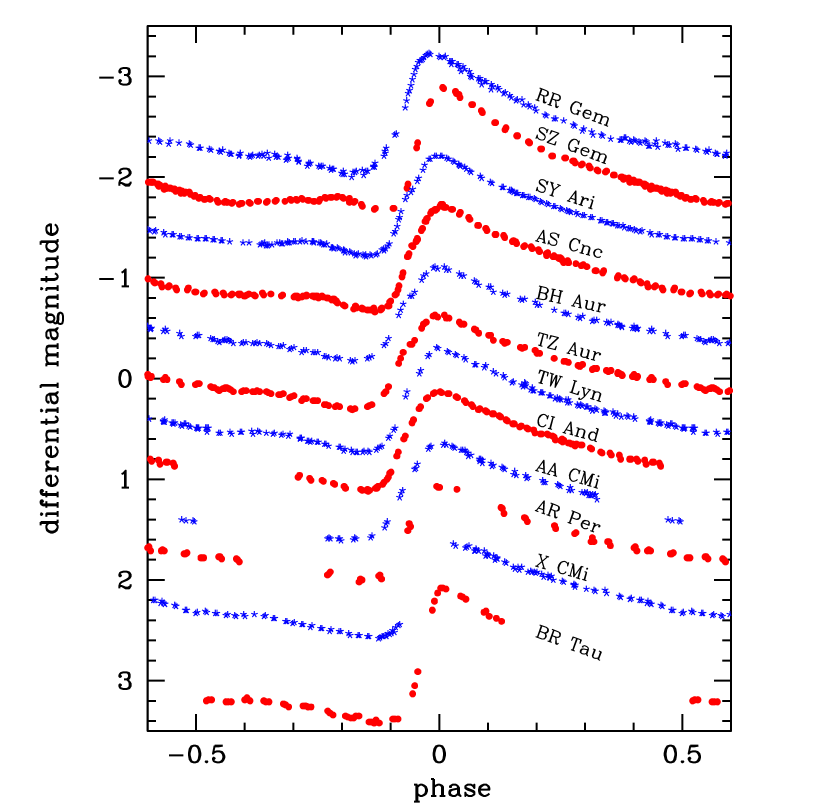
Figure 1: Lightcurves of the RR Lyrae stars in $y$. Data from subsequent cycles have been combined (see Table 1 for observing dates). The curves have been shifted arbitrarily in $y$ to fit them into one panel. For the stars lower in the figure, the lightcurve coverage is incomplete.

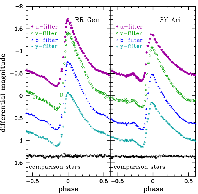
Figure 2: Lightcurves of RR Gem and SY Ari observed with Busca in the Strömgren-system. Note the different brightness amplitude of the two stars. At the bottom, the instrumental brightness of the mean of two comparison stars (selected in the field of each variable) is shown.

2 Observations and data reduction

The observations were carried out in three sessions at the Calar Alto Observatory of the Deutsch-Spanisches Astronomie Zentrum (DSAZ) in southern Spain in three successive winter seasons, between 4 and 9 Jan. 2005, between 16 and 19 Dec. 2005, and between 26 and 28 Nov. 2006.

The times of maximum brightness within the observing sessions were calculated for each star from the period $P$ and a reference epoch as $V_{\rm max}={\rm JD}({\rm ref.epoch}))\times(nP)$ with appropriate $n$. This allowed optimal phase-coverage planning of the photometry. In the various figures to follow, the data are plotted against phase $\Phi$ based on the observed maximum. For a few stars, the maximum could not be measured so the phase was determined from early epoch maxima.

Our programme consisted of observing 18 relatively bright RR Lyrae (for accurate positions and additional data, see Maintz 2005). Of 12 of these, (almost) complete lightcurves were obtained (coverage $>$70%) as given in Table 1 and Fig. 1 (and Fig. 2). However, for X CMi we missed the maximum. Of 6 stars (GM And, OV And, GI Gem, TY Cam, TT Lyn, CZ Lac), only smaller portions (15 to 57%) of the light curve could be obtained; these stars are not discussed further.

The stars selected are fundamental mode pulsators (see Fig. 3). They generally have lightcurve bumps.

Table 1: The stars with basic information, the J.D. of the observations, and the phase ranges covered

Star	CI And	SY Ari	AR Per	BR Tau	BH Aur	TZ Aur
RA	01 55 08.29	02 17 34.04	04 17 17.19	04 34 42.89	05 12 04.26	07 11 35.01
DEC	43 45 56.47	21 42 59.26	47 24 00.63	21 46 21.72	33 57 46.95	40 46 37.13
mean $y$ ;  $E(B-V)$  [mag]	11.86 ; 0.22	12.21 ; 0.25	9.40 ; 0.73	11.96 ; 0.31	11.43 ; 0.19	11.43 ; 0.19
distance [pc] ;  [M/H]	1741 ; $-$0.83	2100 ; $-1.4:$	612 ; $-$0.43	1835 ; $-0.7:$	1400 ; +0.14	1500 ; $-$0.79
period [d]	0.484728	0.5666815	0.425551	0.3905928	0.456089	0.39167479
exp. time [s] $v,b,y$; $u,b,y$	40; 40	70; 70	20; 60	70; 210	70; 210	30; 30
start of observations
at JD = 2453370.	+5.2914	+5.2947				+5.6153
phase covered	0.82 to 1.26	0.66 to 1.05				0.67 to 0.95
	+7.4215	+7.2612				+6.4747
	1.21 to 1.43	0.13 to 0.65				0.86 to 1.60
		+8.3353				+7.5535
		1.03 to 1.16				0.62 to 0.97
		+9.2568				+8.3106
		0.65 to 0.91				0.55 to .89
at JD = 2453720.	+1.32			+3.2969	+1.2980
phase covered	0.66 to 0.85			0.53 to 1.14	0.52 to 1.39
					+2.5868
					0.34 to 0.54
at JD = 2454060.			+7.2981	+7.5013
phase covered			0.75 to 1.63	0.73 to 0.87
Star	AA CMi	RR Gem	X CMi	TW Lyn	SZ Gem	AS Cnc
RA	07 17 19.17	07 21 33.53	07 21 44.62	07 45 06.29	07 53 43.45	08 25 42.11
DEC	01 43 40.06	30 52 59.45	02 21 26.30	43 06 41.56	19 16 23.93	25 43 08.80
mean $y$ ; $E(B-V)$ [mag]	11.13 ; 0.16	11.03 ; 0.22	12.23 ; 0.35	11.91 ; 0.16	11.45 ; 0.13	12.58 ; 0.16
distance [pc] ;  [M/H]	1220 ; $-$0.15	1260 ; $-$0.29	1766 ; $-$0.71	1549 ; $-$0.66	1601 ; $-$1.46	2324 ; $-$1.89
period [d]	0.476327	0.397292	0.57138	0.481862	0.5011270	0.61752
exp. time [s] $v,b,y$; $u,b,y$	40; 40 / 20; 60	20; 20	70; 70	40; 40	20; 20	40; 40
start of observations
at JD = 2453370.		+5.5257	+8.6759	+6.5937	+5.5385	+7.5695
phase covered		0.98 to 1.49	1.08 to 1.17	1.16 to 1.51	0.39 to 0.77	0.73 to 1.05
		+6.4776	+9.3641	+7.2652	+6.4800	+8.4688
		0.38 to 1.10	0.29 to 0.93	0.55 to 0.76	1.26 to 1.48	1.18 to 1.63
		+8.5121		+8.3421	+7.6349	+9.4268
		0.50 to 0.88		0.79 to 1.25	0.57 to 0.84	0.73 to 1.28
				+9.2625
				0.70 to 0.76
at JD = 2453720.	+2.4285		+1.5757		+1.5348	+1.4625
phase covered	0.77 to 1.09		1.21 to 1.32		0.82 to 1.28	0.59 to 0.69
at JD = 2454060.	+6.6066		+6.6110
phase covered	1.02 to 1.32		1.07 to 1.28

M/H] (in logarithmic units) estimated from our $m_{1}$ (see Sect. 3).

Busca (Reif et al. 1999) is operated at the 2.2m telescope of the Calar Alto Observatory. Busca splits the telescope beam above the Cassegrain focus via dichroic beam splitters in 4 wavelength channels between 3200 and 9000 Å, with edges at 4300, 5400 and 7300 Å. Each channel is equipped with a (4k)² CCD. In each channel, a filter wheel allows the placement of appropriate filters.

For the measurements we used the Strömgren $u,v,b,y$-system, extended by the Cousins $I$ band. The $y$ band is close to the cut-off of a Busca-dichroic filter; however, the transformation of $y$ into the standard system could be performed without problems. Because of the proximity of the wavelengths of $u$ and $v$, their filters are in the same Busca channel. Since the $u$ and $v$ bands could not be measured simultaneously, the photometry alternated between the simultaneous exposures in $y,b,v,(I)$ and $y,b,u,(I)$. For two stars, light curves in the four Strömgren-bands are shown in Fig. 2. More data are shown in Maintz (2008a).

Figure 3: Plot of the amplitude in $y$ versus period of our stars showing that they are fundamental mode RRa-type pulsators. The band between the dotted lines marks the zone of RRa and RRb pulsators (see Ledoux & Walraven 1958).

To calibrate the data, the instrumental brightness of each variable was obtained by comparison with two non-variable stars in the field. Where possible, one star with a brightness near the $y_{\rm max}$ of the RR Lyrae star was used and another of brightness close to $y_{\rm min}$ of the variable. (In the data a known suspected variable was quantified; see Maintz 2008b.) The airmass correction was obtained from these comparison stars.

To secure the absolute calibration, we observed appropriate stars from the list of Perry et al. (1987) at moments in the light cycle of the variable where the changes in brightness were small or monotonous. The instrumental magnitudes of the (airmass-corrected) photometry were related to the true magnitudes of the calibration stars. This permitted the calibration of the RR Lyrae star photometry. First, the RR Lyrae $y$ measurements were calibrated. Since the instrumental $(b-y)_{\rm inst}$ from Busca is more accurate than $b_{\rm cal}$-$y_{\rm cal}$ (the same is true for the other indices), the calibrated $b-y$ and $v-b$ were obtained from the instrumental index and that of the calibration stars. The sequentially obtained colour indices $u-y$ and $v-y$ were then used to interpolate in time to obtain $u-v$, which was calibrated. Using these indices, $c_{1}=(u-v)-(v-b)$ and $m_{1}=(v-b)-(b-y)$ were calculated.

The RR Lyrae star CCD photometry was performed with equal exposure times throughout the cycle, of 20 s for the brightest and 70 s for the faintest stars. Exposure times are given in Table 1. For three stars the exposure times in the $u,b,y$ measurements were $3\times$ those of the $v,b,y$ measurements (see Table 1). The (simultaneous) reading-out of the CCDs took about 2 min. Thus the CCD exposures followed each other quickly, within 2.5 min for the brighter stars and 3.5 min for the fainter ones. The short exposure times did not lead to large time smearing, not even when the star changed quickly in brightness. In most cases, two stars were observed alternatingly in rapid succession to achieve good light curve coverage for as many stars as possible. This alternation explains why most light curves presented have data intervals longer than 3.5 min.

Basic data ($d$, $E(B-V)$, [M/H]) were taken from Beers et al. (2000), Fernley et al. (1998), and Layden (1994), in part taking averages. Some of the stars are known to be behind gas with extinction and we corrected for that using expressions given by Clem et al. (2004). For four stars we calculated $d$ from $M_{V}$ based on [Fe/H] using the formula of Fernley et al. (1998). The adopted distances are given in Table 1.

3 Colour-index loops

For three stars the run through the cycle of the derived absolutely calibrated colour indices is shown in Fig. 4. The $b-y$ versus $c_{1}$ diagram for two typical stars from our sample, RR Gem and TZ Aur (Fig. 5, left panel), shows clear colour index loops. The index $m_{1}$ varies in line with $c_{1}$ (Fig.4). Figure 5 (right panel) shows the very moderate $m_{1}$ loops in a colour-colour plot.

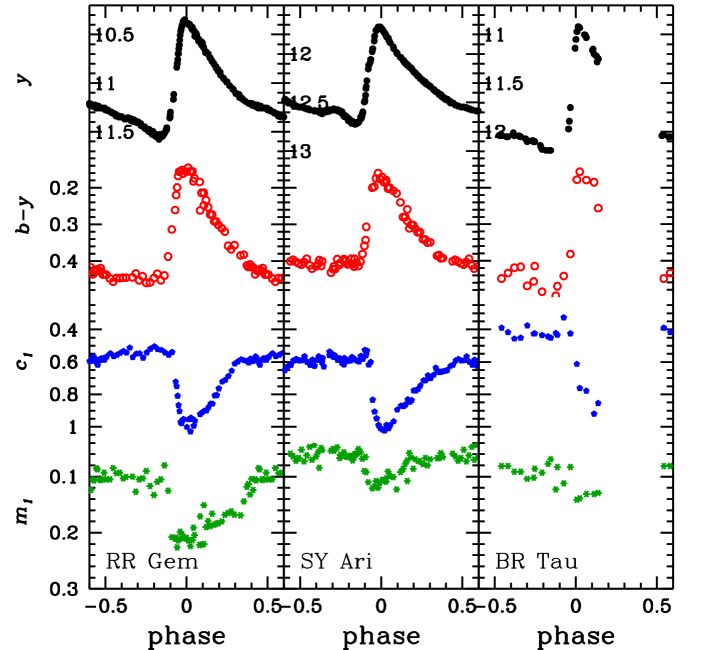
Figure 4: Lightcurves in the calibrated Strömgren-indices of the stars RR~Gem, SY Ari, and BR Tau. The phase coverage of the photometry can be reconstructed from the information given in Table 1 (for BR~Tau the coverage is only 70%) and can be recognised in Fig. 1.

The ($c_{1}$,$b-y$) curves show the interplay of the surface parameters $\log g$ and $T_{\rm eff}$ during the cycle. The loop is essentially due to $c_{1}$, which represents (above $T_{\rm eff}\simeq 6000$ K) the strength of the Balmer jump. At low $T_{\rm eff}$, the Balmer level is hardly populated. When the temperature increases (bluer $b-y$), $T_{\rm eff}$ and $n_{e}$ (and thus $\log g$) of the atmosphere gas increase and (collisional) excitation of hydrogen becomes noticeable. When the temperature decreases the population of the Balmer level decreases as well. In RR Lyrae star atmospheres, the ionisation of hydrogen hardly plays a role (except for an increase in $n_{e}$) because the highest temperatures in the pulsational cycle are $T_{\rm eff}<9000$ K.

It is evident from the data that the highest temperatures appear when the star is close to maximum light. During most of the period, the measured colour indices indicate low temperatures (large $b-y$, small $c_{1}$), as visible in the clump of data points in the lower-right corner of the left-side panels of Fig. 5. The brightening leg and the dimming leg of the colour curves do not overlap. During brightening, $b-y$ changes faster than $c_{1}$, which is indicative of a faster rise in $T_{\rm eff}$ than in the excitation to the Balmer level. In the dimming branch the converse is found (see Fig. 5, left). Thus the colour curve exhibits hysteresis.

As for the loops in $m_{1}$ (Fig. 5 right), these are quite moderate and do not show much in the sense of hysteresis. The change in $m_{1}$ over the cycle is on average 0.1 mag ($m_{1}$ is largest at maximum light). For our stars, $m_{1}$ is larger for stars known to have larger [M/H] (see also the calibration for red giant stars by Hilker 2000), while for stars with [M/H] $<-1$ dex $m_{1}$ is only marginally metal dependent. At the $T_{\rm eff}$ of RR Lyrae stars, cycle variations in $m_{1}$ related to the [M/H] are small. Nevertheless, using these trends, we estimated [M/H] for the two stars for which these values were unavailable from other sources (see Table 1). The variation in $m_{1}$ over the cycle must be caused by changes in temperature and electron density, which both influence the level of ionisation and excitation of ions.

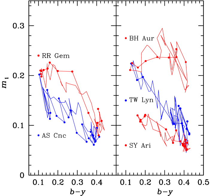
Figure 5: Colour loops in $b-y,c_{1}$ (at left) and in $b-y,m_{1}$ (at right) of several stars. The data points of the brightening phase are marked with $\bullet$.
Left: Clear hysteresis-like behaviour in $b-y,c_{1}$ is shown for RR Gem and TZ Aur. Arrows mark the direction of time. At phases between 0.3 and 0.85 (see Fig. 4), the colour index $c_{1}$ seems to just scatter. The $b-y,c_{1}$ combination represents mostly $T_{\rm eff}$ but also Balmer excitation.
Right: Colour loops in $b-y,m_{1}$ (shown for RR Gem, AS Cnc, SY Aur, TW Lyn, and SZ Gem) marginally exhibit hysteresis-like behaviour. The index $m_{1}$ generally represents metal content [M/H], its change in RR Lyrae stars is mostly due to changing $T_{\rm eff}$.

4 Behaviour of atmospheric parameters

4.1 Deriving parameters in the stationary case

The parameters $T_{\rm eff}$ and $\log g$ were determined from our photometry using the conversion grids given by Clem et al. (2004). These grids are based on modelled spectral energy distributions and are provided in steps of 0.5 dex of metal content [M/H]. Clem et al. made extensive calibrations of the Strömgren system against the parameters of non-variable stars. They show that individual Population II star colours can be matched with models to within $\simeq$200 K and $\simeq$0.1 dex, showing what is the ultimate uncertainty of a match. For Population I stars, the effect of small variations in metal content (0.3 dex) on the colours, and thus on the derived $T_{\rm eff}$ and $\log g$, is small. The dependence of colours on metal content is significant only for $T_{\rm eff}<6000$ K. For each star we used the grid for which [M/H] was closest to the metal content of each star.

The parameters $T_{\rm eff}$ and $\log g$ can be used to derive additional parameters describing the behaviour of the stellar atmosphere. The conditions in a regularly pulsating stars are in “quasi-hydrostatic equilibrium” (Cox 1980; Ch. 8.3), meaning that the use of a calibration based on stable stars is justified.

However, when a RR Lyrae star brightens from $V_{\rm min}$ to $V_{\rm max}$ within approximately one hour, the atmosphere is probably not in quasi-hydrostatic equilibrium. Doubling of Ca and H lines has been seen (e.g., Struve 1947, Sanford 1949) and H lines have been seen in emission (e.g., Preston & Paczynski 1964) in that part of the RR Lyrae cycle, which according to Abt (1959) originate from dynamic effects. Since no models exist that take these effects for photometry into account there is no other option than to use static models. Furthermore, the light we detect comes from the photosphere, i.e., the layer in which, at the particular wavelength observed, the optical depth is $\tau$ $\simeq$ $0.7$. This means that in the course of the pulsational cycle it is not necessarily the same gas from which the light detected emanates. We return to these aspects later (Sect. 8.2).

The luminosity of a star is related to the surface parameters $R$ and $T_{\rm eff}$ through the familiar equation $L=4\pi R^{2}\cdot\sigma T_{\rm eff}^{4}$, which can be rewritten in the relative logarithmic form

$$\log{\Bigl{(}\frac{L}{L_{\odot}}\Bigr{)}}=2\log{\Bigl{(}\frac{R}{R_{\odot}}\Bigr{)}}+4\log{\Bigl{(}\frac{T}{T_{\odot}}\Bigr{)}}\ \ \ .$$ (1)

The surface gravity of a star is defined as $g={\rm G}\ {M}/{R^{2}}$. This expression can be transformed into a logarithmic one relative to solar values given by

$$\log{\Bigl{(}\frac{g}{g_{\odot}}\Bigr{)}}=\log{\Bigl{(}\frac{M}{M_{\odot}}\Bigr{)}}-2\log{\Bigl{(}\frac{R}{R_{\odot}}\Bigr{)}}\ \ \ .$$

Using Eqs. 1 and 4.1, one can then eliminate the radius so that the combined equation has the stellar mass, temperature, gravity, and luminosity as variables,

$$\log{\Bigl{(}\frac{L}{L_{\odot}}\Bigr{)}}+\log g=4\log{T_{\rm eff}}+\log{\Bigl{(}\frac{M}{M_{\odot}}\Bigr{)}}-10.68\ \ \ ,$$ (2)

where $-10.68=(\log T_{\rm eff}-\log g)_{\odot}$ in cgs units. This equation can be used to calculate $\log g$.

4.2 Deriving parameters in the pulsating case

In a pulsating atmosphere the parameters $T_{\rm eff}$, $\log g$, and $R$ vary continuously (note that no time subscripts are used in this paper).

$\bullet$ $T_{\rm eff}$, $L$.   The time-dependent values $L$ and $T_{\rm eff}$ can be derived from the photometry if one knows the stars distance. $T_{\rm eff}$ is simply inferred from a calibrated $b-y$ (using the grid of Clem et al. 2004). $L$ has to be determined from $y$, the integral over the spectral energy distribution and the distance $d$ of the star.

As for $L$, an RR Lyrae star has the convenient property that the maximum of its spectral energy distribution (in $B_{\lambda}$) lies close to the middle of the visual wavelength band, near Johnson $V$ or Strömgren $y$. This is true during the entire cycle: $T_{\rm eff}$ actually varies only between roughly 5000 and 9000 K. This means that the bolometric correction is neither large nor varies a lot. We have performed the bolometric correction using the classic values of Schmidt-Kaler (1982). We fitted a quadratic equation in the temperature range relevant for RR Lyrae stars.

Distances were adopted as described in Sect. 2. If the distance $d$ of a star were off by 20%, this would result in an error of 0.08 in $\log L$.

Results for $L$ and $T_{\rm eff}$ are shown in Fig. 6.

$\bullet$ $R$.   The radius can be calculated from Eq. 1. For examples of radius change see Fig. 7.

$\bullet$ $\log g$, $\log g_{\rm BJ}$, $\log g_{\rm eff}$.   The surface gravity $g$ can be calculated from Eq. 2 if one knows the luminosity of the star (discussed above) and its mass (see below). This gravity is like an overall equilibrium gravity and is henceforth called $g(T,L,M)$.

There is a further aspect affecting the gravity. In a pulsating atmosphere, the actual surface gravity ($g(T,L,M)$ at the level $\tau\simeq 0.7$) is modified due to acceleration of the atmosphere during the pulsation cycle with respect to the “normal” gravity. Thus, $g$ is modified by an acceleration term, $d^{2}R/dt^{2}$. The total gravity is called the “effective” gravity

$$g_{\rm eff}=g(T,L,M)+\frac{d^{2}R}{dt^{2}}\ \ \ ,$$ (3)

indicating the vertical gravitational force in the atmosphere.

The time-dependent Strömgren photometry measures the actual condition of a stellar atmosphere. The gravity derived from $b-y,c_{1}$ is a function of gas density, visible in the excitation of the Balmer level and in $c_{1}$ representing the Balmer jump. We will call this gravity the “Balmer-jump” gravity, $\log g_{\rm BJ}$. This gravity is independent of $\log g_{\rm eff}$ and instead represents the pressure of the gas sampled, i.e., $P_{\rm gas}=f(T,\rho)$.

We will return to the values derived for $\log g(T,L,M)$ and $\log g_{\rm BJ}$ in Sect. 9.

$\bullet$ $M_{V}$, $M$.   RR Lyrae star distances have thus far been derived using a reference value for $M_{V}$. This value of $M_{V}$ does not apply to all RR Lyrae stars since horizontal-branch (HB) stars evolve over more than $\Delta\log L=0.1$ on the HB. If, e.g., $M_{V}$ of a star were to differ by 0.25 mag from the reference value adopted, $L$ would be off by 0.10.

The mass of RR Lyrae stars is in the range from $0.6$ to $0.8$ M_⊙. We adopted a mass of $M=0.7$ M_⊙, thereby considering that our RR Lyrae stars can deviate 15% from that value. This deviation propagates to a maximum deviation of 0.06 dex in a calculated $\log g(T,L,M)$.

A few observational determinations of the absolute magnitude $M_{V}$ and mass $M$ of horizontal-branch and RR Lyrae stars exist, such as those of de Boer et al. (1995), Moehler et al. (1995), de Boer et al. (1997), Moehler et al. (1997), Tsujimoto et al. (1998), and Gratton (1998).

We return to the effect of incorrect values of these reference parameters in Sect. 4.5.

The run of $T_{\rm eff}$, $\log g_{\rm BJ}$, and $R$ derived as described above are shown for three of our stars in Fig. 7. The shape of these curves is very similar to those presented by van Albada & de Boer (1975). But the data of Fig. 7 is less noisy because the photometry with CCDs is faster and more precise than possible with the slower photomultipliers of that time, and because of the simultaneity of the Busca measurements.

Table 2: Cycle averages of several RR Lyr star parameters

Star	$\langle L\rangle$	$\langle T_{\rm eff}\rangle$	$\log\langle g(T,L,M)\rangle$	$\log\langle g_{\rm BJ}\rangle$
RR Gem	43.5	6647	2.84	3.33
TW Lyn	31.6	6196	2.85	3.61
AS Cnc	49.3	6592	2.77	3.46
SY Ari	50.0	6059	2.61	2.93
SZ Gem	52.9	6739	2.78	3.38
BH Aur	46.4	5997	2.63	3.04
TZ Aur	50.3	5934	2.58	2.86
AR Per	56.3	6030	2.55	3.66
CI And	47.7	6270	2.69	3.19
BR Tau	44.	5980	2.65	2.92
AA Cmi	45.	6340	2.73	3.28

4.3 Phase resampling in steps of 0.02

To facilitate the calculation of averages over the phase and additional analyses, we resampled the curves of $L$, $T_{\rm eff}$, $R$, and $\log g_{\rm BJ}$ as derived from the observational data using steps of $\Delta\Phi=0.02$ (starting with $i=0$ near maximum light). These resampled values (given henceforth with subscript 0.02) can be easily integrated (fixed time step). The result of these resamplings can be seen as curves in Figs. 6 and 7 (and in further figures).

Time averages over the cycle of our stars have been calculated based on the 0.02 phase stepped lightcurves. For a few stars, the lightcurve coverage was not complete and we made reasonable interpolations in the gaps to obtain the time averages.

4.4 Time-averaged quantities

The structure of a “non-pulsating RR Lyr star” is given by the time-averaged parameters $\langle T_{\rm eff}\rangle$, $\langle L\rangle$ and $\langle g\rangle$. The time-averaged gravity, $\langle g\rangle$, has in a purely periodic system zero contribution from $d^{2}R/dt^{2}$.

Oke and collaborators and van Albada & de Boer felt that since $g$ varies strongly, the “average” value is best derived from the quiet part of the cycle, i.e., from $0.3<\Phi<0.85$. However, Fig. 9 makes clear that this has shortcomings. In that phase interval, $\log g(T,L,M)$ is (for most stars) lower than average by between 0.1 and 0.2 dex, because the atmosphere is then slowly but continuously contracting (but see Sect. 9).

The time-averaged quantities of essential parameters were calculated from the resampled curves in steps of $\Delta\Phi=0.02$ (see above), the integral was derived as the sum of 50 values. Thus

$$\langle T_{\rm eff}\rangle=\int T_{\rm eff}\ dt=\bigl{(}\Sigma_{i=1}^{50}\ (\,(T_{\rm eff})_{0.02})\,_{i}\bigr{)}\ /\ 50$$ (4)

and

$$\langle L\rangle=\bigl{(}\Sigma_{i=1}^{50}\ (L_{0.02})\,_{i}\bigr{)}\ /\ 50\ \ \ ,$$ (5)

individual values of $L_{0.02}$ being calculated as described in Sect. 4.2. The averages of the two gravity versions are

$$\langle g(T,L,M)\rangle=\bigl{(}\Sigma_{i=1}^{50}\ (\,g(T,L,M)_{0.02})\,_{i}\bigr{)}\ /\ 50$$ (6)

and

$$\langle g_{\rm BJ}\rangle=\bigl{(}\Sigma_{i=1}^{50}\ (\,(g_{\rm BJ})_{0.02})\,_{i}\bigr{)}\ /\ 50\ \ \ .$$ (7)

Time-averaged values for 11 stars are given in Table 2 and are for four stars included in Fig. 6. It can immediately be seen that the values of $\langle g(T,L,M)\rangle$ and $\langle g_{\rm BJ}\rangle$ are quite dissimilar. We discuss this further in Sect. 9.

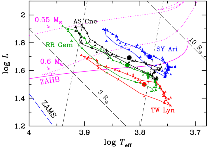
Figure 6: For four RR Lyrae (TW Lyn, RR Gem, AS Cnc, and SY Ari), the run of $T_{\rm eff}$ and $L$ is shown in an HRD. The originally derived values are plotted as 3-pointed stars, the resampled curve (in steps of 0.02 in phase, Sect. 4.3) is shown as a full line. The mean values over the cycle (from Table 2) are given as $\bullet$. The background data (ZAMS, metal-poor ZAHB, the evolution tracks of a 0.55 and a 0.6 M_⊙ HB star) are taken from de Boer & Seggewiss (2008; Fig 10.9). Two lines of constant $R$ are indicated. The almost vertical dashed lines mark the approximate location of the pulsational instability strip from Gautschi & Saio (1995). The stellar surface parameters of the RR Lyrae show hysteresis.

4.5 Error budget

In our analyses, the following uncertainties had to be taken into account.

Photometric errors are, given the instrumental characteristics of Busca, small. We estimated the uncertainties in $y$ to be 0.03 mag. The bolometric corrections are small and introduce errors of up to 2%. This leads to a total typical photometric uncertainty in $L$ of 3%. In the colour indices $b-y$, $m_{1}$, and $c_{1}$, the uncertainties are 0.02 mag (smaller than the error in $y$ because of the simultaneity of the measurements).

We used distances from the literature. The effect of their uncertainties on $L$ is given below.

To obtain $T_{\rm eff}$ and $\log g_{\rm BJ}$, the indices $b-y$ and $c_{1}$ were used with the grid of Clem et al. (2004). The grid is not perfect and reading $T_{\rm eff}$ and $\log g_{\rm BJ}$ from that grid by eye, we assessed that (based on readings performed three times for the entire cycle for one star) the uncertainty in $T_{\rm eff}$ is about 1%, and in $\log g_{\rm BJ}$ about 0.05 dex. Since the effects of metallicity, [M/H], are only significant for $T_{\rm eff}<6000$ K, which occurs for only 3 of our less well-observed stars near minimum light, we are confident that our error estimates are only at those temperatures affected by a possibly small mismatch in [M/H].

Given the measurement uncertainties in $L$ (3%) and $T_{\rm eff}$ (1%), it follows that the uncertainty in the calculated $R$ values is 4%. If, in addition, a distance were incorrect by +10% that would give an additional offset for a given star in $R$ of +5%.

As mentioned in Sect. 4.2, we assumed a fixed mass for all stars of 0.7 M_⊙, and indicated a margin of error of 15%. This error would lead for a given star to an offset of 0.06 dex in a calculated $\log g(T,L,M)$.

The values of $\log g(T,L,M)$ calculated from Eq. 2 have a measurement error of about 8% or 0.03 dex. A distance error of +10% leads to an offset in $\log g(T,L,M)$ of $-$0.04, an error in the mass $M$ of +10% to an offset in $\log g(T,L,M)$ of +0.04.

Finally we note that the distances of RR Lyrae have essentially all been derived from a reference $M_{V}$ (distance from distance modulus), in some cases adjusted for metal content, [Fe/H]. For a review of the latest calibrations we refer to Sandage & Tamman (2006). However, in spite of all calibration efforts, $M_{V}$ has a spread in $M_{V}$ of between 0.2 and 0.4 mag for a given [Fe/H] or an uncertainty of even up to 1.0 mag if [Fe/H] is unknown. Moreover, given the evolution of RR Lyrae stars on the HB, a single and universal value of $M_{V}$ does not exist anyway; the evolution of an HB star may lead to an increase in $\log L$ of 0.5 dex when reaching the terminal-age HB (see, e.g., de Boer & Seggewiss 2008; their figure 10.9). Therefore, if a considered star were brighter than the chosen reference value, its derived distance modulus and thus distance would be too small. If the true $M_{V}$ of the star is unbeknown to be 0.25 mag brighter than the reference value, the distance (as given in Table 1) will turn out to be too small by 12%. This affects the derived $L$, then being too small by 0.10 dex.

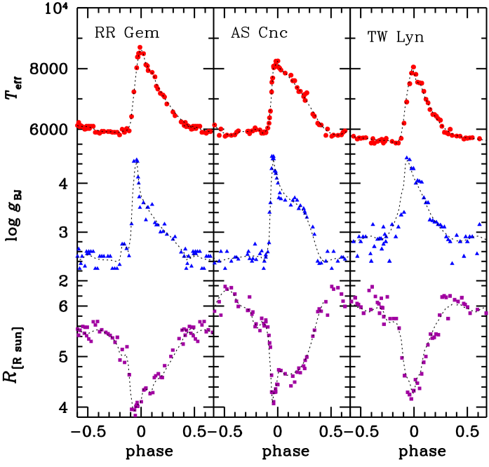
Figure 7: Run of the parameters $T_{\rm eff}$, $\log g_{\rm BJ}$, and $R$ (derived as described in Sect. 4.2) during the pulsational cycle of RR Gem, AS Cnc, and TW~Lyn using the calibration grid by Clem et al. (2004). The thin dashed lines are the values resampled at $\Delta\Phi$ = 0.02 (see Sect. 4.3).

The mean values of Table 2 were derived from a large number of individual measurements, so the observational scatter is basically cancelled. What remains is the error related to the calibration grid and also the error in the assumed distance and/or $M_{V}$ (affecting $\log g_{\rm BJ}$ and $L$ as just indicated, as well as $R$).

5 Hysteresis of the parameters $T_{\rm eff}$, $R$, and $\log g_{\rm BJ}$

The values of the atmospheric parameters for all points in the cycle were derived from the photometry as described above. In Fig. 6 we show the run of $T_{\rm eff}$ and $L$ of four of our stars in an HRD. These parameters exhibit loops through the diagram extending over and beyond the instability strip. The loopings are reminiscent of hysteresis. In the older literature, the lagging behind in the change of some parameter compared to another parameter is called “phase-lag” (see, e.g., Cox 1980).

The behaviour of $T_{\rm eff}$ and $\log g_{\rm BJ}$ against phase (Fig. 7) shows remarkable features. For all stars, $\log g_{\rm BJ}$ begins to increase about $\Delta\Phi=0.05$ before $T_{\rm eff}$ starts to increase. Furthermore, $\log g_{\rm BJ}$ reaches its highest value when $T_{\rm eff}$ has increased about halfway to its maximum value. And when $T_{\rm eff}$ reaches its maximum, $\log g_{\rm BJ}$ is already decreasing (at phase $\simeq 0$). The resulting value of $R$ (that of Fig. 7 is derived from Eq. 1) indicates that $R$ is smallest when $\log g_{\rm BJ}$ is largest.

The run of $R$ shows that RR Lyrae are relatively extended stars for about half of the cycle ($0.25<\Phi<0.75$), while large changes in radius take place between $0.75<\Phi<1.25$, with the most rapid change occurring between $0.9<\Phi<1.15$. At $\Phi\simeq 0.9$, a drastic reduction in the derived $R$ takes place (the atmosphere apparently starts to collapse), reaching the smallest $R$ near $\Phi\simeq 0.95$. At smallest $R$ the atmosphere must have a high density. Up to the highest density, $T_{\rm eff}$ is at the same level as in the quiet phase leading up to the collapse. Soon after $\Phi\simeq 0.95$, $R$ increases again.

In general, when $y$ is brightest $T_{\rm eff}$ is at its highest and $R$ is very small; but immediately after minimum light, at the high peak in $\log g_{\rm BJ}$, $R$ is at its smallest.

6 Spectral line strengths

For three of our stars (TZ Aur, RR Gem, RS Boo), spectra were obtained (in January 2006, independently of the Strömgren-photometry) with the focal reducer spectrograph at the 1 m telescope of the Observatory “Hoher List” of the AIfA. Radial velocities could not be obtained with this instrument. The spectra have a resolution of $\sim$3 Å. Because of telescope size and focal-reducer set-up, exposure times had to be rather long, of the order of 3% of the period, leading to phase smearing. We determined the equivalent withs of the lines of H$\alpha$, H$\beta$, H$\gamma$, Na i D, and Ca ii K.

For RR Gem and TZ Aur, we show (Fig. 8) how the strengths of the H$\gamma$ and Ca K lines vary during the cycle. Results for RS Boo are not shown because the lightcurve coverage was poor.

H$\gamma$. The strength of Balmer lines is governed by $T_{\rm eff}$ as expected since the Balmer level can be populated only during the higher $T_{\rm eff}$ part of the RR Lyrae cycle. The temporal behaviour of $W$(H$\gamma$) and $T_{\rm eff}$ (Fig. 8) is indeed very similar.

Ca ii K. The strength of Ca K is predominantly set by the gas density, i.e., the ionization balance forces Ca ii to be reduced at higher density (when $R$ is smallest). The curves of $W$(CaK) and $R$ are very similar in terms of their temporal behaviour (clearly for RR Gem).

The Na i D absorption is very weak and provides little information, except that Na i D is strong when $T_{\rm eff}$ is at its lowest; the increased strength is caused by the shift of the ionization balance towards the neutral state at lower $T_{\rm eff}$.

7 The variation in the pulsation velocity $V_{\rm pul}$

7.1 The coarse variation in $V_{\rm pul}$

Figure 7 shows for three stars the change in radius, $R$, as derived from Eq. 1. One can thus calculate the velocity of the stellar atmosphere (the “pulsation velocity”, $V_{\rm pul}$). We used

$$V_{\rm pul}=\frac{\Delta R}{\Delta t}=\frac{R_{\Phi}-R_{\Phi+\Delta\Phi}}{t_{\Phi}-t_{\Phi+\Delta\Phi}}\ \ \ ,$$ (8)

where $R$ is at intervals of fixed value $\Delta\Phi=0.02$ (see Sect. 4.4). To avoid being affected by peaks in the noise we applied a running triangular (1,2,1) smoothing to the curves of $R$ before calculating $V_{\rm pul}$. In Fig. 9, $V_{\rm pul}$ (as well as the smoothed $R$) is given for eight stars with the best data. Note that $V_{\rm pul}$ plotted is that seen from the centre of the star (and is not a heliocentric value).

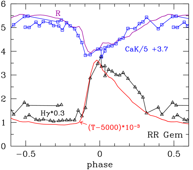
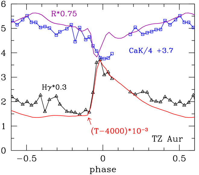
Figure 8: For RR Gem and TZ Aur, the run of the equivalent widths $W$ of the spectral lines Ca ii K and H$\gamma$ are shown and compared with the parameters $R$ and $T_{\rm eff}$ (as in Fig. 7). The vertical scale is that of $R$ [R_⊙] of RR Gem. The values of the other parameters ($W$ in Å and $T_{\rm eff}$ in K) have been renormalized to fit this vertical scale (see the labels to the curves). For RR Gem, H$\gamma$ is proportional to $T_{\rm eff}$ and is strongest when $T_{\rm eff}$ is largest (stronger excitation); Ca K is weakest when the radius $R$ is smallest (at constant $T$ and higher density, $n_{e}$ shifts the ionization balance). The spectral observations of RR Gem come from two nights in the same time frame as but independent of the Strömgren photometry (explaining the overlap of data in phase). In TZ Aur the relation of $R$ with Ca K is less clear. The spectra of TZ Aur did not cover the entire light curve (gap near $\Phi=0.15$).

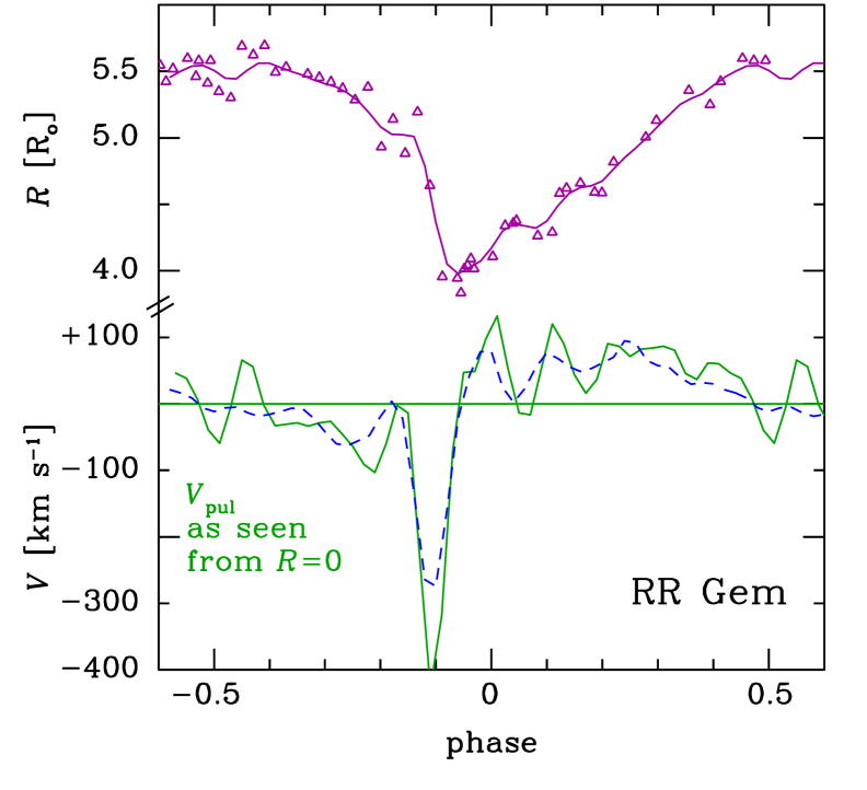
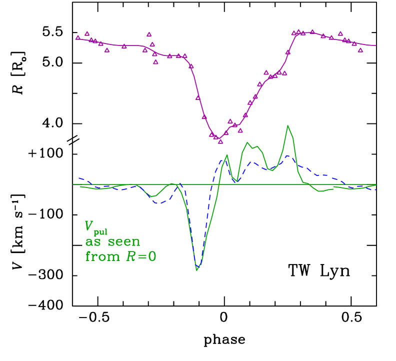
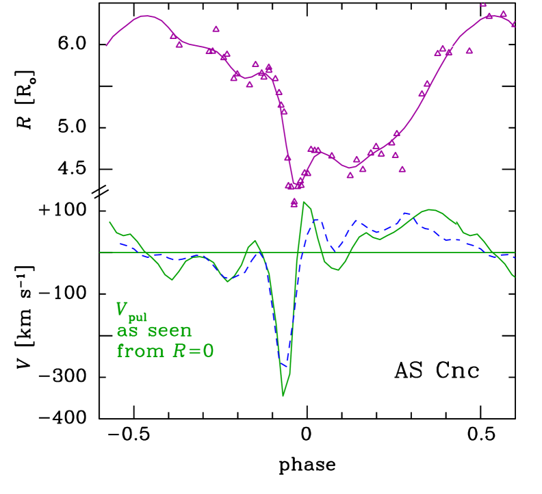
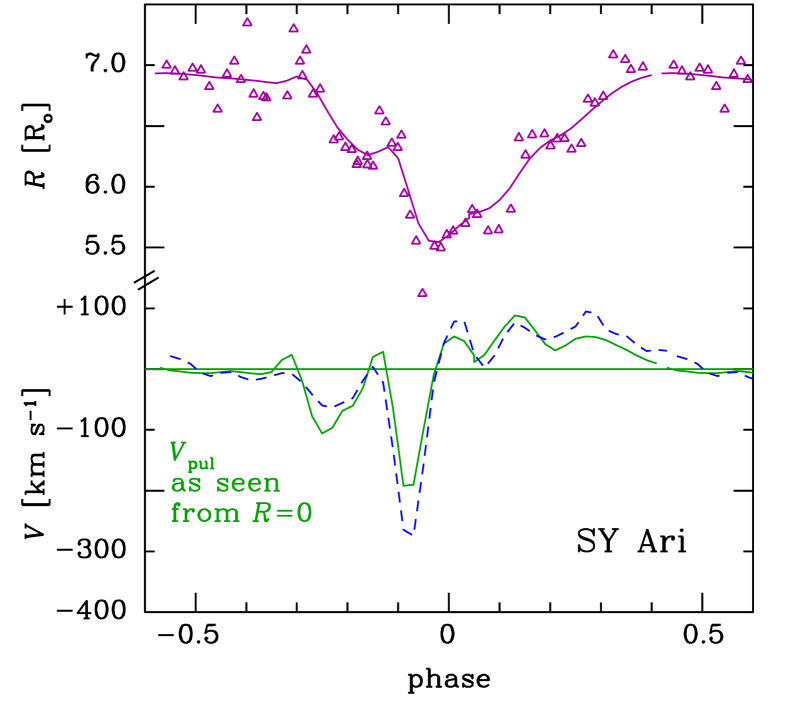
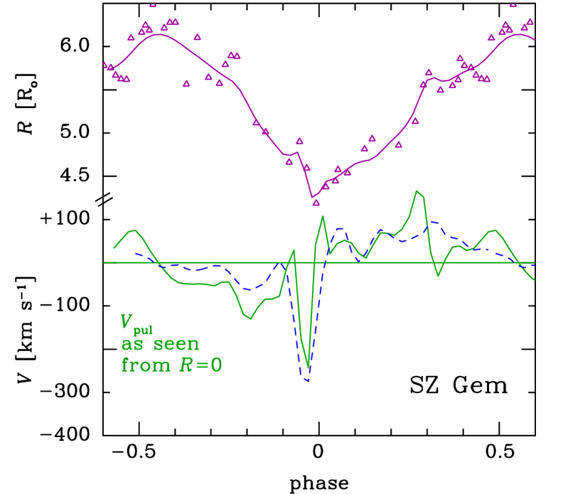
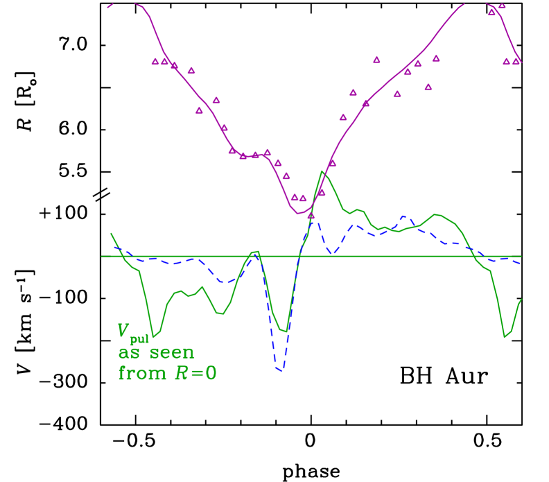
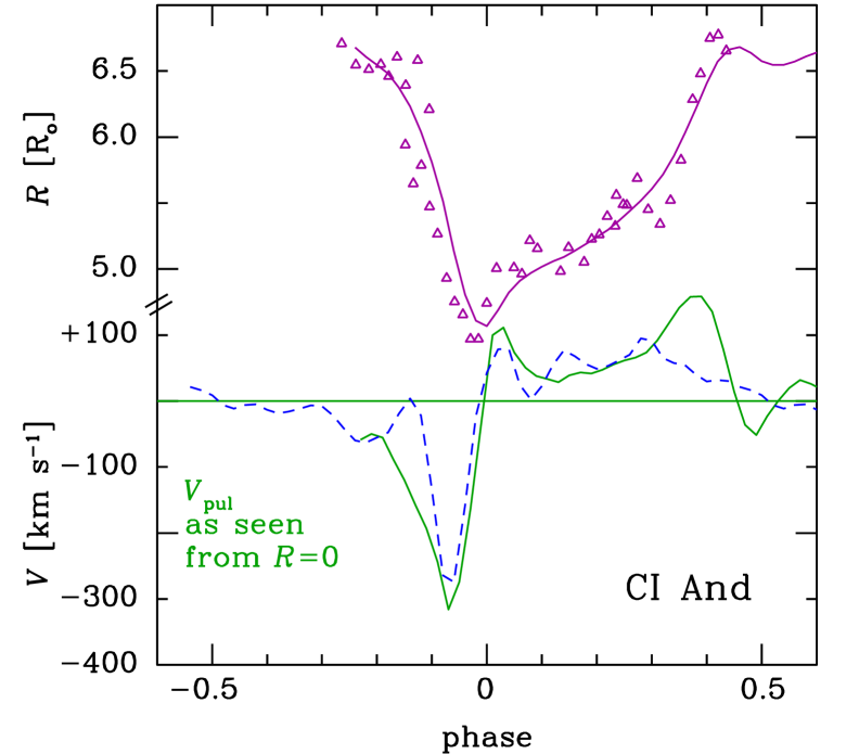
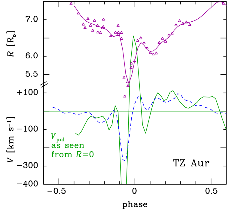
Figure 9: The change in $V_{\rm pul}$ is shown together with the change in $R$ (note that the scale of $R$ differs from panel to panel). Top row: the “well behaved” and well-observed stars. Bottom row: the stars with less well behaved $V_{\rm pul}$-curves (partly due to poor light-curve coverage and to interpolation). Top curve and data in each panel: The values of $R$ were calculated from photometric data using Eqs. 1 and 4.1 (as in Fig. 7). The resampled data ($\Delta\Phi=0.02$) were used to derive the variation in $R$ over these intervals. The curves shown give the resampled values after an additional running triangular (1,2,1) smoothing. Note that, for several stars, the period was not fully covered by our observations. Bottom curves in each panel: The run of $V_{\rm pul}$ as derived from the smoothed $R$-curve is shown. To guide the eye, a line at $V_{\rm pul}$=0 km s^-1 is added. The average of the $V_{\rm pul}$ curves of the four well observed stars (the stars shown in the top row) has also here been added as a dashed line (for each star a small appropriate phase shift was added). Clearly, the wiggles in $V_{\rm pul}$ are not noise but are systematic $V_{\rm pul}$-variations. This is confirmed by the stars of the bottom row, whose $V_{\rm pul}$ curves were not included in the calculated average. The average $V_{\rm pul}$ curve shows a rhythm with a period of about $P/7$.

The calculated variation in $V_{\rm pul}$ over the cycle (see Fig. 7) has a general pattern. There is a pronounced minimum close to $\Phi\simeq 0.95$ where $V_{\rm pul}\simeq-150$ to $-400$ km s^-1, followed by a steep rise to a level of $V_{\rm pul}\simeq+50$ to 100 km s^-1. In the course of the cycle, $V_{\rm pul}$ then slowly decreases and slowly becomes negative reaching a level of $V_{\rm pul}\simeq-50$ km s^-1. A sudden additional decrease sets then in to reach the most negative value of $V_{\rm pul}$, the value this description started with. It shows that the atmosphere really collapses between $\Phi=0.9$ and $1.0$. Thereafter, the expansion is drastic but beyond $\Phi\simeq 0.05$ it is far more gradual (at $V_{\rm pul}\simeq 50$ km s^-1) as it decelerates.

The behaviour of $V_{\rm pul}$ is similar to that of a model atmosphere as presented in the gedankenexperiment by Renzini et al. (1992). That gedankenexperiment had a star with a core and an envelope, in which the luminosity offered to the base of the envelope, $L_{\rm B}$, was manipulated. A gentle decrease in this $L_{\rm B}$ from a high $L_{\rm B}$ state could be accommodated by the envelope until some critical value of $L_{\rm B}$ at which the envelope collapsed. Then, in the gedankenexperiment, $L_{\rm B}$ was raised again and the now compact atmosphere slowly expanded until some other critical value of $L_{\rm B}$ was reached, now leading to a run-away expansion.

In the case of RR Lyrae, the run of $L$ is controlled by the opacity in the He⁺-He⁺⁺ ionization boundary layer. With increasing transmission of energy through the envelope, $L$ increases and the star expands until at some limit the envelope has become so tenuous that (since $L$ can no longer increase) it must collapse.

Having determined the run of $V_{\rm pul}$ one can derive $\frac{d^{2}R}{dt^{2}}$. These acceleration values change considerably during the pulsational cycle. However, because of the uncertainty in all $V_{\rm pul}$ values due to opacity effects to be discussed in Sect. 8, we refrain from commenting on these acceleration values.

7.2 The detailed variation in $V_{\rm pul}$ and a correlation with $P$

The small-scale variations in the curves of $V_{\rm pul}$ (Fig. 9) might be regarded as due to photometric noise. However, on closer inspection there is significant structure.

We selected the well-behaved $V_{\rm pul}$-curves to determine an average $V_{\rm pul}$-curve for an RR Lyr star. For that, we chose the stars RR Gem, TW Lyn, AS Cnc, and SY Ari (the top row panels in Fig. 9). Before the curves can be added for averaging, small phase shifts were applied because the chosen $y_{\rm max}$ was not perfectly aligned with the epoch relation and the resampling at 0.02 intervals in phase may also have introduced small phase shifts. Figure 9 shows the results for these stars. It is evident that the wiggles in the $V_{\rm pul}$-curves are very similar for these four stars. For the four less well-observed stars not included in the averaging, a comparison with the average $V_{\rm pul}$-curve shows that these stars have also the same behaviour in $V_{\rm pul}$.

For all stars, the wiggles in the average $V_{\rm pul}$ indicate that after the collapse the envelope oscillates (continues to oscillate) with a rhythm of about 1/7 of the period $P$. This rhythm at $P/7$ is the same for all our stars, independent of their actual period. It is as if the envelope has a residual oscillation triggered by the collapse. The collapse itself occurs from $V_{\rm pul}$$\simeq 0$ through the highest collapse velocity back to $V_{\rm pul}$$\simeq 0$ km s^-1, which is a time equal to about $P/7$.

One might suspect that $P/7$ is due to our resampling at 0.02 phase intervals, the period being (almost) exactly 7 of our data points. However, we note that Paparó et al. (2009) reported a specific role of the 7th harmonic in one well-studied CoRoT RR Lyr star. The CoRoT data do not have the 0.02 phase resampling rhythm. Barcza (2003) found in the RR Lyr star SU Dra from photometry an “undulation”’ of $P/5$. It is unclear what the cause of these periodicities is.

8 Comparison with literature data and optical depth effects

We derived the time-dependent radius of each star from our photometry and from its change the velocity of the atmosphere. The analysis above was performed without considering analyses of other RR Lyrae data presented in the literature.

A well-known method for deriving the radius of RR Lyrae stars is the Baade-Wesselink method, where the radial velocities observed over the cycle are integrated to infer the variation in radius (see, e.g., Liu & Janes 1990). This method has been applied to several RR Lyrae stars.

8.1 Comparison with other results

For two of our stars (RR Gem and AR Per), cycle velocities were presented by Liu & Janes (1989). Their velocities were obtained by cross-correlating their RR Lyrae star spectra with spectra of two standard stars, one of spectral type F6 IV and one of A2 IV. The values they derived from the two standard stars are very similar so, that their final velocity curves are based on just the standard of type A2 IV.

Our velocity curve for RR Gem has a shape quite different from the one of Liu & Janes (1989). Note that in their figure 5 they give the observed radial velocity, whereas in our Fig. 9 the velocity as seen from the stellar centre is given. Their velocity curve shows a large speed away from the stellar centre at $\Phi\simeq 0$ followed by a gradual slowing down to approach the minimum in velocity at $\Phi\simeq 0.7$. The velocity curves of other RR Lyrae stars of Liu & Janes show the same behaviour. The amplitude in their velocity curves is $\simeq$60 km s^-1. Adopting the usual geometry factor $p=1.32$ (see Liu & Janes 1990; but see Fernley 1994) to convert from observed radial velocity to pulsational velocity, their velocities translate into an amplitude in $V_{\rm pul}$ of $\simeq$80 km s^-1.

On the other hand, our stars have amongst themselves similar behaviour. Their outer layers experience during the cycle only a modest change in velocity except for a rapid fall toward the stellar centre as of $\Phi\simeq 0.85$ to a fastest centre approach at $\Phi\simeq 0.95$, followed by a rapid decline in velocity to reach a modest expansion velocity near $\Phi\simeq 0.05$. In our data, the full amplitude of the velocity $V_{\rm pul}$ is $\simeq$300 km s^-1.

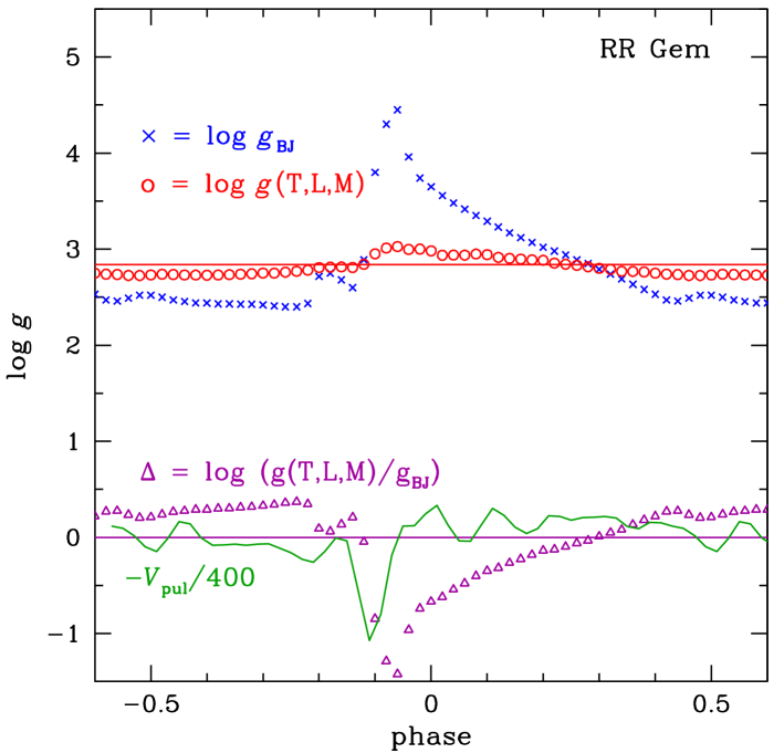
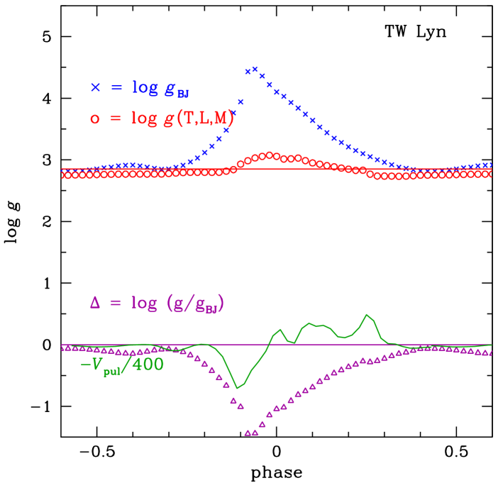
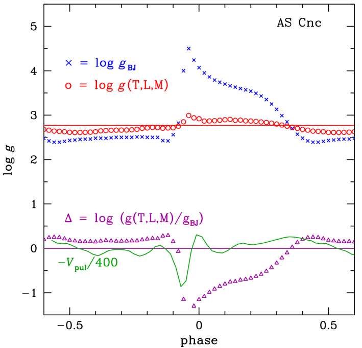
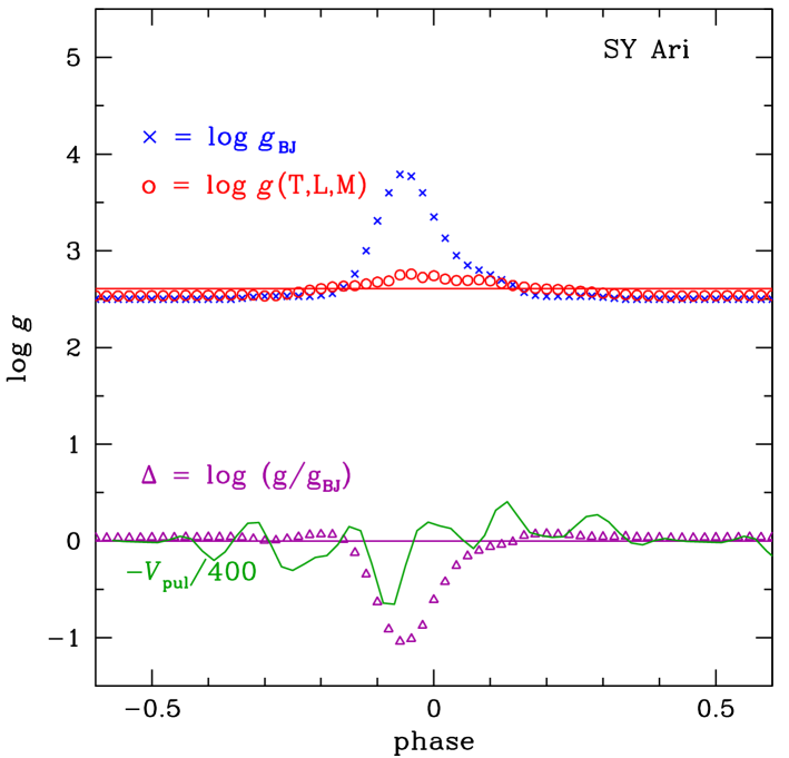
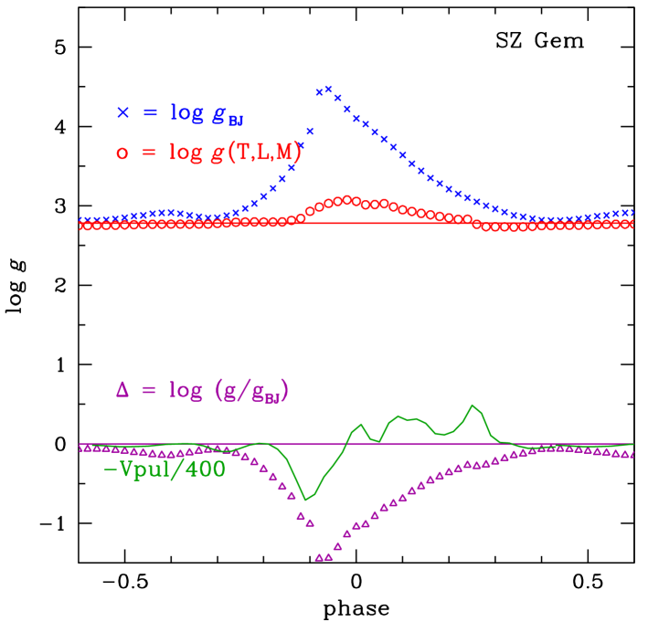
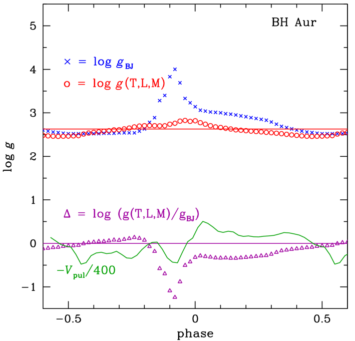
Figure 10: Run of the two aspects of $\log g$ (resampled data, see Sect. 4.3) for the well observed stars. Top curves: The slowly varying curve is $\log g(T,L,M)$ derived from Eqs. 1 and 4.1 (thus using $T$ and $L$ derived from $y$,$b-y$), and the full horizontal line gives the average of $\langle g(T,L,M)\rangle$ over the cycle (in logarithmic form; see Table 2). The peaked curve shows the gravity, $\log g_{\rm BJ}$, derived from the $b-y,c_{1}$ photometry and the grid calibrated to obtain $T_{\rm eff}$ and $\log g_{\rm BJ}$. Bottom curves: the ratio $g(T,L,M)/g_{\rm BJ}$ is shown on a logarithmic scale. Clearly, when $\Delta=\log(g(T,L,M)/g_{\rm BJ})<0$ the atmosphere gas must be quite compressed. The curve of $V_{\rm pul}$ has added (in units as in Fig. 9).

The difference between our velocity curves and those of Liu & Janes is mostly caused by the drastic reduction of $R$ we find at $\Phi\simeq 0.9$. Eliminating this behaviour from our $R$ curves (eliminating the $R$ data for $0.85<\Phi<0.05$) results in a velocity amplitude of $V_{\rm pul}$ of up to $\simeq$90 km s^-1, quite similar to the one of Liu & Janes mentioned above. In short, the radius change of an RR Lyrae star based on the Baade-Wesselink radial velocity curves does not chime with the pronounced change in $R$ we derived (using Eq. 1) from the photometry. This difference is almost certainly caused by effects of optical depth.

8.2 Effects of optical depth $\tau$

When analysing our data we tacitly assumed that the detected light originates, throughout the cycle, in the same gas and thus from the same atmospheric layer. Such assumptions have been made in almost all analyses of variable star data (also with the Baade-Wesselink method), but they need not be correct. Furthermore, Abt (1959) noted that the continuum light originates in layers with $\tau\simeq 0.7$ while the spectral lines rather are formed in layers with $\tau\simeq 0.3$.

During the cycle, compaction of the atmosphere and/or changes in level of ionization may lead to changes in $\tau$ in that gas, thus to different layers being sampled in the photometry. This is also the case for spectral lines: changes in the density and temperature of a layer due to vertical motion will lead to changes in the local ionization balance and the excitation state of ions, thus to a varying strength of the relevant absorption lines. During the cycle a spectral line may therefore form in different gas layers. Furthermore, the strength of a line formed at greater depths is also influenced by the level of photon scattering filling in the spectral line.

The phase lag between lines from metals and hydrogen discovered by van Hoof & Struve (1953) in a $\beta$ Cepheid star has been attributed to similar optical depth effects. For RR Lyrae stars, this “van Hoof effect” was studied by, e.g., Mathias et al. (1995) and Chadid & Gillet (1998). Our sketchy spectral data (Fig. 8, Ca ii and H$\gamma$) exhibit a phase lag too, which can easily be attributed to changes in the gas conditions that also cause the hysteresis in $T_{\rm eff}$ and $\log g_{\rm BJ}$.

In spectra of several RR Lyrae stars, line doubling has been reported near $\Phi=0$ (see, e.g., Sanford 1949). Considerable increases in line width may also occur near that phase (e.g., Fe ii lines; see, e.g., Chadid 2000). Spectral line doubling implies that there are gas layers in the same line of sight with the same ions but which are at different (radial) velocities. This doubling is seen mostly in the lower level Balmer series lines but also in other intrinsically strong lines such as Ca H&K. Thus, the spectral absorption in those lines comes from different geometric depths in the atmosphere. Note that when for the determination of radial velocities template spectra are used, any velocity differences between ionic species are averaged out.

8.3 Photometry and spectroscopy sample different layers

Consider an outward moving dense layer of the stellar atmosphere. Upon its expansion and cooling, its continuum optical depth becomes smaller. Thus, the level of $\tau\simeq 0.7$ from which the continuum light emerges moves physically downward through the gas, leading to smaller photometrically derived $R$ values. If this intrinsic $\tau$-level moves rapidly, the concomittant rapid decrease in derived $R$ is naturally interpreted as an extremely rapid downward velocity, even when the gas itself hardly has a vertical motion. The level from which the (metal) spectral lines emerge (near $\tau\simeq 0.3$) will exhibit this effect later, i.e., only after the gas has been lifted further to larger radii (cooled and rarefied further to lower $\tau$). This happens later than the change in the gas levels releasing the continuum light. In this case, geometrically deeper levels may then be (spectroscopically) sampled suggesting a decrease in $R$ even if the gas itself still moves outward. We note one can see a difference in that sense between lines of Fe ii and Fe i (Chadid & Gillet 1998). Finally, the intrinsically strong lines, such as the lower Balmer series lines and a few other lines with large intrinsic absorption capability, will exhibit this effect yet later. However, in deeper layers (at different radial velocity) the local Balmer absorption may already show up with its own radial velocity ($\lambda$-shifted with respect to the Balmer line in higher layers), thus leading to line-doubling from lower levels of the Balmer series.

The presented data do not allow us to asses the details of these optical depth effects. We emphasize that the parameters derived from the photometry always refer to the conditions in the layer with $\tau\simeq 0.7$, the layer from which the measured continuum light emanates. It may be that some of our interpretations need to be revised once more detailed measurements of the particular gas layers would be available.

The differences between our run of $R$ (and of $V_{\rm pul}$ derived from it) and the Baade-Wesselink run of $V_{\rm rad}$ (and of $R$ derived from it) can be understood as being caused by the sampling of layers with different $\tau$. The Baade-Wesselink method samples layers with $\tau$ smaller than $\tau$ of the layers sampled with continuum photometry. It thus is unsurprising that the run of $R$ as derived from these methods differs in important ways, all due to the physical condition ($\tau$) of the gas layer from which the measured radiation (be it spectral lines or the continuum) emerges.

At the end of Sect. 7.2 it was noted that oscillations are visible in $V_{\rm pul}$ with $P/7$. Perhaps these variations are also caused by temporal small optical depth effects ($T_{\rm eff}$ and $\log g_{\rm BJ}$) and do not represent fluctuations in gas velocity.

9 The variations in $\log g(T,L,M)$ and $\log g_{\rm BJ}$, and verifications of distance and mass

The run of $\log g(T,L,M)$ was derived from Eq. 2. The actual surface gravities, $\log g_{\rm BJ}$, were derived from $b-y,c_{1}$. In Fig. 10 we plot three parameters: $\log g(T,L,M)$, $\log g_{\rm BJ}$ and the logarithmic ratio $\log(g(T,L,M)/g_{\rm BJ})$. When $\log g(T,L,M)-\log g_{\rm BJ}<0$ (or $\log(g(T,L,M)/g_{\rm BJ})<1$) the atmosphere is clearly compressed (collapsed).

The data in Fig. 10 indicate that in the quiet part of the cycle ($0.4<\Phi<0.8$) the gravity $\log g(T,L,M)$ is, for several stars, not equal to $\log g_{\rm BJ}$. However, in those quiet parts of the cycle, all parameters are apparently stable (there are most likely no optical depth effects at this point) and so we would expect $\log g(T,L,M)$ and $\log g_{\rm BJ}$ to be equal there. We can explore how one might adjust $d$ and $M$ to make $\log g(T,L,M)$ from Eq. 2 equal to $\log g_{\rm BJ}$ in that phase interval. For RR Lyrae stars, that phase ($\Phi\simeq 0.6$) has $T_{\rm eff}\simeq 6000$ K, only a little higher than $(T_{\rm eff})_{\odot}$.

The distances of our stars were defined as described in Sect. 2. They are taken from the literature and they are primarily determined from an adopted reference value of $M_{V}$. For some stars we calculated $d$ from $M_{V}$ (including effects of [Fe/H]).

We recall from Sect. 4.5 (on the error budget) that the sum of the measurement errors in $\log g(T,L,M)$ and $\log g_{\rm BJ}$ may be as large as 0.08 dex. If these two gravities were to be equal and if we assumed the full margin of error of 0.08, then, e.g., $\log g(T,L,M)$ for RR Gem should be reduced by $\simeq$0.22 dex, that of AS Cnc by $\simeq$0.12, while that of TW Lyn should be larger by $\simeq$0.07 dex.

If the adopted $M_{V}$ (or $d$) and $M$ of our stars were wrong and had to be changed, this would produce (when using Eq. 2) the tabulated effects:

assumed change			effects
$M_{V}$	($d$)	$M$	$\log g(T,L,M)$	$L$	$R$
$-0.20$	$+10$%		$-0.04$	$+20$%	+10%
		+10%	+0.04	-	-

We note again that changing the distance is for the stars observed only implicit; distances of RR Lyrae stars have (except for those in the papers referred to in Sect. 4.2) not been determined by other means than through $M_{V}$. Thus only $M_{V}$ or the mass $M$ can be changed.

For our stars a change in either $M_{V}$ or $M$ (or perhaps a combination thereof) is needed to make $\log g(T,L,M)$ and $\log g_{\rm BJ}$ match. The changes in $M_{V}$ indicated below are within the range permissible by the non-uniqueness of $M_{V}$, as mentioned in Sect. 4.5. For the stars shown in Fig. 10 the changes are:
- RR Gem: $M_{V}$ 1.0 mag brighter, $M$ 50% smaller. The optimum would be to change $M_{V}$ leading to $L$ larger by a factor 2.5 (0.4 dex in $\log L$). Reducing the mass by 50% is no option, it then would be too low. A combination of changes might also fit.
- TW Lyn: $M_{V}$ 0.4 mag fainter, $M$ 20% larger. Changing $M_{V}$ is not the right option because its $L$ value would, in Fig. 6, be even further below the ZAHB. Hence $M$ should be 20% higher at 0.85 M_⊙. Note that (in Fig. 6) the mean value of $L$ can be made larger when adopting a yet larger mass.
- AS Cnc: $M_{V}$ 0.6 mag brighter, $M$ 30% lower. Changes similar to but smaller than those for RR Gem would be needed.
- SY Ari: no changes are needed within the errors.
- SZ Gem: $M$ smaller by 0.1 dex, to give $M=0.56$ M_⊙.
- BH Aur: no changes are needed within the errors.
- TZ Aur: to make the two gravities match, $\log g(T,L,M)$ should be $\simeq$0.3 dex lower. This would be achieved if $M$ were considerably lower. Alternatively, $M_{V}$ should (with $M=0.7$ M_⊙) be so much brighter, that $L$ is doubled. In both cases, TZ Aur would then be a well-evolved HB star.

We do not comment on the less well-observed stars (the bottom four in Table 2).

10 The lightcurve bump

The stars in our programme were primarily selected from the class said to have lightcurve “bumps”. These bumps in the run of brightness need not be very pronounced (for $y$-magnitudes see Fig. 1). One goal of the observations was to investigate whether these bumps in brightness affect the colours of the stars. Examples of the bump region for a few stars are given in Fig. 11.

First, we note that most of our stars with good light-curve coverage hardly show the light-curve bump in the Strömgren colour indices. Among these are TW Lyn, BH Aur, X CMi, TZ Aur, BR Tau, and RR Gem, which have either a prolonged low level bump or no clear colour-index bump at all. While SY Ari has a bump in $y$ that has no effect in its colour indices, AS Cnc does show an effect. For the other stars, light-curve coverage was either poor or missing in this range of phases.

In AS Cnc the brightening and dimming is clearly recognisable and takes place in a short timespan. We note that the colour indices $u-b$ and $u-v$ change before $y$ brightens. Both indices become bluer meaning that the Balmer continuum radiation brightens without an increase in $T_{\rm eff}$. In this part of the cycle, the atmosphere is cool and the Balmer continuum brightening could mean that the gas cools even further leading to an additional reduction in opacity based on the lower Balmer level excitation. Since $T$ has not yet changed, the changes should be due to a reduction in gas density. Does extra light escape because of the lower $\tau$? At this point in the cycle, the atmosphere is quite extended and about to shrink. This happens at $\Phi\simeq-0.1$ (see Fig. 11 and earlier ones).

Bono & Stellingwerf (1994) attribute the bump feature to shockfronts.

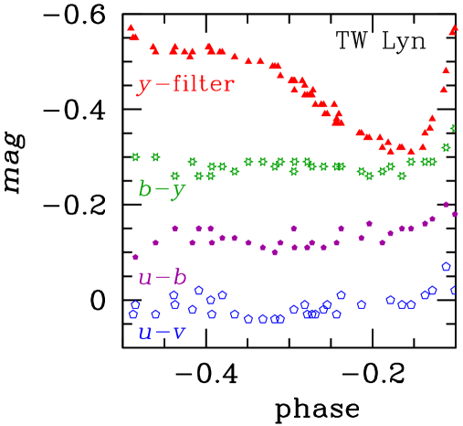
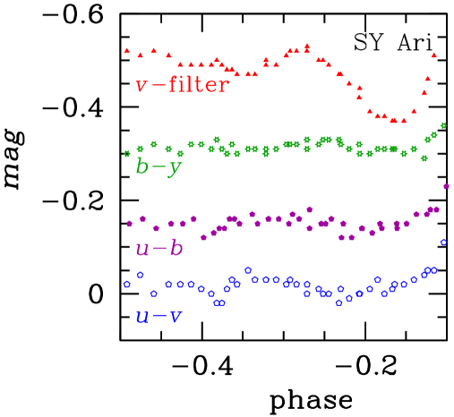
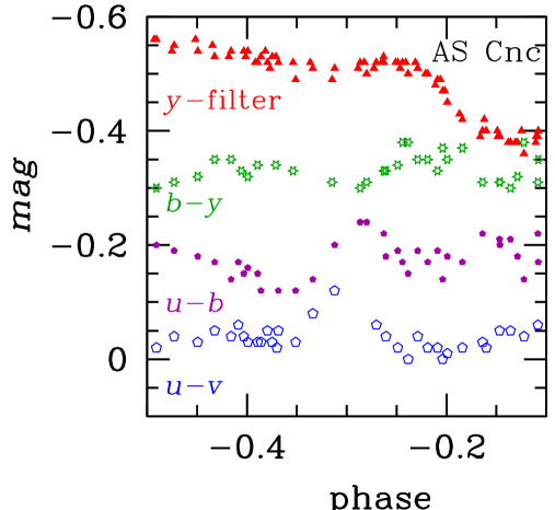
Figure 11: Three examples of Strömgren-photometry light curves of RR Lyrae stars near the possible “bump” in brightness. TW Lyn either does not show a bump or its bump is rather extended in phase; there is no or little effect on the colour indices. SY Ari does exhibit a bump in $y$ but there are no effects in its colour indices. For AS Cnc, the colour indices $u-b$ and $u-v$ clearly change before $y$ changes, indicating a change in the Balmer jump before a brightness change. The index $b-y$ (representing temperature) changes somewhat later.

11 Further remarks

11.1 Comparison with models

Numerous models have been constructed for the pulsation and for various other detailed aspects of RR Lyrae (see, e.g., Fokin et al. 1999). A comparison with models is of limited value since most models are one-dimensional. More importantly, it is not always clear how theory has been transformed to observables. Do the theoretical predictions for $V$, $R$, spectral line strengths, and velocities all refer to information from the layer with the relevant $\tau$ (thus to what one really would observe) or to a matter-defined gas layer?

Parameters of RR Lyrae stars have been determined using different kinds of data and with different modelling. We refer to the analysis of Sódor et al. (2009) for results based on the Baade-Wesselink method and its refinements as well as to additional literature.

11.2 Blazhko effect

A good portion of RR Lyrae stars shows cycle-to-cycle variations in their light curves, the so-called Blazhko effect (for references see, e.g., Jurcsik et al. 2009). Some of the stars of our sample are also known to be Blazhko stars but they exhibit these variations only at a moderate level. However, these variations may affect the stellar parameters derived. The data we acquired cover to short a time span to address and assess possible cycle-to-cycle variations in the stellar parameters.

11.3 Relation between stellar mass and kinematics

Six of our stars were part of the study of kinematics of RR Lyrae stars (Maintz & de Boer 2005). Of these, five (CI And, AR Per, TZ Aur, RR Gem, and TW Lyn) are stars of the disk population (according to their kinematics), while SZ Gem is a star with halo kinematics. Halo RR Lyrae are understood to be older than disk RR Lyrae, so should (on average) have a lower mass.

For TW Lyn, we found that its mass should be higher than the adopted reference value and instead be $\simeq$0.85 M_⊙, which chimes with it being a star of the disc. We note that Sódor et al. (2009) found a mass of $\simeq$0.82 M_⊙ for RR Gem, our analysis indicated $\simeq$0.7 M_⊙. For SZ Gem, we found a mass of $\simeq$0.56 M_⊙, this low mass being in line with the expected (larger age and) lower mass of halo stars.

BH Aur and SY Ari are found to correspond to the reference value of $M=0.7$ M_⊙, which is in line with their being disk stars.

12 Conclusions

Based on simultaneous Strömgren photometry and a comparison of the photometric indices with a calibrated $T_{\rm eff}$, $\log g$ grid, accurate atmospheric parameters of RR Lyrae stars have been determined. Curves of phase related runs of $\log g_{\rm BJ}$ (the gravity from the Balmer jump) and $T_{\rm eff}$ were derived. One can then calculate the change in radius of the stars over the cycle. By including additionally obtained spectra, one arrives at the following description of the behaviour of RR Lyrae stars.

The straightforward interpretation of the data derived for $R$ is that at phase $\Phi\simeq 0.9$ the atmosphere begins to collapse soon reaching a high gas density (when the star has its greatest brightness). This manifests itself in a large Balmer jump (large $\log g_{\rm BJ}$). Within an interval $\Delta\Phi\simeq 0.1$ the atmosphere then expands again.

An alternative interpretation is that at phase $\Phi\simeq 0.9$ the optical depth of the extended outer layers has become so small that the level of $\tau\simeq 0.7$ sampled in the photometry rushes through the gas inward mimicking a drastic reduction in radius. The contraction taking place anyway then elevates the density in that level having $\tau\simeq 0.7$, raising the optical depth there so that photometry subsequently samples layers again higher up in the atmosphere, suggesting a rapid expansion. The sudden increase in density manifests itself in lage values of $\log g_{\rm BJ}$.

During all these changes the atmosphere exhibits oscillation ripples with a rhythm of $P/7$.

A possible mismatch of the observed $\log g_{\rm BJ}$ and the calculated $\log g(T,L,M)$ in the quiet, descending part of the light curve can be used to assess the applicability of the mean parameters adopted for the stars, i.e., the absolute brightness $M_{V}$ (no geometric distances are known) and the mass $M$. One can then determine the individual values of $M_{V}$ and $M$ for a star.

Extending this kind of simultaneous Strömgren-photometry while avoiding multiplexing two stars would provide a much denser coverage of the light curves and thus a more accurate determination of the cycle variation in $R$. If spectra were then taken simultaneously, in which a range of spectral lines is included (lower and higher ionisation stages, strong and weak lines of the Balmer series) and of a nature to allow velocity determinations, one may hope to distinghuish the effects caused by the sampling of light from layers at different optical depth.

- (1) Abt, H. 1959, ApJ, 130, 824
- (2) Baade, W. 1926, AN, 228, 359
- (3) Barcza, S. 2003, A&A, 403, 683
- (4) Beers, T. C., Chiba, M., Joshii, Y., et al. 2000, AJ, 119, 2688
- (5) Bono, G., & Stellingwerf, R. F. 1994, ApJS, 93, 233
- (6) Breger, M. 1974, ApJ, 192, 75
- (7) Chadid, M. 2000, A&A, 359, 991
- (8) Chadid, M., & Gillet, D. 1998, A&A, 335, 255
- (9) Clem, J. L., VandenBerg, D. A., Grundahl, F., & Bell, R. A. 2004, AJ, 127, 1227
- (10) Cox, J. P. 1980, “Theory of Stellar Pulsation”, Princeton Univ. Press
- (11) Danziger, I. J., & Oke, J. B. 1967, ApJ, 147, 151
- (12) de Boer, K. S., Schmidt, J. H. K., & Heber, U. 1995, A&A, 303, 95
- (13) de Boer, K. S., & Seggewiss, W. 2008, “Stars and Stellar Evolution”; EDP Sciences
- (14) de Boer, K. S., Tucholke, H.-J., & Schmidt, J. H. K. 1997, A&A, 317, L23
- (15) Fernley, J. 1994, A&A, 284, L16
- (16) Fernley, J., Barnes, T. G., Skillen, I., Hawley, S. L., Hanley, C. J., Evans, D. W., Solano, E., & Garrido, R. 1998, A&A, 330, 515
- (17) Fokin, A. B., Gillet, D., & Chadid, M. 1999, A&A, 344, 930
- (18) Gautschy, A., & Saio, H. 1995, ARAA, 33, 75
- (19) Gratton, R. F. 1998, MNRAS, 296, 739
- (20) Hilker, M. 2000, A&A, 355, 994
- (21) Jurcsik, J., Sódor, Á., Szeidl, B., et al. 2009, MNRAS, 400, 1006
- (22) Layden, A. C. 1994, AJ, 108, 1016
- (23) Ledoux, P., & Walraven, Th. 1958, in Handbook of Physics, Vol LI, p.353
- (24) Liu, T., & Janes, K. A. 1989, ApJS, 69, 593
- (25) Liu, T., & Janes, K. A. 1990, ApJ, 354, 273
- (26) Lub, J. 1977a, PhD Thesis, Univ. Leiden
- (27) Lub, J. 1977b, A&AS, 29, 345
- (28) Lub, J. 1979, AJ, 84, 383
- (29) Maintz, G. 2005, A&A, 442, 381
- (30) Maintz, G. 2008a, PhD Thesis, Univ. Bonn
- (31) Maintz, G. 2008b, BAVSR, 57, 150
- (32) Maintz, G., & de Boer, K. S. 2005, A&A, 442, 229
- (33) Mathias, P., Gillet, D., Fokin, A. B., & Chadid, M. 1995, A&A, 298, 843
- (34) McNamara, D. H., & Feltz, K. A. 1977, PASP, 89, 699
- (35) Moehler, S., Heber, U., & de Boer, K. S. 1995, A&A, 294, 65
- (36) Moehler, S., Heber, U., & Rupprecht, G. 1997, A&A, 319, 109
- (37) Oke, J. B. 1966, ApJ, 145, 468
- (38) Oke, J. B., & Bonsack, S. J. 1960, ApJ, 132, 417
- (39) Oke, J. B., Giver, L. P., & Searle, L. 1962, ApJ, 136, 393
- (40) Paparó, M., Szabó, R., Benkó, J. M., et al. 2009, in “Stellar Pulsation: Challenges for Theory and Observation”, J.A.Guzik and P. Bradley (eds.), AIP Conf. Proc. 1170, p. 240
- (41) Perry, C. L., Olsen, E. H., & Crawford, D. L. 1987, PASP, 99, 1184
- (42) Preston, G. W., & Paczynski, B. 1964, ApJ, 140, 181
- (43) Reif, K., Bagschik, K., de Boer, K. S., Schmoll, J., Müller, Ph., Poschmann, H., Klink, G., Kohley, R., Heber, U., & Mebold, U. 1999, SPIE Vol. 3649, 109
- (44) Renzini, A., Greggio, L., Ritossa, C., & Ferrario, L. 1992, ApJ, 400, 280
- (45) Sandage, A., & Tamman, G. A. 2006, ARAA, 44, 93
- (46) Sandford, R. F. 1949, ApJ, 109, 208
- (47) Schmidt-Kaler, T. 1982, Landolt Börnstein; Mathematics for Engineers; X. Physics and Applied Physics for Engineers; Astronomy/Astrophysics
- (48) Siegel, M. J. 1982, PASP, 94, 122
- (49) Sódor, Á., Jurcsik, J., & Szeidl, B. 2009, MNRAS, 394, 261
- (50) Struve, O. 1947, PASP, 59, 192
- (51) Tsujimoto, T., Miyamoto, M., & Yoshi, Y. 1998, ApJ, 492, L79
- (52) van Albada, T. S., & de Boer, K. S. 1975, A&A, 39, 83
- (53) van Hoof, A., & Struve, O. 1953, PASP, 384, 158
- (54) Wesselink, A. J. 1946, Bull. Astr. Inst. Neth., 10, 83