Stability (over time) of Modified-CS and LS-CS for Recursive Causal Sparse Reconstruction

Abstract

In this work, we obtain sufficient conditions for the “stability” of our recently proposed algorithms, modified-CS (for noisy measurements) and Least Squares CS-residual (LS-CS), designed for recursive reconstruction of sparse signal sequences from noisy measurements. By “stability” we mean that the number of misses from the current support estimate and the number of extras in it remain bounded by a time-invariant value at all times. The concept is meaningful only if the bound is small compared to the current signal support size. A direct corollary is that the reconstruction errors are also bounded by a time-invariant and small value.

I Introduction

In this work, we study the “stability” of modified-CS (noisy) [1, 2] and of LS-CS-residual (LS-CS) [3, 4, 5] which were designed for recursive reconstruction of sparse signal sequences from noisy measurements. By “stability” we mean that the number of misses from the current support estimate and the number of extras in it remain bounded by a time-invariant value at all times. The concept is meaningful only if the bound is small compared to the current signal support size. A direct corollary is that the reconstruction errors are also bounded by a time-invariant and small value.

The key assumption that our algorithms utilize is that the support changes slowly over time. As we demonstrated in [3, 1], this assumption holds for many medical image sequences. Denote the support estimate from the previous time by $T$. Modified-CS tries to finds a signal that is sparsest outside of $T$ and satisfies the data constraint. LS-CS uses a different approach. It replaces compressive sensing (CS) on the observation by CS on the least squares (LS) residual computed using $T$. Both algorithms are able to achieve greatly reduced reconstruction error compared to simple CS (CS at each time separately) when using fewer measurements than what CS needs.

Other algorithms for recursive reconstruction include our older work on Kalman filtered CS-residual (KF-CS) [4, 5]; CS for time-varying signals [6] (assumes a time-invariant support, which is a somewhat restrictive assumption); homotopy methods [7] (use past reconstructions to speed up current optimization but not to improve reconstruction error with fewer measurements); and [8] (a recent modification of KF-CS). Two other algorithms that are also designed for static CS with partial knowledge of support include [9] and [10]. The work of [9] proposed an approach similar to modified-CS but did not analyze it and also did not show real experiments either. The work of [10], which appeared in parallel with modified-CS, assumed a probabilistic prior on the support and obtained conditions for exact reconstruction.

To the best of our knowledge, stability of recursive sparse reconstruction algorithms has not been studied in any other work except in our older works [3, 5] for LS-CS and KF-CS respectively. The KF-CS result [5] is under fairly strong assumptions, e.g. it is for a random walk signal change model with only support additions (no removals). The result for LS-CS stability [3] holds under mild assumptions and is for a fairly realistic signal change model. The only limitation is that it assumes that support changes occur “every-so-often”: every $d$ time units, there are $S_{a}$ support additions and $S_{a}$ removals. But from testing the slow support change assumption for real data (medical image sequences), it has been observed that support changes usually occur at every time, e.g. see Fig. 1 of [3]. This important case is the focus of the current work.

In [3], we only studied LS-CS (modified-CS was proposed later). But the techniques of [3] can be also used to show modified-CS stability for the model of [3]. In this work, we show the stability of both LS-CS and modified-CS and of its improved version, “modified-CS with add-LS-del”. We first discuss modified-CS since, from experiments, it is known to be a better algorithm. In facts its stability result is also better (holds under weaker assumptions).

The paper is organized as follows. We give problem definition in Sec. I-A and we overview our results in Sec. I-B. We describe the signal model for proving stability in Sec. II. We obtain sufficient conditions for the stability of modified-CS and discuss the implications in Sec. III. We discuss some of its limitations and develop a simple modification that uses a better support estimation approach (modified-CS with add-LS-del). This support estimation approach is related to the one in [11, 4, 3]. In Sec. IV, we show the stability of modified-CS with add-LS-del, which is more difficult to do. The result for LS-CS stability is obtained in Sec. V. Numerical experiments are discussed in Sec. VI. Conclusions are given in Sec. VII.

I-A Notation and Problem Definition

The set operations $\cup$, $\cap$, $\setminus$ have their usual meanings. $\emptyset$ denotes the empty set. We use $T^{c}$ to denote the complement of a set $T$ w.r.t. $[1,m]:=[1,2,\dots m]$, i.e. $T^{c}:=[1,m]\setminus T$. $|T|$ denotes the cardinality of $T$. For a vector, $v$, and a set, $T$, $v_{T}$ denotes the $|T|$ length sub-vector containing the elements of $v$ corresponding to the indices in the set $T$. $\|v\|_{k}$ denotes the $\ell_{k}$ norm of a vector $v$. If just $\|v\|$ is used, it refers to $\|v\|_{2}$. Similarly, for a matrix $M$, $\|M\|_{k}$ denotes its induced $k$-norm, while just $\|M\|$ refers to $\|M\|_{2}$. $M^{\prime}$ denotes the transpose of $M$ and $M^{\dagger}$ denotes the Moore-Penrose pseudo-inverse of $M$ (when $M$ is tall, $M^{\dagger}:=(M^{\prime}M)^{-1}M^{\prime}$). For a fat matrix $A$, $A_{T}$ denotes the sub-matrix obtained by extracting the columns of $A$ corresponding to the indices in $T$. The $S$-restricted isometry constant [12], $\delta_{S}$, for an $n\times m$ matrix (with $n<m$), $A$, and the $S,S^{\prime}$ restricted orthogonality constant [12], $\theta_{S,S^{\prime}}$, are as defined in [12, eq 1.3] and [12, eq 1.5] respectively.

We assume the following observation model:

$$y_{t}=Ax_{t}+w_{t},\ \|w_{t}\|\leq\epsilon$$ (1)

where $x_{t}$ is an $m$ length sparse vector with support $N_{t}$, $y_{t}$ is the $n<m$ length observation vector at time $t$ and $w_{t}$ is observation noise with $\|w_{t}\|\leq\epsilon$. “Support” refers to the set of indices of the nonzero elements of $x_{t}$.

Our goal is to recursively estimate $x_{t}$ using $y_{1},\dots y_{t}$. By recursively, we mean, use only $y_{t}$ and the estimate from $t-1$, $\hat{x}_{t-1}$, to compute the estimate at $t$.

As we explain in Sec. III, our algorithm need more measurements at the initial time, $t=0$. We use $n_{0}$ to denote the number of measurements used at $t=0$ and we use $A_{0}$ to denote the corresponding $n_{0}\times m$ measurement matrix. We use $\alpha$ to denote the support estimation threshold used by modified-CS and we use $\alpha_{add},\alpha_{del}$ to denote the support addition and deletion thresholds used by modified-CS with add-LS-del and by LS-CS.

We use $\hat{x}_{t}$ to denote the final estimate of $x_{t}$ at time $t$ and ${\hat{N}}_{t}$ to denote its support estimate. To keep notation simple, we avoid using the subscript $t$ wherever possible.

Definition 1 ($T$, $\Delta$, $\Delta_{e}$)

We use $T:={\hat{N}}_{t-1}$ to denote the support estimate from the previous time. We use $\Delta:=N_{t}\setminus T$ to denote the unknown part of the support at the current time and $\Delta_{e}:=T\setminus N_{t}$ to denote the “erroneous” part of $T$. We attach the subscript $t$ to the set, e.g. $T_{t}$ or $\Delta_{t}$, where necessary.

Definition 2 (${\tilde{T}}$, ${\tilde{\Delta}}$, ${\tilde{\Delta}}_{e}$)

We use ${\tilde{T}}:={\hat{N}}_{t}$ to denote the final estimate of the current support; ${\tilde{\Delta}}:=N_{t}\setminus{\tilde{T}}$ to denote the “misses” in ${\hat{N}}_{t}$ and ${\tilde{\Delta}}_{e}:={\tilde{T}}\setminus N_{t}$ to denote the “extras”.

The sets $T_{\text{add}},\Delta_{\text{add}},\Delta_{e,{\text{add}}}$ are defined later in Sec. IV.

If the sets $B,C$ are disjoint, then we just write $D\cup B\setminus C$ instead of writing $(D\cup B)\setminus C$, e.g. $N_{t}=T\cup\Delta\setminus\Delta_{e}$.

We refer to the left (right) hand side of an equation or inequality as LHS (RHS).

I-B Overview of Results

When measurements are noisy, the reconstruction errors of modified-CS (noisy) and of LS-CS have been bounded as a function of $|N_{t}|$, $|\Delta_{t}|$ and $|\Delta_{e,t}|$ in [2, 13] and in [3] respectively. The bound is small if $|\Delta_{t}|$ and $|\Delta_{e,t}|$ are small enough. But smallness of the support errors, $\Delta_{t}$, $\Delta_{e,t}$, depends on the accuracy of the previous reconstruction. Thus it can happen that the error bound increases over time, and such a bound is of limited use for a recursive reconstruction problem. There is thus a need to obtain conditions under which one can show “stability”, i.e. obtain a time-invariant bound on the sizes of these support errors. Also, for the result to be meaningful, the support errors’ bound needs to be small compared to the support size.

In this work, we study the stability of modified-CS for noisy measurements and its modification, modified-CS with add-LS-del, as well as of LS-CS. This is done under a bounded observation noise assumption and for a signal model with

1. support changes ($S_{a}$ additions and $S_{a}$ removals) occurring at every time, $t$,

2. magnitude of the newly added coefficients increases gradually, and similarly for decrease before removal,

3. support size is $S_{0}$ at all times and the signal power is also constant

Remark 1

The reason we need the bounded noise assumption is as follows. When the noise is unbounded, e.g. Gaussian, all error bounds for CS and, similarly, all error bounds for LS-CS or modified-CS hold with “large probability” [12, 14, 15, 3, 2, 13]. To show stability, we need the error bound for LS-CS or modified-CS to hold at all times, $0\leq t<\infty$ (this, in turn, is used to ensure that the support gets estimated with bounded error at all times). Clearly this is a zero probability event.

Our results have the following form. For a given number and type of measurements (i.e. for a given measurement matrix, $A$), and for a given noise bound, $\epsilon$, if,

1. the support estimation threshold(s) is/are large enough,

2. the support size, $S_{0}$, and support change size, $S_{a}$ are small enough,

3. the newly added coefficients increase (existing large coefficients decrease) at least at a certain rate, $r$, and

4. the initial number of measurements, $n_{0}$, is large enough for accurate initial reconstruction using simple CS,

then the support errors are bounded by time-invariant values. In particular, we show that $|N_{t}\setminus{\hat{N}}_{t}|\leq 2S_{a}$ and $|{\hat{N}}_{t}\setminus N_{t}|=0$. Consequently the reconstruction error is also bounded by a small and time-invariant value.

A key assumption used in designing both modified-CS and LS-CS is that the signal support changes slowly over time. As shown in [3, 1], this holds for real medical image sequences. For our model, this translates to $S_{a}\ll S_{0}$.

Under the slow support change assumption, clearly, $2S_{a}\ll S_{0}$, and so the support error bounds are small compared to the support size, $S_{0}$, making our stability results meaningful. We also compare the conditions on $S_{0}$ required by our results with those required by the corresponding simple CS error bounds (since simple CS is not a recursive approach these also serves as a stability result for simple CS) and argue that our results hold under weaker assumptions (allow larger values of $S_{0}$). The results for modified-CS, modified-CS (with add-LS-del) and LS-CS are also compared.

II Signal model for studying stability

The proposed algorithms do not assume any signal model. But to prove their stability, we need certain assumptions on the signal change over time. These are summarized here.

Signal Model 1

Assume the following.

1. (addition) At each $t>0$, $S_{a}$ new coefficients get added to the support at magnitude $r$. Denote this set by ${\cal A}_{t}$.

2. (increase) At each $t>0$, the magnitude of $S_{a}$ coefficients which had magnitude $(j-1)r$ at $t-1$ increases to $jr$. This occurs for all $2\leq j\leq d$. Thus the maximum magnitude reached by any coefficient is $M:=dr$.

3. (decrease) At each $t>0$, the magnitude of $S_{a}$ coefficients which had magnitude $(j+1)r$ at $t-1$ decreases to $jr$. This occurs for all $1\leq j\leq(d-1)$.

4. (removal) At each $t>0$, $S_{a}$ coefficients which had magnitude $r$ at $t-1$ get removed from the support (magnitude becomes zero). Denote this set by ${\cal R}_{t}$.

5. (initial time) At $t=0$, the support size is $S_{0}$ and it contains $2S_{a}$ elements each with magnitude $r,2r,\dots(d-1)r$, and $(S_{0}-(2d-2)S_{a})$ elements with magnitude $M$.

Notice that, in the above model, the size and composition of the support at any $t$ is the same as that at $t=0$. Also, at each $t$, there are $S_{a}$ new additions and $S_{a}$ removals. The new coefficient magnitudes increase gradually at rate $r$ and do not increase beyond a maximum value $M:=dr$. Similarly for decrease. The support size is always $S_{0}$ and the signal power is always $(S_{0}-(2d-2)S_{a})M^{2}+2S_{a}\sum_{j=1}^{d-1}j^{2}r^{2}$.

Signal Model 1 does not specify a particular generative model. An example of a signal model that satisfies the above assumptions is the following. At each $t$, $S_{a}$ new elements, randomly selected from ${N_{t-1}}^{c}$, get added to the support at initial magnitude, $r$, and equally likely sign. Their magnitude keeps increasing gradually, at rate $r$, for a certain amount of time, $d$, after which it becomes constant at $M:=dr$. The sign does not change. Also, at each time, $t$, $S_{a}$ randomly selected elements out of the “stable” elements’ set (set of elements which have magnitude $M$ at $t-1$), begin to decrease at rate $r$ and this continues until their magnitude becomes zero, i.e. they get removed from the support. This model is specified mathematically in Appendix -A. We use this in our simulations. Another possible generative model is: at each time $t$, randomly select $S_{a}$ out of the $2S_{a}$ current elements with magnitude $jr$ and increase them, and decrease the other $S_{a}$ elements. Do this for all $1\leq j\leq d-1$.

In practice, different elements may have different magnitude increase rates and different stable magnitudes, but to keep notation simple we do not consider that here. Our results can be extended to this case fairly easily.

To understand the implications of the assumptions in Signal Model 1, we define the following sets.

Definition 3

Let

1. ${\cal D}_{t}(j):=\{i:|x_{t,i}|=jr,\ |x_{t-1,i}|=(j+1)r\}$ denote the set of elements that decrease from $(j+1)r$ to $jr$ at time, $t$,

2. ${\cal I}_{t}(j):=\{i:|x_{t,i}|=jr,\ |x_{t-1,i}|=(j-1)r\}$ denote the set of elements that increase from $(j-1)r$ to $jr$ at time, $t$,

3. ${\cal S}_{t}(j):=\{i:0<|x_{t,i}|<jr\}$ denote the set of small but nonzero elements, with smallness threshold $jr$.

4. Clearly,

   1. the newly added set, ${\cal A}_{t}:={\cal I}_{t}(1)$, and the newly removed set, ${\cal R}_{t}:={\cal D}_{t}(0)$.

   2. $|{\cal I}_{t}(j)|=S_{a}$, $|{\cal D}_{t}(j)|=S_{a}$ and $|{\cal S}_{t}(j)|=2(j-1)S_{a}$ for all $j$.

Consider a $1<j\leq d$. From the signal model, it is clear that at any time, $t$, $S_{a}$ elements enter the small elements’ set, ${\cal S}_{t}(j)$, from the bottom (set ${\cal A}_{t}$) and $S_{a}$ enter from the top (set ${\cal D}_{t}(j-1)$). Similarly $S_{a}$ elements leave ${\cal S}_{t}(j)$ from the bottom (set ${\cal R}_{t}$) and $S_{a}$ from the top (set ${\cal I}_{t}(j)$). Thus,

$${\cal S}_{t}(j)={\cal S}_{t-1}(j)\cup({\cal A}_{t}\cup{\cal D}_{t}(j-1))\setminus({\cal R}_{t}\cup{\cal I}_{t}(j))\ \ \$$ (2)

Since the sets ${\cal A}_{t},{\cal R}_{t},{\cal D}_{t}(j-1),{\cal I}_{t}(j)$ are mutually disjoint, and since ${\cal R}_{t}\subseteq{\cal S}_{t-1}(j)$ and ${\cal I}_{t}(j)\subseteq{\cal S}_{t-1}(j)$, thus,

$${\cal S}_{t-1}(j)\cup{\cal A}_{t}\setminus{\cal R}_{t}={\cal S}_{t}(j)\cup{\cal I}_{t}(j)\setminus{\cal D}_{t}(j-1)$$ (3)

We will use this in the proof of the stability result of Sec. IV.

III Stability of modified-CS

Modified-CS was first introduced in [1] as a solution to the problem of sparse reconstruction with partial, and possibly erroneous, knowledge of the support. Denote this “known” support by $T$. Modified-CS tries to find a signal that is sparsest outside of the set $T$ among all signals satisfying the data constraint. For recursively reconstructing a time sequence of sparse signals, we use the support estimate from the previous time, ${\hat{N}}_{t-1}$ as the set $T$. At the initial time, $t=0$, we let $T$ be the empty set, i.e. we do simple CS. Thus at $t=0$ we need more measurements, $n_{0}>n$. Denote the $n_{0}\times m$ measurement matrix used at $t=0$ by $A_{0}$.

We summarize the modified-CS algorithm in Algorithm 1. Here $\alpha$ denotes the support estimation threshold.

Algorithm 1 Modified-CS

For $t\geq 0$, do

1. Simple CS. If $t=0$, set $T=\emptyset$ and compute $\hat{x}_{t,modcs}$ as the solution of

   $$\min_{\beta}\|(\beta)\|_{1}\ \text{s.t.}\ ||y_{0}-A_{0}\beta||\leq\epsilon$$ (4)

2. Modified-CS. If $t>0$, set $T={\hat{N}}_{t-1}$ and compute $\hat{x}_{t,modcs}$ as the solution of

   $$\min_{\beta}\|(\beta)_{T^{c}}\|_{1}\ \text{s.t.}\ ||y_{t}-A\beta||\leq\epsilon$$ (5)

3. Estimate the Support. Compute ${\tilde{T}}$ as

   $${\tilde{T}}=\{i\in[1,m]:|(\hat{x}_{t,modcs})_{i}|>\alpha\}$$ (6)

4. Set ${\hat{N}}_{t}={\tilde{T}}$. Output $\hat{x}_{t,modcs}$. Feedback ${\hat{N}}_{t}$.

By adapting the approach of [14], the error of modified-CS can be bounded as a function of $|T|=|N|+|\Delta_{e}|-|\Delta|$ and $|\Delta|$. This was done in [13]. We state its modified version here.

Lemma 1 (modified-CS error bound [13])

If $\|w\|\leq\epsilon$ and $\delta_{|N|+|\Delta|+|\Delta_{e}|}<\sqrt{2}-1$, then

$$\|x_{t}-\hat{x}_{t,modcs}\| \leq C_{1}(|N|+|\Delta|+|\Delta_{e}|))\epsilon,\ \text{where}$$

$$C_{1}(S) \triangleq \frac{4\sqrt{1+\delta_{S}}}{1-(\sqrt{2}+1)\delta_{S}}$$ (7)

If $\delta_{|N|+|\Delta|+|\Delta_{e}|}$ is just smaller than $\sqrt{2}-1$, the error bound will be very large because the denominator of $C_{1}(S)$ will be very large. To keep the bound small, we need to assume that it is smaller than $b(\sqrt{2}-1)$ with a $b<1$. For simplicity, let $b=1/2$. Then we get the following corollary, which we will use in our stability results.

Corollary 1 (modified-CS error bound)

If $\|w\|\leq\epsilon$ and $\delta_{|N|+|\Delta|+|\Delta_{e}|}<(\sqrt{2}-1)/2$, then

$$\|x_{t}-\hat{x}_{t,modcs}\| \leq C_{1}(|N|+|\Delta|+|\Delta_{e}|))\epsilon\leq 8.79\epsilon$$ (8)

Proof: Notice that $C_{1}(S)$ is an increasing function of $\delta_{S}$. The above corollary follows by using $\delta_{|N|+|\Delta|+|\Delta_{e}|}<(\sqrt{2}-1)/2$ to bound $C_{1}(S)$. Next, we state a similarly modified version of the result for CS [14].

Corollary 2 (CS error bound [14])

If $\|w\|\leq\epsilon$ and $\delta_{2|N|}<(\sqrt{2}-1)/2$, then

$$\|x_{t}-\hat{x}_{t,cs}\| \leq C_{1}(2|N|)\epsilon\leq 8.79\epsilon$$ (9)

where $\hat{x}_{t,cs}$ is the solution of (5) with $T=\emptyset$ (empty set).

III-A Stability result for modified-CS

The first step to show stability is to find sufficient conditions for a certain set of large coefficients to definitely get detected, and for the elements of $\Delta_{e}$ to definitely get deleted. These can be obtained using Corollary 1 and the following simple facts which we state as a proposition.

Proposition 1

(simple facts)

1. An $i\in N$ will definitely get detected if $|x_{i}|>\alpha+\|x-\hat{x}_{modcs}\|$. This follows since $\|x-\hat{x}_{modcs}\|\geq\|x-\hat{x}_{modcs}\|_{\infty}\geq|(x-\hat{x}_{modcs})_{i}|$.

2. Similarly, all $i\in\Delta_{e}$ (the zero elements of $T$) will definitely get deleted if $\alpha\geq\|x-\hat{x}_{modcs}\|$.

Combining the above facts with Corollary 1, we get the following lemma.

Lemma 2

Assume that $\|w\|\leq\epsilon$, $|N|\leq S_{N}$, $|\Delta_{e}|\leq S_{\Delta_{e}}$, $|\Delta|\leq S_{\Delta}$.

1. Let $L:=\{i\in N:|x_{i}|\geq b_{1}\}$. All elements of $L$ will get detected at the current time if $\delta_{S_{N}+S_{\Delta_{e}}+S_{\Delta}}<(\sqrt{2}-1)/2$ and $b_{1}>\alpha+8.79\epsilon$.

2. There will be no false additions, and all the true removals from the support (the set $\Delta_{e,t}$) will get deleted at the current time, if $\delta_{S_{N}+S_{\Delta_{e}}+S_{\Delta}}<(\sqrt{2}-1)/2$ and $\alpha\geq 8.79\epsilon$.

Notice that in the above lemma and proposition, for ease of notation, we have removed the subscript $t$.

We use the above lemma to obtain the stability result as follows. Let us fix a bound on the maximum allowed magnitude of a missed coefficient. Suppose we want to ensure that only coefficients with magnitude less than $2r$ are part of the final set of misses, ${\tilde{\Delta}}_{t}$, at any time, $t$ and that the final set of extras, ${\tilde{\Delta}}_{e,t}$ is an empty set. In other words, we find conditions to ensure that ${\tilde{\Delta}}_{t}\subseteq{\cal S}_{t}(2)$ (using Signal Model 1, this will imply that $|{\tilde{\Delta}}_{t}|\leq 2S_{a}$) and $|{\tilde{\Delta}}_{e,t}|=0$. This leads to the following result. The result can be easily generalized to ensure that $\Delta_{t}\subseteq{\cal S}_{t}(d_{0})$, and thus $|\Delta_{t}|\leq(2d_{0}-2)S_{a}$, holds at all times $t$, for some $d_{0}\leq d$ (what we state below is the $d_{0}=2$ case).

Theorem 1 (Stability of modified-CS)

Assume Signal Model 1 and $\|w_{t}\|\leq\epsilon$. If the following hold

1. (support estimation threshold) set $\alpha=8.79\epsilon$

2. (support size, support change rate) $S_{0},S_{a}$ satisfy $\delta_{S_{0}+3S_{a}}<(\sqrt{2}-1)/2$ ,

3. (new element increase rate) $r\geq G$, where

   $$G \triangleq \frac{\alpha+8.79\epsilon}{2}=8.79\epsilon$$ (10)

4. (initial time) at $t=0$, $n_{0}$ is large enough to ensure that ${\tilde{\Delta}}_{t}\subseteq{\cal S}_{0}(2)$, $|{\tilde{\Delta}}_{t}|\leq 2S_{a}$, $|{\tilde{\Delta}}_{e,t}|=0$ and $|{\tilde{T}}_{t}|\leq S_{0}$

then, at all $t\geq 0$,

1. $|{\tilde{T}}_{t}|\leq S_{0}$, $|{\tilde{\Delta}}_{e,t}|=0$, ${\tilde{\Delta}}_{t}\subseteq{\cal S}_{t}(2)$ and so $|{\tilde{\Delta}}_{t}|\leq 2S_{a}$,

2. $|T_{t}|\leq S_{0}$, $|\Delta_{e,t}|\leq S_{a}$, and $|\Delta_{t}|\leq 2S_{a}$,

3. $\|x_{t}-\hat{x}_{t,modcs}\|\leq 8.79\epsilon$

Proof: The proof follows using induction. We use the induction assumption; $T_{t}={\tilde{T}}_{t-1}$; and the fact that $N_{t}=N_{t-1}\cup{\cal A}_{t}\setminus{\cal R}_{t}$ to bound $|T_{t}|$, $|\Delta_{t}|$ and $|\Delta_{e,t}|$. Next, we use these bounds and Lemma 2 to bound $|{\tilde{\Delta}}_{t}|$ and $|{\tilde{\Delta}}_{e,t}|$. Finally we use $|{\tilde{T}}_{t}|\leq|N_{t}|+|{\tilde{\Delta}}_{e,t}|$ to bound $|{\tilde{T}}_{t}|$. The complete proof is given in Appendix -B.

III-B Discussion

First notice that condition 4 is not restrictive. It is easy to see that this will hold if the number of measurements at $t=0$, $n_{0}$, is large enough to ensure that $A_{0}$ satisfies $\delta_{2S_{0}}\leq(\sqrt{2}-1)/2$.

Clearly, when $S_{a}\ll S_{0}$ (slow support change), the support error bound of $2S_{a}$ is small compared to support size, $S_{0}$, making it a meaningful stability result.

Compare the maximum allowed support size $S_{0}$ that is needed for stability of modified-CS with what simple CS needs. Since simple CS is not a recursive approach (each time instant is handled separately), Corollary 2, also serves as a stability result for simple CS. From Corollary 2, CS needs $\delta_{2S_{0}}<(\sqrt{2}-1)/2$ to ensure that its error is bounded by $8.79\epsilon$ for all $t$. On the other hand, for $t>0$, our result from Theorem 1 only needs $\delta_{S_{0}+3S_{a}}<(\sqrt{2}-1)/2$ to get the same error bound, while, at $t=0$, it needs the same condition as CS. Said another way, for a given $S_{0}$, at $t=0$, we need as many measurements as CS does, while at $t>0$, we can use much fewer measurements, only enough to satisfy $\delta_{S_{0}+3S_{a}}<(\sqrt{2}-1)/2$. When $S_{a}\ll S_{0}$ (slow support change), this is clearly much weaker.

III-C Limitations

We now discuss the limitations of the above result and of modified-CS. First, in Proposition 1 and hence everywhere after that we bound the $\ell_{\infty}$ norm of the error by the $\ell_{2}$ norm. This is clearly a loose bound and results in a loose lower bound on the required threshold $\alpha$ and consequently a larger than required lower bound on the minimum required rate of coefficient increase/decrease, $r$.

Second, we use a single threshold $\alpha$ for addition and deletion to the support estimate. To ensure deletion of the extras, we need $\alpha$ to be large enough. But this means that $r$ needs to be even larger to ensure correct detection (and no false deletion) of all but the smallest $2S_{a}$ elements. There is another related issue which is not seen in the theoretical analysis because we only bound $\ell_{2}$ norm of the error, but is actually more important since it affects reconstruction itself, not just the sufficient conditions for its stability. This has to do with the fact that $\hat{x}_{t,modcs}$ is a biased estimate of $x_{t}$. A similar issue for noisy CS, and a possible solution (Gauss-Dantzig selector), was first discussed in [12]. In our context, along $T^{c}$, the values of $\hat{x}_{t,modcs}$ will be biased towards zero, while along $T$ they may be biased away from zero (since there is no constraint on $(\beta)_{T}$). The bias will be larger when the noise is larger. This will create the following problem. The set $T$ contains the set $\Delta_{e}$ which needs to be deleted. Since the estimates along $\Delta_{e}$ may be biased away from zero, one will need a higher threshold to delete them. But that would make detecting new additions more difficult, especially since the estimates along $\Delta\subseteq T^{c}$ are biased towards zero.

IV Stability of Modified-CS with Add-LS-Del

The last two issues mentioned above in Sec. III-C can be partly addressed by replacing the single support estimation step by a support addition step (that uses a smaller threshold), followed by an LS estimation step and then a deletion step that thresholds the LS estimate. The addition step threshold needs to be just large enough to ensure that the matrix used for LS estimation is well-conditioned. If the threshold is chosen properly and if $n$ is large enough, the LS estimate will have smaller error than the modified-CS output. As a result, deletion will be more accurate and in many cases one can also use a larger deletion threshold. The addition-LS-deletion idea was simultaneously introduced in [11] (CoSaMP) for a static sparse reconstruction and in our older work [3, 4] (LS-CS and KF-CS) for recursive reconstruction of sparse signal sequences.

Let $\alpha_{add}$ denote the addition threshold and let $\alpha_{del}$ denote the deletion threshold. We summarize the algorithm in Algorithm 2.

Algorithm 2 Modified-CS with Add-LS-Del

For $t\geq 0$, do

1. Simple CS. If $t=0$, set $T=\emptyset$ and compute $\hat{x}_{t,modcs}$ as the solution of (4).

2. Modified-CS. If $t>0$, set $T={\hat{N}}_{t-1}$ and compute $\hat{x}_{t,modcs}$ as the solution of of (5).

3. Additions / LS. Compute $T_{\text{add}}$ and LS estimate using it:

   $$T_{\text{add}} = T\cup\{i\in T^{c}:|(\hat{x}_{t,modcs})_{i}|>\alpha_{add}\}$$

   $$(\hat{x}_{t,{\text{add}}})_{T_{\text{add}}} = {A_{T_{\text{add}}}}^{\dagger}y_{t},\ \ (\hat{x}_{t,{\text{add}}})_{T_{\text{add}}^{c}}=0$$ (11)

4. Deletions / LS. Compute ${\tilde{T}}$ and LS estimate using it:

   $${\tilde{T}} = T_{{\text{add}}}\setminus\{i\in T_{\text{add}}:|(\hat{x}_{t,{\text{add}}})_{i}|\leq\alpha_{del}\}$$

   $$(\hat{x}_{t})_{{\tilde{T}}} = {A_{{\tilde{T}}}}^{\dagger}y_{t},\ \ (\hat{x}_{t})_{{\tilde{T}}^{c}}=0$$ (12)

5. Set ${\hat{N}}_{t}={\tilde{T}}$. Output $\hat{x}_{t}$. Feedback ${\hat{N}}_{t}$.

Definition 4 (Define $T_{\text{add}},\Delta_{\text{add}},\Delta_{e,{\text{add}}}$)

The set $T_{\text{add}}$ is the set obtained after the support addition step. It is defined in (11) in Algorithm 2. We use $\Delta_{\text{add}}:=N_{t}\setminus T_{\text{add}}$ to denote the missing elements from $T_{\text{add}}$ and we use $\Delta_{e,{\text{add}}}:=T_{\text{add}}\setminus N_{t}$ to denote the extras.

IV-A Stability result for modified-CS with add-LS-del

The first step to show stability is to find sufficient conditions for (a) a certain set of large coefficients to definitely get detected, and (b) to definitely not get falsely deleted, and (c) for the zero coefficients in $T_{\text{add}}$ to definitely get deleted. These can be obtained using Corollary 1 and the following simple facts which we state as a proposition, in order to easily refer to them later.

Proposition 2

(simple facts)

1. An $i\in\Delta$ will definitely get detected if $|x_{i}|>\alpha_{add}+\|x-\hat{x}_{modcs}\|$. This follows since $\|x-\hat{x}_{modcs}\|\geq\|x-\hat{x}_{modcs}\|_{\infty}\geq|(x-\hat{x}_{modcs})_{i}|$.

2. Similarly, an $i\in T_{\text{add}}$ will definitely not get falsely deleted if $|x_{i}|>\alpha_{del}+\|(x-\hat{x}_{\text{add}})_{T_{\text{add}}}\|$.

3. All $i\in\Delta_{e,{\text{add}}}$ (the zero elements of $T_{\text{add}}$) will definitely get deleted if $\alpha_{del}\geq\|(x-\hat{x}_{\text{add}})_{T_{\text{add}}}\|$.

4. Consider LS estimation using known part of support $T$, i.e. consider the estimate $(\hat{x}_{LS})_{T}={A_{T}}^{\dagger}y$ and $(\hat{x}_{LS})_{T^{c}}=0$ computed from $y:=Ax+w$. Let $\Delta=N\setminus T$ where $N$ is the support of $x$. If $\|w\|\leq\epsilon$ and if $\delta_{|T|}<1/2$, then $\|(x-\hat{x}_{LS})_{T}\|\leq\sqrt{2}\epsilon+2{\theta_{|T|,|\Delta|}}\|x_{\Delta}\|$ (instead of $\delta_{|T|}<1/2$, one can pick any $b<1$ and the constants in the bound will change appropriately). This bound is derived in [3, equation (15)].

Combining the above facts with Corollary 1, we can easily get the following three lemmas.

Lemma 3 (Detection condition)

Assume that $\|w\|\leq\epsilon$, $|N|\leq S_{N}$, $|\Delta_{e}|\leq S_{\Delta_{e}}$, $|\Delta|\leq S_{\Delta}$. Let $\Delta_{1}:=\{i\in\Delta:|x_{i}|\geq b_{1}\}$. All elements of $\Delta_{1}$ will get detected at the current time if $\delta_{S_{N}+S_{\Delta_{e}}+S_{\Delta}}<(\sqrt{2}-1)/2$ and $b_{1}>\alpha_{add}+8.79\epsilon$.

Proof: The lemma follows from fact 1 of Proposition 2 and Corollary 1.

Lemma 4 (No false deletion condition)

Assume that $\|w\|\leq\epsilon$, $|T_{\text{add}}|\leq S_{T}$ and $|\Delta_{\text{add}}|\leq S_{\Delta}$. For a given $b_{1}$, let $T_{1}:=\{i\in T_{\text{add}}:|x_{i}|\geq b_{1}\}$. All $i\in T_{1}$ will not get (falsely) deleted at the current time if $\delta_{S_{T}}<1/2$ and $b_{1}>\alpha_{del}+\sqrt{2}\epsilon+2{\theta_{S_{T},S_{\Delta}}}\|x_{\Delta_{\text{add}}}\|$

Proof: This follows directly from fact 2 and fact 4 (applied with $T\equiv T_{\text{add}}$ and $\Delta\equiv\Delta_{\text{add}}$) of Proposition 2.

Lemma 5 (Deletion condition)

Assume that $\|w\|\leq\epsilon$, $|T_{\text{add}}|\leq S_{T}$ and $|\Delta_{\text{add}}|\leq S_{\Delta}$. All elements of $\Delta_{e,{\text{add}}}$ will get deleted if $\delta_{S_{T}}<1/2$ and $\alpha_{del}\geq\sqrt{2}\epsilon+2{\theta_{S_{T},S_{\Delta}}}\|x_{\Delta_{\text{add}}}\|$.

Proof: This follows directly from fact 3 and fact 4 (applied with $T\equiv T_{\text{add}}$ and $\Delta\equiv\Delta_{\text{add}}$) of Proposition 2.

Using the above lemmas and the signal model, we can obtain sufficient conditions to ensure that, for some $d_{0}\leq d$, at each time $t$, ${\tilde{\Delta}}_{t}\subseteq{\cal S}_{t}(d_{0})$ (so that $|{\tilde{\Delta}}|\leq(2d_{0}-2)S_{a}$) and $|{\tilde{\Delta}}_{e,t}|=0$, i.e. only elements smaller than $d_{0}r$ may be missed and there are no extras. For notational simplicity, we state the special case below which uses $d_{0}=2$. The general case is given in Appendix -D.

Theorem 2 (Stability of modified-CS with add-LS-del)

Assume Signal Model 1 and $\|w_{t}\|\leq\epsilon$. If

1. (addition and deletion thresholds)

   1. $\alpha_{add}$ is large enough so that there are at most $S_{a}$ false additions per unit time,

   2. $\alpha_{del}=\sqrt{2}\epsilon+2\sqrt{S_{a}}\theta_{S_{0}+2S_{a},S_{a}}r$,

2. (support size, support change rate) $S_{0},S_{a}$ satisfy

   1. $\delta_{S_{0}+3S_{a}}<(\sqrt{2}-1)/2$,

   2. $\theta_{S_{0}+2S_{a},S_{a}}<\frac{1}{2}\frac{1}{2\sqrt{S_{a}}}$,

3. (new element increase rate) $r\geq\max(G_{1},G_{2})$, where

   $$G_{1} \triangleq \frac{\alpha_{add}+8.79\epsilon}{2}$$

   $$G_{2} \triangleq \frac{\sqrt{2}\epsilon}{1-2\sqrt{S_{a}}\theta_{S_{0}+2S_{a},S_{a}}}$$ (13)

4. (initial time) at $t=0$, $n_{0}$ is large enough to ensure that ${\tilde{\Delta}}_{t}\subseteq{\cal S}_{0}(2)$, $|{\tilde{\Delta}}|\leq 2S_{a}$, $|{\tilde{\Delta}}_{e,t}|=0$, $|{\tilde{T}}_{t}|\leq S_{0}$,

then, at all $t\geq 0$,

1. $|{\tilde{T}}_{t}|\leq S_{0}$, $|{\tilde{\Delta}}_{e,t}|=0$, and $|{\tilde{\Delta}}_{t}|\leq 2S_{a}$,

2. $|T_{t}|\leq S_{0}$, $|\Delta_{e,t}|\leq S_{a}$, and $|\Delta_{t}|\leq 2S_{a}$

3. $|{\tilde{T}}_{{\text{add}},t}|\leq S_{0}+2S_{a}$, $|{\tilde{\Delta}}_{e,{\text{add}},t}|\leq 2S_{a}$, and $|{\tilde{\Delta}}_{{\text{add}},t}|\leq S_{a}$

4. $\|x_{t}-\hat{x}_{t}\|\leq\sqrt{2}\epsilon+(2\theta_{S_{0},2S_{a}}+1)\sqrt{2S_{a}}r$

5. $\|x_{t}-\hat{x}_{t,modcs}\|\leq 8.79\epsilon$

Proof: The proof again follows by induction, but is more complicated than that in the previous section, due to the support addition and deletion steps. The induction step consists of three parts. First, we use the induction assumption; $T_{t}={\tilde{T}}_{t-1}$; and the fact that $N_{t}=N_{t-1}\cup{\cal A}_{t}\setminus{\cal R}_{t}$ to bound $|T_{t}|,|\Delta_{e,t}|,|\Delta_{t}|$. This part of the proof is the same as that of Theorem 1. The next two parts are different and more complicated. We use the bounds from the first part; equation (3); Lemma 3; the limit on the number of false detections; and $|T_{\text{add}}|\leq|N|+|\Delta_{e,{\text{add}}}|$ to bound $|\Delta_{{\text{add}},t}|,|\Delta_{e,{\text{add}},t}|,|T_{{\text{add}},t}|$. Finally, we use the bounds from the second part and Lemmas 4 and 5 to bound $|{\tilde{\Delta}}_{t}|,|{\tilde{\Delta}}_{e,t}|,|{\tilde{T}}_{t}|$. The complete proof is given in Appendix -C.

IV-B Discussion

Notice that condition 2b may become difficult to satisfy as soon as $S_{a}$ increases, which will happen when the problem dimension, $m$, increases (and consequently $S_{0}$ increases, even though $S_{a}$ and $S_{0}$ remain small fractions of $m$, e.g. typically $S_{0}\approx 10\%m$ and $S_{a}\approx 0.2\%m$). The reason we get this condition is because in facts 2 and 3 of Proposition 2, and hence also in Lemmas 4 and 5 and the final result, we bound the $\ell_{\infty}$ norm of the LS step error, $\|(x-\hat{x}_{\text{add}})_{T_{\text{add}}}\|_{\infty}$ by the $\ell_{2}$ norm, $\|(x-\hat{x}_{\text{add}})_{T_{\text{add}}}\|$.

This is clearly a loose bound - it holds with equality only when the entire LS step error is concentrated in one dimension. In practice, as observed in simulations, this is usually not true. The LS step error is quite spread out since the LS step tends to reduce the bias in the estimate. Thus it is not unreasonable to assume that $\|(x-\hat{x}_{\text{add}})_{T_{\text{add}}}\|_{\infty}\leq\|(x-\hat{x}_{\text{add}})_{T_{\text{add}}}\|/\sqrt{S_{a}}$ (LS step error is spread out enough to ensure this) at all times. In simulations, we observed that when $m=200$, $S_{0}=20$, $S_{a}=2$, $r=3/4$, $n=59$, $w_{t}\sim^{i.i.d.}unif(-c,c)$ with $c=0.1266$, and we used $\alpha_{add}=c/2$, $\alpha_{del}=r/2$ this was true 99.8% of the times. The same was true even when $r$ was reduced to $2/5$. When we increased the problem size five times to $m=1000$, $S_{0}=100$, $S_{a}=10$, $n=295$, and all other parameters were the same, this was true 93% of the times. In all cases, 100% of the times, $(\|(x-\hat{x}_{\text{add}})_{T_{\text{add}}}\|/\sqrt{S_{a}})/\|(x-\hat{x}_{\text{add}})_{T_{\text{add}}}\|_{\infty}<0.78$. All simulations used a random-Gaussian matrix $A$.

With this extra assumption, Lemmas 4 and 5 will get replaced by the following two lemmas. With using these new lemmas, condition 2b will get replaced by $\theta_{S_{0}+2S_{a},S_{a}}<1/4$ which is an easily satisfiable condition. Moreover, this also makes the lower bound on the required value of $r$ (rate of coefficient increase/decrease) smaller.

Lemma 6

Assume that $\|w\|\leq\epsilon$, $|T_{\text{add}}|\leq S_{T}$ and $|\Delta_{\text{add}}|\leq S_{\Delta}$. Also, assume that $\|(x-\hat{x}_{\text{add}})_{T_{\text{add}}}\|_{\infty}\leq\|(x-\hat{x}_{\text{add}})_{T_{\text{add}}}\|/\sqrt{S_{a}}$ (the LS step error is spread out enough). For a given $b_{1}$, let $T_{1}:=\{i\in T_{\text{add}}:|x_{i}|\geq b_{1}\}$. All $i\in T_{1}$ will not get (falsely) deleted at the current time if $\delta_{S_{T}}<1/2$, and $b_{1}>\alpha_{del}+(\sqrt{2}\epsilon+2{\theta_{S_{T},S_{\Delta}}}\|x_{\Delta_{\text{add}}}\|)/\sqrt{S_{a}}$.

Lemma 7 (Deletion condition)

Assume that $\|w\|\leq\epsilon$, $|T_{\text{add}}|\leq S_{T}$ and $|\Delta_{\text{add}}|\leq S_{\Delta}$. Also, assume that $\|(x-\hat{x}_{\text{add}})_{T_{\text{add}}}\|_{\infty}\leq\|(x-\hat{x}_{\text{add}})_{T_{\text{add}}}\|/\sqrt{S_{a}}$ (the LS step error is spread out enough). All elements of $\Delta_{e,{\text{add}}}$ will get deleted if $\delta_{S_{T}}<1/2$ and $\alpha_{del}\geq(\sqrt{2}\epsilon+2{\theta_{S_{T},S_{\Delta}}}\|x_{\Delta_{\text{add}}}\|)/\sqrt{S_{a}}$.

By using Lemmas 6 and 7 instead of Lemmas 4 and 5 respectively, and doing everything else exactly as in the proof of Theorem 2, we get the following corollary.

Corollary 3 (Stability of modified-CS with add-LS-del)

Assume Signal Model 1 and $\|w_{t}\|\leq\epsilon$. Let $e_{t}:=(x_{t}-\hat{x}_{{\text{add}},t})_{T_{{\text{add}},t}}$. Assume that $\|e_{t}\|_{\infty}\leq\|e_{t}\|/\sqrt{S_{a}}$ at all $t$ (the LS step error is spread out enough). If

1. (addition and deletion thresholds)

   1. $\alpha_{add}$ is large enough so that there are at most $S_{a}$ false additions per unit time,

   2. $\alpha_{del}=\sqrt{\frac{2}{S_{a}}}\epsilon+2\theta_{S_{0}+2S_{a},S_{a}}r$,

2. (support size, support change rate) $S_{0},S_{a}$ satisfy

   1. $\delta_{S_{0}+3S_{a}}\leq(\sqrt{2}-1)/2$,

   2. $\theta_{S_{0}+2S_{a},S_{a}}\leq\frac{1}{4}$

3. (new element increase rate) $r\geq\max(G_{1},G_{2})$, where

   $$G_{1} \triangleq \frac{\alpha_{add}+8.79\epsilon}{2}$$

   $$G_{2} \triangleq \frac{\sqrt{2}\epsilon}{\sqrt{S_{a}}(1-2\theta_{S_{0}+2S_{a},S_{a}})}$$ (14)

4. (initial time) at $t=0$, $n_{0}$ is large enough to ensure that ${\tilde{\Delta}}\subseteq{\cal S}_{0}(2)$, $|{\tilde{\Delta}}|\leq 2S_{a}$, $|{\tilde{\Delta}}_{e}|=0$, $|{\tilde{T}}|\leq S_{0}$,

then all conclusions of Theorem 2 hold.

Notice that conditions 1b, 2b and 3 ($r\geq G_{2}$) are weaker compared to those in Theorem 2, while others are the same. But of course we also need the LS error is spread out enough. For large sized problems, condition 2b of Theorem 2 is the stronger condition out of the two conditions that $S_{0},S_{a}$ need to satisfy. On the other hand, in this corollary, condition 2a is the stronger of the two since its RHS is larger ($\delta_{S_{0}+3S_{a}}>\theta_{S_{0}+2S_{a},S_{a}}$) and its LHS is smaller ($(\sqrt{2}-1)/2=0.207<1/4$). Condition 2a is easy to satisfy even for large sized problems.

Let us compare our result with the CS result given in Corollary 2. It needs $\delta_{2S_{0}}<(\sqrt{2}-1)/2=0.207$ to achieve the same error bound as our result. On the other hand, if the LS step error is spread out enough, we only need $\delta_{S_{0}+3S_{a}}\leq(\sqrt{2}-1)/2=0.207$ (this is the stronger of the two conditions on $S_{0},S_{a}$). When $S_{a}\ll S_{0}$ (slow support change), in fact as long as $S_{a}<S_{0}/3$, this is weaker than what CS needs.

Finally, let us compare this result with that for modified-CS (without add-LS-del) given in Theorem 1. Because of add-LS-del, the addition threshold, $\alpha_{add}$, can now be much smaller, as long as the number of false adds is small. If $\alpha_{add}$ is close to zero, the value of $G_{1}$ is almost half that of $G$, i.e. the minimum required coefficient increase rate, $r$, gets reduced by almost half. Notice that since $\theta_{S_{0}+2S_{a}}\leq 1/4$, so $G_{2}\leq(2\sqrt{2}\epsilon)/\sqrt{S_{a}}\leq 4.4\epsilon\leq G_{1}$, i.e. the upper bound on $G_{2}$ is smaller than $4.4\epsilon$, which is the lower bound on $G_{1}$. Thus $G_{1}$ is what decides the minimum allowed value of $r$.

Remark 2

In the discussion in this paper we have used the special case stability results where we find conditions to ensure that the misses remain below $2S_{a}$. If we look at the general form of the result, e.g. see Appendix -D for modified-CS with add-LS-del, the rate of coefficient increase decides what support error level the algorithm stabilizes to, and this, in turn, decides what conditions on $\delta$ and $\theta$ are needed (in other words, how many measurements, $n$, are needed). For a given $n$, as $r$ is reduced, the algorithm stabilizes to larger and larger support error levels and finally becomes unstable. See Fig. 1. Also, if $n$ is increased, stability can be ensured for smaller $r$’s.

V Stability of LS-CS (CS on LS residual)

LS-CS uses partial knowledge of support in a different way than modified-CS. It first computes an initial LS estimate using the known part of the support, $T$, and then computes the LS observation residual. CS is applied on the residual instead of applying it to the observation. Add-LS-del is used for support estimation. We summarize the algorithm in Algorithm 3.

Algorithm 3 LS-CS with Add-LS-Del

For $t\geq 0$, do

1. Simple CS. Do as in Algorithm 2.

2. CS-residual.

   1. Use $T:={\hat{N}}_{t-1}$ to compute the initial LS estimate, $\hat{x}_{t,\text{init}}$, and the LS residual, $\tilde{y}_{t,\text{res}}$, using

      $$(\hat{x}_{t,\text{init}})_{T} = {A_{T}}^{\dagger}y_{t},\ \ (\hat{x}_{t,\text{init}})_{T^{c}}=0$$

      $$\tilde{y}_{t,\text{res}} = y_{t}-A\hat{x}_{t,\text{init}}$$ (15)

   2. Do CS on the LS residual, i.e. solve

      $$\min_{\beta}\|\beta\|_{1}\ s.t.\ \|\tilde{y}_{t,\text{res}}-A\beta\|\leq\epsilon$$ (16)

      and denote its output by $\hat{\beta}_{t}$. Compute

      $$\hat{x}_{t,{\text{CSres}}}:=\hat{\beta}_{t}+\hat{x}_{t,\text{init}}.$$ (17)

3. Additions / LS. Compute $T_{\text{add}}$ and LS estimate using it as in Algorithm 2. Use $\hat{x}_{t,{\text{CSres}}}$ instead of $\hat{x}_{t,modcs}$.

4. Deletions / LS. Compute ${\tilde{T}}$ and LS estimate using it as in Algorithm 2.

5. Set ${\hat{N}}_{t}={\tilde{T}}$. Output $\hat{x}_{t}$. Feedback ${\hat{N}}_{t}$.

The CS-residual step error can be bounded as follows. The proof follows in exactly the same way as that given in [3] where CS is done using Dantzig selector instead of (16). We use (16) here to keep the comparison with modified-CS easier.

Lemma 8 (CS-residual error bound [3])

If $\|w\|\leq\epsilon$, $\delta_{2|\Delta|}<(\sqrt{2}-1)/2$ and $\delta_{|T|}<1/2$,

$$\|x-\hat{x}_{{\text{CSres}}}\|\leq C^{\prime}(|T|,|\Delta|)\epsilon+\theta_{|T|,|\Delta|}C^{\prime\prime}(|T|,|\Delta|)\|x_{\Delta}\|$$

$$C^{\prime}(|T|,|\Delta|)\triangleq C_{1}(2|\Delta|)+\sqrt{2}C_{2}(2|\Delta|)\sqrt{\frac{|T|}{|\Delta|}}$$

$$C^{\prime\prime}(|T|,|\Delta|)\triangleq 2C_{2}(2|\Delta|)\sqrt{{|T|}},\ \text{where}$$

$$\text{$C_{1}(S)$ is defined in (\ref{defC1s}),~{}}C_{2}(S)\triangleq 2\frac{1+(\sqrt{2}-1)\delta_{S}}{1-(\sqrt{2}+1)\delta_{S}}$$ (18)

V-A Stability result for LS-CS with Add-LS-Del

The overall approach is similar to the one discussed in the previous section for modified-CS. The key difference is in the detection condition lemma, which we give below. Its proof is given in Appendix -E.

Lemma 9 (Detection condition for LS-CS)

Assume that $\|w\|\leq\epsilon$, $|T|\leq S_{T}$ and $|\Delta|\leq S_{\Delta}$. Let $b:=\|x_{\Delta}\|_{\infty}$. For a $\gamma\leq 1$, let $\Delta_{1}:=\{i\in\Delta:\gamma b\leq|x_{i}|\leq b\}$ and let $\Delta_{2}:=\Delta\setminus\Delta_{1}$. Assume that $|\Delta_{1}|\leq S_{\Delta_{1}}$ and $\|x_{\Delta_{2}}\|\leq\kappa b$. All $i\in\Delta_{1}$ will definitely get detected at the current time if $\delta_{2S_{\Delta}}<(\sqrt{2}-1)/2$, $\delta_{S_{T}}<1/2$, $\theta_{S_{T},S_{\Delta}}C^{\prime\prime}(S_{T},S_{\Delta})\leq{\gamma}/{2(\sqrt{S_{\Delta_{1}}}+\kappa)}$, and

$$\max_{|\Delta|\leq S_{\Delta}}\frac{\alpha_{add}+C^{\prime}(S_{T},|\Delta|)\epsilon}{\gamma-{\theta_{S_{T},|\Delta|}}C^{\prime\prime}(S_{T},|\Delta|)(\sqrt{S_{\Delta_{1}}}+\kappa)}<b\ \$$

where $C^{\prime}(.,.)$, $C^{\prime\prime}(.,.)$ are defined in Lemma 8.

The stability result then follows in the same fashion as Theorem 2. The only difference is that instead of Lemma 3, we apply Lemma 9 with $S_{T}=S_{0},S_{\Delta}=2S_{a}$, $b=2r$, $\gamma=1$, $S_{\Delta_{1}}=S_{a}$ and $\kappa=(\sqrt{2S_{a}}r)/(2r)=\sqrt{S_{a}}/\sqrt{2}$.

Theorem 3 (Stability of LS-CS)

Assume Signal Model 1 and $\|w\|\leq\epsilon$. If

1. (addition and deletion thresholds)

   1. $\alpha_{add}$ is large enough so that there are at most $S_{a}$ false additions per unit time,

   2. $\alpha_{del}=\sqrt{2}\epsilon+2\sqrt{S_{a}}\theta_{S_{0}+2S_{a},S_{a}}r$

2. (support size, support change rate) $S_{0},S_{a}$ satisfy

   1. $\delta_{4S_{a}}<(\sqrt{2}-1)/2$

   2. $\delta_{S_{0}+2S_{a}}<1/2$

   3. $\theta_{S_{0},2S_{a}}C^{\prime\prime}(S_{0},2S_{a})<\frac{1}{(2+\sqrt{2})\sqrt{S_{a}}}$

   4. $\theta_{S_{0}+2S_{a},S_{a}}<\frac{1}{2}\sqrt{\frac{1}{4S_{a}}}$

3. (new element increase rate) $r\geq\max(\tilde{G}_{1},\tilde{G}_{2})$, where

   $$\tilde{G}_{1}\triangleq\max_{|\Delta|\leq 2S_{a}}[\frac{\alpha_{add}+C^{\prime}(S_{0},|\Delta|)\epsilon}{2-(2+\sqrt{2}){\theta_{S_{0},|\Delta|}}\sqrt{S_{a}}C^{\prime\prime}(S_{0},|\Delta|)}]$$

   $$\tilde{G}_{2}\triangleq\frac{\sqrt{2}\epsilon}{1-\theta_{S_{0}+2S_{a},S_{a}}\sqrt{4S_{a}}}$$ (19)

4. (initialization) (same condition as in Theorem 2)

then, all conclusions of Theorem 2 hold for LS-CS, except the last one, which is replaced by $\|x_{t}-\hat{x}_{t,{\text{CSres}}}\|\leq\max_{|\Delta|\leq 2S_{a}}[C^{\prime}(S_{0},|\Delta|)\epsilon+(\theta_{S_{0},|\Delta|}C^{\prime\prime}(S_{0},|\Delta|)+1)\sqrt{2S_{a}}r]$.

V-B Discussion

Notice that conditions 2c and 2d are the most difficult conditions to satisfy as the problem size increases and consequently $S_{a}$ increases. We get condition 2d because we bound the $\ell_{\infty}$ norm of the detection LS step error by its $\ell_{2}$ norm which is a loose bound. This can be relaxed in the same fashion as in the previous section by assuming that the LS step error is spread out enough (see Corollary 3).

Consider condition 2c. We get this because (i) we upper bound the $\ell_{\infty}$ norm of the CS-residual step error, $x_{t}-\hat{x}_{t,CSres}$, by its $\ell_{2}$ norm and (ii) in the proof of Lemma 8, we upper bound the $\ell_{1}$ norm of the initial LS step error, $(x_{t}-\hat{x}_{t,\text{init}})_{T}$, by $\sqrt{|T|}$ times its $\ell_{2}$ norm (this results in the expression for $C^{\prime\prime}(.,.)$ given in Lemma 8). If one can argue that both the initial LS step error and the CS-residual error are spread out enough, we can relax condition 2c to make it somewhat comparable to that of modified-CS. But even then, $\tilde{G}_{1}$ will be larger and so LS-CS will still require a higher rate of coefficient increase, $r$, to ensure stability. This is also observed in our simulations. See Fig. 1(c).

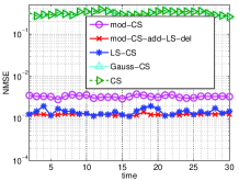
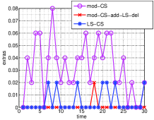
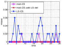
(a) $r=3/3,d=3,M=dr=3$

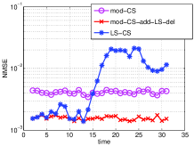
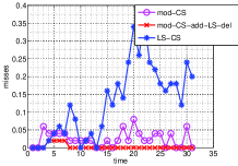
(b) $r=3/4,d=4,M=dr=3$

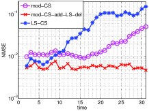
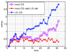
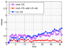
(c) $r=2/4,d=4,M=dr=2$

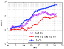
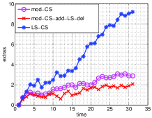
(d) $r=2/5,d=5,M=dr=2$

Figure 1: Normalized MSE (NMSE), number of extras and number of misses over time for modified-CS, modified-CS with add-LS-del and LS-CS. In all cases, NMSE for CS was more than 20% in all cases (plotted only in (a)).

VI Simulation Results

We compared modified-CS (mod-cs), modified-CS with Add-LS-Del (mod-cs-add-del), LS-CS and simple CS for a few different choices of $r$. In all cases, we used Signal Model 1 with $m=200$, $S_{0}=20$, $S_{a}=2$, $n=59$ and $w_{t}\sim^{i.i.d.}uniform(-c,c)$ with $c=0.1266$. The specific generative model that we used is specified in Appendix -A and also briefly discussed in Sec. II. The measurement matrix was random-Gaussian. We averaged over 50 simulations. In all cases, we set the addition threshold, $\alpha_{add}$, to be at the noise level - we set it to $c/2$. Assuming that the LS step after addition gives a fairly accurate estimate of the nonzero values, one can set the deletion threshold, $\alpha_{del}$, to a larger value of $r/2$ and still ensure that there are no (or very few) false deletions. Larger deletion threshold ensures that all (or most) of the false additions and removals get deleted. Modified-CS used a single threshold, $\alpha$, somewhere in between $\alpha_{add}$ and $\alpha_{del}$. We set $\alpha=((c/2)+(r/2))/2$.

In Fig. 1, we show two sets of plots: $r=1$, $d=3$ ($M=dr=3$) in 1(a) and $r=0.5$, $d=4$ ($M=dr=2$) in 1(c). Normalized MSE (NMSE), average number of extras (mean of $|{\hat{N}}_{t}\setminus N_{t}|$ over the 50 simulations) and average number of misses (mean of $|N_{t}\setminus{\hat{N}}_{t}|$) are plotted in the left, middle and right columns respectively. Notice that when the support size is $S_{0}=20$, $n=59$ is too small for CS to work and hence in all cases, the NMSE of CS was more than 20%. We show its NMSE only in 1(a).

When $r=1$, all of mod-cs, mod-cs-add-del and ls-cs are stable. Mod-cs-add-del uses a better support estimation method (add-LS-del) and thus its extras and misses are both much smaller than those of mod-cs (in this case, it is possible that if we experimented with many different threshold choices, mod-cs error could be made smaller). As a result its reconstruction error is also stable at a smaller value. In this case, since $r$ is large enough, LS-CS (which also uses add-LS-del) has similar error to that of Mod-cs-add-del. When $r$ is reduced to 0.75, it becomes too small for LS-CS and so LS-CS becomes unstable. LS-CS stability is discussed in Sec. V. As we explain there, due to the CS-residual step, LS-CS needs a larger $r$ for stability. When $r$ is reduced to 0.5, mod-CS also becomes unstable. But mod-cs-add-del is still stable. Mod-CS uses one threshold and hence as explained after Theorem 1, it needs a larger $r$ for stability than mod-cs-add-del. Finally if we reduce $r$ to 0.4, all three became unstable.

VII Conclusions

We showed the “stability” of modified-CS and its improved version, modified-CS with add-LS-Del, and of LS-CS for signal sequence reconstruction, under mild assumptions. By “stability” we mean that the number of misses from the current support estimate and the number of extras in it remain bounded by a time-invariant value at all times. The result is meaningful when the bound is small compared to the support size.

-A A generative model for Signal Model 1

To help understand the model better (and also to simulate it), we describe here one plausible generative model that satisfies its required assumptions. This assumes that every element gets added to the support at magnitude $r$ and keeps increasing until it reaches magnitude $M$. Similarly, every element that began decreasing keeps decreasing until it becomes zero and gets removed from the support. We keep the signs of the elements the same except when the element first gets added (at that time, can set the sign to $\pm 1$ with equal probability).

To specify the generative model, first define

Definition 5

Define

1. Increasing set, $\text{Inc}_{t}:={\cal I}_{t}(1)\cup{\cal I}_{t}(2)\dots\cup{\cal I}_{t}(d-1)$

2. Decreasing set, $\text{Dec}_{t}:={\cal D}_{t}(1)\cup{\cal D}_{t}(2)\dots\cup{\cal D}_{t}(d-1)$

3. Constant set, $\text{Con}_{t}:=\{i:|x_{t,i}|=M\}$. Clearly $\text{Con}_{t}=N_{t}\setminus(\text{Inc}_{t}\cup\text{Dec}_{t})$.

The generative model is as follows. At each $t>0$,

1. Update the magnitudes for elements of the previous increasing, decreasing and constant sets.

   $$(x_{t})_{\text{Inc}_{t-1}} = [|(x_{t-1})_{\text{Inc}_{t-1}}|+r]\ \text{sgn}((x_{t-1})_{\text{Inc}_{t-1}})$$

   $$(x_{t})_{\text{Dec}_{t-1}} = [|(x_{t-1})_{\text{Dec}_{t-1}}|-r]\ \text{sgn}((x_{t-1})_{\text{Dec}_{t-1}})$$

   $$(x_{t})_{\text{Con}_{t-1}} = (x_{t-1})_{\text{Con}_{t-1}}$$ (20)

   where $\text{sgn}(z)$ is a vector containing the signs of each element of $z$.

2. Select the newly added set, ${\cal I}_{t}(1)\subseteq N_{t-1}^{c}$, of size $S_{a}$ uniformly at random. Similarly select the new set of decreasing elements, ${\cal D}_{t}(d-1)\subseteq\text{Con}_{t-1}$ of size $S_{a}$ uniformly at random. Set their values as:

   $$(x_{t})_{{\cal I}_{t}(1)} = r\ \underline{s}$$

   $$(x_{t})_{{\cal D}_{t}(d-1)} = (d-1)r\ \text{sgn}((x_{t-1})_{{\cal D}_{d-1}})$$ (21)

   where $\underline{s}$ is an $S_{a}\times 1$ signs’ vector in which each element is $+1$ or $-1$ with probability $1/2$.

3. Compute:

   $${\cal I}_{t}(d) = \{i\in\text{Inc}_{t-1}:|(x_{t-1})_{i}|=(d-1)r\}$$

   $${\cal D}_{t}(0) = \{i\in\text{Dec}_{t-1}:|(x_{t-1})_{i}|=r\}$$ (22)

   and update the increasing, decreasing and constant sets:

   $$\text{Inc}_{t} = \text{Inc}_{t-1}\cup{\cal I}_{t}(1)\setminus{\cal I}_{t}(d)$$

   $$\text{Dec}_{t} = \text{Dec}_{t-1}\cup{\cal D}_{t}(d-1)\setminus{\cal D}_{t}(0)$$

   $$\text{Con}_{t} = \text{Con}_{t-1}\cup{\cal I}_{t}(d)\setminus{\cal D}_{t}(d-1)$$

   $$N_{t} = \text{Inc}_{t}\cup\text{Dec}_{t}\cup\text{Con}_{t}$$ (23)

-B Appendix: Proof of Theorem 1

We prove the first claim by induction. Using condition 4 of the theorem, the claim holds for $t=0$. This proves the base case. For the induction step, assume that the claim holds at $t-1$, i.e. $|{\tilde{\Delta}}_{e,t-1}|=0$, $|{\tilde{T}}_{t-1}|\leq S_{0}$, and ${\tilde{\Delta}}_{t-1}\subseteq{\cal S}_{t-1}(2)$ so that $|{\tilde{\Delta}}_{t-1}|\leq 2S_{a}$. Using this assumption we prove that the claim holds at $t$. In the proof, we use the following facts often: (a) ${\cal R}_{t}\subseteq N_{t-1}$ and ${\cal A}_{t}\subseteq N_{t-1}^{c}$, (b) $N_{t}=N_{t-1}\cup{\cal A}_{t}\setminus{\cal R}_{t}$, and (c) if two sets $B,C$ are disjoint, then, $(D\cap B^{c})\cup C=D\cup C\setminus B$ for any set $D$.

We first bound $|T_{t}|$, $|\Delta_{e,t}|$ and $|\Delta_{t}|$. Since $T_{t}={\tilde{T}}_{t-1}$, so $|T_{t}|\leq S_{0}$. Since $\Delta_{e,t}={\hat{N}}_{t-1}\setminus N_{t}={\hat{N}}_{t-1}\cap[(N_{t-1}^{c}\cap{\cal A}_{t}^{c})\cup{\cal R}_{t}]\subseteq{\tilde{\Delta}}_{e,t-1}\cup{\cal R}_{t}={\cal R}_{t}$. The last equality follows since $|{\tilde{\Delta}}_{e,t-1}|=0$. Thus $|\Delta_{e,t}|\leq|{\cal R}_{t}|=S_{a}$. Now consider $|\Delta_{t}|$. Notice that $\Delta_{t}=N_{t}\setminus{\hat{N}}_{t-1}=(N_{t-1}\cap{\hat{N}}_{t-1}^{c}\cap{\cal R}_{t}^{c})\cup({\cal A}_{t}\cap{\cal R}_{t}^{c}\cap{\hat{N}}_{t-1}^{c})=({\tilde{\Delta}}_{t-1}\cap{\cal R}_{t}^{c})\cup({\cal A}_{t}\cap{\hat{N}}_{t-1}^{c})\subseteq({\cal S}_{t-1}(2)\cap{\cal R}_{t}^{c})\cup{\cal A}_{t}={\cal S}_{t-1}(2)\cup{\cal A}_{t}\setminus{\cal R}_{t}$. The second last equality uses ${\tilde{\Delta}}_{t-1}\subseteq{\cal S}_{t-1}(2)$. Since ${\cal R}_{t}$ is a subset of ${\cal S}_{t-1}(2)$ and ${\cal A}_{t}$ is disjoint with ${\cal S}_{t-1}(2)$, thus $|\Delta_{t}|\leq|{\cal S}_{t-1}(2)|+|{\cal A}_{t}|-|{\cal R}_{t}|=2S_{a}+S_{a}-S_{a}=2S_{a}$.

Next we bound $|{\tilde{\Delta}}_{t}|$, $|{\tilde{\Delta}}_{e,t}|$ and $|{\tilde{T}}_{t}|$. Consider the support estimation step. Apply the first claim of Lemma 2 with $S_{N}=S_{0}$, $S_{\Delta_{e}}=S_{a}$, $S_{\Delta}=2S_{a}$, and $b_{1}=2r$. Since conditions 2 and 3 of the theorem hold, all elements of $N_{t}$ with magnitude equal or greater than $2r$ will get detected. Thus, ${\tilde{\Delta}}_{t}\subseteq{\cal S}_{t}(2)$. Apply the second claim of the lemma. Since conditions 2 and 1 hold, all zero elements will get deleted and there will be no false detections, i.e. $|{\tilde{\Delta}}_{e,t}|=0$. Finally using $|{\tilde{T}}_{t}|\leq|N_{t}|+|{\tilde{\Delta}}_{e,t}|$, $|{\tilde{T}}_{t}|\leq S_{0}$.

-C Appendix: Proof of Theorem 2

We prove the first claim of the theorem by induction. Using condition 4 of the theorem, the claim holds for $t=0$. This proves the base case. For the induction step, assume that the claim holds at $t-1$, i.e. $|{\tilde{\Delta}}_{e,t-1}|=0$, $|T_{t-1}|\leq S_{0}$, and ${\tilde{\Delta}}_{t-1}\subseteq{\cal S}_{t-1}(2)$ so that $|{\tilde{\Delta}}_{t-1}|\leq 2S_{a}$. Using the induction assumption, we prove that the claim holds at $t$. In the proof, we will use the following facts often: ${\cal R}_{t}\subseteq N_{t-1}$, ${\cal A}_{t}\subseteq N_{t-1}^{c}$ and $N_{t}=N_{t-1}\cup{\cal A}_{t}\setminus{\cal R}_{t}$. Also, if two sets $B,C$ are disjoint, then, $(D\cap B^{c})\cup C=D\cup C\setminus B$ for any set $D$.

Since $T_{t}=T_{t-1}$, so $|T_{t}|\leq S_{0}$. Since $\Delta_{e,t}={\hat{N}}_{t-1}\setminus N_{t}={\hat{N}}_{t-1}\cap[(N_{t-1}^{c}\cap{\cal A}_{t}^{c})\cup{\cal R}_{t}]\subseteq{\tilde{\Delta}}_{e,t-1}\cup{\cal R}_{t}={\cal R}_{t}$. The last equality follows since $|{\tilde{\Delta}}_{e,t-1}|=0$. Thus $|\Delta_{e,t}|\leq|{\cal R}_{t}|=S_{a}$. Next we bound $|\Delta_{t}|$. Note that $\Delta_{t}=N_{t}\setminus{\hat{N}}_{t-1}=(N_{t-1}\cap{\hat{N}}_{t-1}^{c}\cap{\cal R}_{t}^{c})\cup({\cal A}_{t}\cap{\cal R}_{t}^{c}\cap{\hat{N}}_{t-1}^{c})=({\tilde{\Delta}}_{t-1}\cap{\cal R}_{t}^{c})\cup({\cal A}_{t}\cap{\hat{N}}_{t-1}^{c})\subseteq({\cal S}_{t-1}(2)\cap{\cal R}_{t}^{c})\cup{\cal A}_{t}={\cal S}_{t-1}(2)\cup{\cal A}_{t}\setminus{\cal R}_{t}$. Since ${\cal R}_{t}$ is a subset of ${\cal S}_{t-1}(2)$ and ${\cal A}_{t}$ is disjoint with ${\cal S}_{t-1}(2)$, thus $|\Delta_{t}|\leq|{\cal S}_{t-1}(2)|+|{\cal A}_{t}|-|{\cal R}_{t}|=2S_{a}+S_{a}-S_{a}$.

Consider the detection step. There are at most $S_{a}$ false detects (from condition 1a) and thus $|{\tilde{\Delta}}_{e,{\text{add}},t}|\leq|\Delta_{e,t}|+S_{a}\leq 2S_{a}$. Thus $|T_{{\text{add}},t}|\leq|N_{t}|+|{\tilde{\Delta}}_{e,{\text{add}},t}|\leq S_{0}+2S_{a}$. Next we bound $|\Delta_{{\text{add}},t}|$. Using the above discussion, $\Delta_{t}\subseteq{\cal S}_{t-1}(2)\cup{\cal A}_{t}\setminus{\cal R}_{t}$. Using (3) for $j=2$, the RHS equals ${\cal S}_{t}(2)\cup{\cal I}_{t}(2)\setminus{\cal D}_{t}(1)$. Apply Lemma 3 with $S_{N}=S_{0}$, $S_{\Delta_{e}}=S_{a}$, $S_{\Delta}=2S_{a}$, and with $b_{1}=2r$ (so that $\Delta_{1}\subseteq{\cal I}_{t}(2)$). Since conditions 2 and 3 of the theorem hold, all the undetected elements of ${\cal I}_{t}(2)$ will definitely get detected at time $t$. Thus $\Delta_{{\text{add}},t}\subseteq{\cal S}_{t}(2)\setminus{\cal D}_{t}(1)$. Since ${\cal D}_{t}(1)\subseteq{\cal S}_{t}(2)$, so $|\Delta_{{\text{add}},t}|\leq|{\cal S}_{t}(2)|-|{\cal D}_{t}(1)|=S_{a}$.

Consider the deletion step. Apply Lemma 5 with $S_{T}=S_{0}+2S_{a}$, $S_{\Delta}=S_{a}$. Since condition 2a holds, $\delta_{S_{0}+2S_{a}}<1/2$. Since $\Delta_{{\text{add}},t}\subseteq{\cal S}_{t}(2)\setminus{\cal D}_{t}(1)$, so $\|x_{\Delta_{{\text{add}}}}\|\leq\sqrt{S_{a}}r$. Since condition 1b also holds, all elements of ${\tilde{\Delta}}_{e,{\text{add}},t}$ will get deleted. Thus $|{\tilde{\Delta}}_{e,t}|=0$. Thus $|{\tilde{T}}_{t}|\leq|N_{t}|+|{\tilde{\Delta}}_{e,t}|\leq S_{0}$. Next, we bound $|{\tilde{\Delta}}_{t}|$. Apply Lemma 4 with $S_{T}=S_{0}+2S_{a}$, $S_{\Delta}=S_{a}$, $b_{1}=2r$. Since $\Delta_{{\text{add}},t}\subseteq{\cal S}_{t}(2)\setminus{\cal D}_{t}(1)$, so $\|x_{\Delta_{{\text{add}}}}\|\leq\sqrt{S_{a}}r$. By Lemma 4, to ensure that all elements of $T_{{\text{add}},t}$ with magnitude greater than or equal to $b_{1}=2r$ do not get falsely deleted, we need $\delta_{S_{0}+2S_{a}}<1/2$ and $2r>\alpha_{del}+\sqrt{2}\epsilon+2\theta_{S_{0}+2S_{a},S_{a}}\sqrt{S_{a}}r$. From condition 1b, $\alpha_{del}=\sqrt{2}\epsilon+2\theta_{S_{0}+2S_{a},S_{a}}\sqrt{S_{a}}r$. Thus, we need $\delta_{S_{0}+2S_{a}}<1/2$ and $2r>2(\sqrt{2}\epsilon+2\theta_{S_{0}+2S_{a},S_{a}}\sqrt{S_{a}}r)$. $\delta_{S_{0}+2S_{a}}<1/2$ holds since condition 2a holds. The second condition holds since condition 2b and condition 3 ($r\geq G_{2}$) hold. Thus, we can ensure that all elements of $T_{{\text{add}},t}$ with magnitude greater than or equal to $b_{1}=2r$ do not get falsely deleted. But nothing can be said about the elements smaller than $2r$. In the worst case ${\tilde{\Delta}}_{t}$ may contain all of these elements, i.e. it may be equal to ${\cal S}_{t}(2)$. Thus, ${\tilde{\Delta}}_{t}\subseteq{\cal S}_{t}(2)$ and so $|{\tilde{\Delta}}_{t}|\leq 2S_{a}$.

This finishes the proof of the first claim. To prove the second and third claims for any $t>0$: use the first claim for $t-1$ and the arguments from the paragraphs above to show that the second and third claim hold for $t$. The fourth claim follows directly from the first claim and fact 4 of Proposition 2 (applied with $x\equiv\hat{x}_{t}$, $T\equiv{\tilde{T}}_{t}$, $\Delta\equiv{\tilde{\Delta}}_{t}$). The fifth claim follows directly from the second claim and Corollary 1.

-D Appendix: Generalized version of Theorem 2

Theorem 4 (Stability of modified-CS with add-LS-del)

Assume Signal Model 1 and $\|w_{t}\|\leq\epsilon$. Let $e_{t}:=(x_{t}-\hat{x}_{{\text{add}},t})_{T_{{\text{add}},t}}$. Assume that $\|e_{t}\|_{\infty}\leq\|e_{t}\|/\sqrt{S_{a}}$ at all $t$ (the LS step error is spread out enough). If for some $1\leq d_{0}\leq d$,

1. (addition and deletion thresholds)

   1. $\alpha_{add}$ is large enough so that there are at most $f$ false additions per unit time,

   2. $\alpha_{del}=\sqrt{\frac{2}{S_{a}}}\epsilon+2k_{3}\theta_{S_{0}+S_{a}+f,k_{2}}r$,

2. (support size, support change rate) $S_{0},S_{a}$ satisfy

   1. $\delta_{S_{0}+S_{a}(1+k_{1})}<(\sqrt{2}-1)/2$ ,

   2. $\delta_{S_{0}+S_{a}+f}<1/2$,

   3. $\theta_{S_{0}+S_{a}+f,k_{2}}<\frac{1}{2}\frac{d_{0}}{4k_{3}}$,

3. (new element increase rate) $r\geq\max(G_{1},G_{2})$, where

   $$G_{1} \triangleq \frac{\alpha_{add}+8.79\epsilon}{d_{0}}$$

   $$G_{2} \triangleq \frac{2\sqrt{2}\epsilon}{\sqrt{S_{a}}(d_{0}-4k_{3}\theta_{S_{0}+S_{a}+f,k_{2}})}\ \ \ \ \ \ \$$ (24)

4. (initial time) at $t=0$, $n_{0}$ is large enough to ensure that ${\tilde{\Delta}}\subseteq{\cal S}_{0}(d_{0})$, $|{\tilde{\Delta}}|\leq(2d_{0}-2)S_{a}$, $|{\tilde{\Delta}}_{e}|=0$, $|{\tilde{T}}|\leq S_{0}$,

where

$$k_{1} \triangleq \max(1,2d_{0}-2)$$

$$k_{2} \triangleq \max(0,2d_{0}-3)$$

$$k_{3} \triangleq \sqrt{\sum_{j=1}^{d_{0}-1}j^{2}+\sum_{j=1}^{d_{0}-2}j^{2}}$$ (25)

then, at all $t\geq 0$,

1. $|{\tilde{T}}|\leq S_{0}$, $|{\tilde{\Delta}}_{e}|=0$, and ${\tilde{\Delta}}\subseteq{\cal S}_{t}(d_{0})$ and so $|{\tilde{\Delta}}|\leq(2d_{0}-2)S_{a}$,

2. $|T|\leq S_{0}$, $|\Delta_{e}|\leq S_{a}$, and $|\Delta|\leq k_{1}$,

3. $|T_{\text{add}}|\leq S_{0}+S_{a}+f$, $|\Delta_{e,{\text{add}}}|\leq S_{a}+f$, and $|{\tilde{\Delta}}_{\text{add}}|\leq k_{2}$

4. $\|x_{t}-\hat{x}_{t}\|\leq\sqrt{2}\epsilon+k_{3}\sqrt{S_{a}}(2\theta_{S_{0},(2d_{0}-2)S_{a}}+1)r$

5. $\|x_{t}-\hat{x}_{t,modcs}\|\leq C_{1}(S_{0}+S_{a}+k_{1})\epsilon\leq 8.79\epsilon$.

-E Proof of Lemma 9

From Lemma 8, if $\|w\|\leq\epsilon$, $\delta_{2|\Delta|}<\sqrt{2}-1$ and $\delta_{|T|}<1/2$, then $\|x-\hat{x}_{CSres}\|\leq C^{\prime}(|T|,|\Delta|)\epsilon+\theta_{|T|,|\Delta|}C^{\prime\prime}(|T|,|\Delta|)\|x_{\Delta}\|$. Using the fact that $\|x_{\Delta}\|\leq\sqrt{|\Delta_{1}|}b+\|x_{\Delta_{2}}\|$; fact 1 of Proposition 2; and the fact that for all $i\in\Delta_{1}$, $|x_{i}|\geq\gamma b$, we can conclude that all $i\in\Delta_{1}$ will get detected if $\delta_{2|\Delta|}<(\sqrt{2}-1)/2$, $\delta_{|T|}<1/2$ and $\alpha_{add}+C^{\prime}\epsilon+\theta C^{\prime\prime}\|x_{\Delta_{2}}\|+\theta C^{\prime\prime}\sqrt{|\Delta_{1}|}b<\gamma b$. Using $\|x_{\Delta_{2}}\|\leq\kappa b$ and $|\Delta_{1}|\leq S_{\Delta_{1}}$, this last inequality holds if $\theta C^{\prime\prime}\leq{\gamma}/{2(\sqrt{S_{\Delta_{1}}}+\kappa)}$ and $\frac{\alpha_{add}+C^{\prime}\epsilon}{\gamma-\theta C^{\prime\prime}(\sqrt{S_{\Delta_{1}}}+\kappa)}<b$. Since we only know that $|T|\leq S_{T}$, $|\Delta|\leq S_{\Delta}$, $|\Delta_{1}|\leq S_{\Delta_{1}}$ and $\|x_{\Delta_{2}}\|\leq\kappa$, we need the above four inequalities to hold for all values of $|T|,|\Delta|,|\Delta_{1}|,\|x_{\Delta_{2}}\|$ satisfying these upper bounds. This leads to the conclusion of the lemma. Notice that the LHS’s of all the required inequalities, except the last one, are non-decreasing functions of $|\Delta|,|T|,|\Delta_{1}|$ and thus the lemma just uses their upper bounds. The LHS of the last one is non-decreasing in $|T|,|\Delta_{1}|,\|x_{\Delta_{2}}\|$, but is not monotonic in $|\Delta|$ (since $C^{\prime}(|T|,|\Delta|)$ is not monotonic in $|\Delta|$). Hence we explicitly maximize over $|\Delta|\leq S_{\Delta}$. $\blacksquare$

References

- [1] N. Vaswani and W. Lu, “Modified-cs: Modifying compressive sensing for problems with partially known support,” IEEE Trans. Sig. Proc., 2010 (to appear), shorter version in ISIT 2009.
- [2] W. Lu and N. Vaswani, “Modified bpdn for noisy compressive sensing with partially known support,” in ICASSP, 2010.
- [3] N. Vaswani, “Least Squares CS-residual (LS-CS): Compressive Sensing on Least Squares residual,” IEEE Trans. Sig. Proc., August 2010.
- [4] N. Vaswani, “Kalman filtered compressed sensing,” in ICIP, 2008.
- [5] N. Vaswani, “Analyzing least squares and kalman filtered compressed sensing,” in ICASSP, 2009.
- [6] D. Angelosante, G.B. Giannakis, and E. Grossi, “Compressed sensing of time-varying signals,” in DSP, 2009.
- [7] M. S. Asif and J. Romberg, “Dynamic updating for sparse time varying signals,” in CISS, 2009.
- [8] A. Carmi, P. Gurfil, and D. Kanevsky, “A simple method for sparse signal recovery from noisy observations using kalman filtering,” in IBM Technical report, December 2008.
- [9] R. von Borries, C. J. Miosso, and C. Potes, “Compressed sensing using prior information,” in IEEE Intl. Workshop on Computational Advances in Multi-Sensor Adaptive Processing (CAMSAP), 2007.
- [10] A. Khajehnejad, W. Xu, A. Avestimehr, and B. Hassibi, “Weighted l1 minimization for sparse recovery with prior information,” in ISIT, 2009.
- [11] D. Needell and J.A. Tropp., “Cosamp: Iterative signal recovery from incomplete and inaccurate samples,” Appl. Comp. Harmonic Anal., vol. 26, pp. 301–321, 2008.
- [12] E. Candes and T. Tao, “The dantzig selector: statistical estimation when p is much larger than n,” Annals of Statistics, vol. 35 (6), 2007.
- [13] L. Jacques, “A short note on compressed sensing with partially known signal support,” ArXiv preprint 0908.0660, 2009.
- [14] E. Candes, “The restricted isometry property and its implications for compressed sensing,” Compte Rendus de l’Academie des Sciences, Paris, Serie I, pp. 589–592, 2008.
- [15] J. A. Tropp, “Just relax: Convex programming methods for identifying sparse signals,” IEEE Trans. Info. Th., pp. 1030–1051, March 2006.