Gravitating fluids with Lie symmetries

Abstract

We analyse the underlying nonlinear partial differential equation which arises in the study of gravitating flat fluid plates of embedding class one. Our interest in this equation lies in discussing new solutions that can be found by means of Lie point symmetries. The method utilised reduces the partial differential equation to an ordinary differential equation according to the Lie symmetry admitted. We show that a class of solutions found previously can be characterised by a particular Lie generator. Several new families of solutions are found explicitly. In particular we find the relevant ordinary differential equation for all one-dimensional optimal subgroups; in several cases the ordinary differential equation can be solved in general. We are in a position to characterise particular solutions with a linear barotropic equation of state.

PACS numbers: 02.30.Gp, 02.30.Jr, 04.20.Jb

1 Introduction

The local isometric embedding of four-dimensional Riemannian manifolds $M_{4}$ in higher dimensional flat pseudo-Euclidean spaces $E_{N}(N\leq 10)$ is important for several applications in general relativity. For the basic theory and general results pertinent to embeddings the reader is referred to Stephani et al (2003). The invariance of the embedding class naturally generates a classification scheme for all solutions of the field equations in terms of their embedding class. The embedding class $p$ is the minimum number of extra dimensions of the Riemannian manifold $M_{4}$, ie. $p=N-4$. Exact solutions have been found by the method of embedding in particular spacetimes for simple cases of low embedding class. Some of these exact solutions may not be easily found using other methods and techniques. For example the embedding method has been utilised to find all conformally flat perfect fluid solutions, in embedding class $p=1$, of Einstein’s field equations (Krasinki 1997, Stephani 1967a, Stephani 1967b). We point out that embedding of four-dimensional Riemannian manifolds in higher dimensional spacetimes with arbitrary Ricci tensors has been investigated by several authors. The physical motivation here is to understand the nature of physics in higher dimensions; the modern view is that the Riemannian manifold $M_{4}$ is a hypersurface in the higher dimensional bulk in the brane world scenario and other higher dimensional themes (Dahia and Romero 2002a, Dahia and Romero 2002b, Dahia et al 2008).

Gupta and Sharma (1996) have generated a relativistic model in higher dimensions describing gravitating fluid plates. Advantages of this model are that it is easy to interpret the physical features using embedding in higher dimensions and the underlying differential equation governing the gravitational dynamics is tractable. This model is expanding and not conformally flat. A plane symmetric metric in four-dimensional spacetimes $M_{4}$ given by

$${\rm d}s^{2}=-{\rm d}r^{2}-t^{2}({\rm d}\theta^{2}+\theta^{2}{\rm d}\phi^{2})+(1+2\dot{V}){\rm d}t^{2}+2V^{\prime}{\rm d}r{\rm d}t$$ (1)

is embedded in the five-dimensional pseudo-Euclidean space $E_{5}$ with metric

$${\rm d}s^{2}=-({\rm d}z^{1})^{2}-({\rm d}z^{2})^{2}-({\rm d}z^{3})^{2}+({\rm d}z^{4})^{2}-({\rm d}z^{5})^{2}.$$ (2)

This embedding is achieved by setting

$$z^{1} = t\theta\cos\phi$$ (3a)

$$z^{2} = t\theta\sin\phi$$ (3b)

$$z^{3} = \frac{\theta^{2}}{2}t+V$$ (3c)

$$z^{4} = t\left(\frac{\theta^{2}}{2}+1\right)+V$$ (3d)

$$z^{5} = r$$ (3e)

where $V=V(r,t)$ is an arbitrary function.

Consequently this model has embedding class $p=1$ which allows both conformally flat and nonconformally flat fluid distributions. The solutions admitted may be geodesic or accelerating. For a nonzero conformal (Weyl) tensor a partial differential equation has to be satisfied. This pivotal equation governs the evolution of the system and a particular class of solutions was identified by Gupta and Sharma (1996) by inspection. A detailed analysis of the pivotal equation shows that other classes of solution are possible which contain the Gupta and Sharma (1996) models as a special case.

Our intention is to systematically study the pivotal equation and to obtain a deeper insight into the nature of solutions permitted using the Lie analysis of differential equations. In $\S 2$ we discuss the fundamental partial differential equation that governs the gravitational behaviour of the model, and present known solutions. An outline of the basic features of the Lie symmetry analysis is given in $\S 3$. We regain the Gupta and Sharma (1996) models using the relevant Lie generator in $\S 4$. In $\S 5$ we systematically study the group invariant solutions admitted by the fundamental equation. The partial differential equation is reduced to an ordinary differential equation for each element of the optimal system. The integrability of the ordinary differential equation is considered in each case and exact solutions are identified. The physical features of the model are discussed in $\S 6$ and equations of state are found for particular solutions. Some brief concluding comments are made in $\S 7$.

2 The model

The embedding of the four-dimensional Riemannian metric (1) into the five-dimensional flat metric (2) leads to a differential equation that is central to the model. Gupta and Sharma (1996) show that the pivotal equation is

$$-V_{tt}V_{rr}+V_{rt}{}^{2}+\frac{1}{t}\left[(1+2V_{t})V_{rr}-V_{tt}-2V_{rt}V_{r}\right]$$

$$+\frac{1}{t^{2}}\left[1+2V_{t}+V_{r}{}^{2}\right]=0$$ (3d)

where subscripts denotes partial differentiation. This is a nonlinear equation in $V$ and difficult to solve. We need to explicitly solve (3d) to describe the gravitational dynamics.

To demonstrate a class of solutions to (3d), Gupta and Sharma (1996) made the following assumption

$$V=C\left(\frac{f(r)}{t}+h(t)\right)+C_{1}$$ (3e)

where $C$ and $C_{1}$ are arbitrary constants. Then (3d) reduces to the separable form

$$4f-\frac{4Cf_{r}{}^{2}}{Cf_{rr}+1}=t^{2}\left[\frac{1}{C}-th_{tt}+2h_{t}\right]=\alpha$$ (3f)

where $\alpha$ is the constant of separability. It is possible to solve the equation (3f) in terms of $t$ explicitly as

$$h=-\frac{\alpha}{4t}-\frac{t}{2C}-\frac{\alpha_{1}t^{3}}{3}+\alpha_{2}$$ (3g)

and to provide four solutions to the equation in terms of $r$, viz

$$f = \frac{1}{2m^{2}C}\sin X+\frac{1}{2m^{2}C}+\frac{\alpha}{4}$$ (3ha)

$$f = \frac{\alpha}{4}$$ (3hb)

$$f = \frac{1}{2C}(r+\beta)^{2}+\frac{\alpha}{4}$$ (3hc)

$$f = \frac{1}{2m^{2}C}\cosh X-\frac{1}{2m^{2}C}+\frac{\alpha}{4}$$ (3hd)

where we have set $X=\sqrt{2}mr+m_{0}$ and $\alpha_{1},\alpha_{2},\beta,m$ and $m_{0}$ are arbitrary constants.

Equations (3g) and (3ha)–(3hd) are then combined to provide solutions to the original equation (3d), viz

$$V = \frac{1}{2m^{2}t}\sin X+\frac{1}{2m^{2}t}-\frac{t}{2}-\frac{kt^{3}}{3}+k_{1}$$ (3hia)

$$V = -\frac{t}{2}-\frac{kt^{3}}{3}+k_{1}$$ (3hib)

$$V = \frac{1}{2t}(r+\beta)^{2}-\frac{t}{2}-\frac{kt^{3}}{3}+k_{1}$$ (3hic)

$$V = \frac{1}{2m^{2}t}\cosh X-\frac{1}{2m^{2}t}-\frac{t}{2}-\frac{kt^{3}}{3}+k_{1}$$ (3hid)

where $k=C\alpha_{1}$ and $k_{1}=C\alpha_{2}$. Thus the assumption (3e) leads to a simple class of solutions (3hia)–(3hid) which are written in terms of elementary functions. As an aside we observe that $\alpha$ does not appear in the solutions (3hia)–(3hid). Thus the constant of separability $\alpha$ can be taken to be zero, and $C$ can be taken to be unity with no loss of generality. Indeed as we shall demonstrate later, our Lie analysis obviates the need for the introduction of $\alpha$ and $C$.

We will show that, while (3e) is an ad hoc assumption, the reason for its feasibility lies in the group theoretic properties of (3d). Utilising the full group properties of (3d) we can provide further solutions to complement (3hia)–(3hid).

3 Lie analysis

The basic feature of Lie analysis requires the determination of the one–parameter (${\varepsilon}$) Lie group of transformations

$$\bar{t} = t+{\varepsilon}\tau(t,r,u)+O({\varepsilon}^{2})$$

$$\bar{r} = r+{\varepsilon}\xi(t,r,u)+O({\varepsilon}^{2})$$ (3hij)

$$\bar{u} = u+{\varepsilon}\eta(t,r,u)+O({\varepsilon}^{2})$$

that leaves the solution set of a differential equation invariant. (The full details can be found in a number of excellent texts (Bluman and Kumei 1989, Olver 1993).) In order to obtain (3hij) we need to determine their “generator”

$$G=\tau\frac{\partial\ }{\partial t}+\xi\frac{\partial\ }{\partial r}+\eta\frac{\partial\ }{\partial u}$$ (3hik)

(also called a symmetry of the differential equation) which is a set of vector fields.

The determination of these generators is a straight forward, albeit tedious process. Fortunately, a number of computer algebra packages are available to aid the practitioner (Hereman 1994). While some modern packages have been developed (Dimas and Tsoubelis 2005, Cheviakov 2007), we have found the package PROGRAM LIE (Head 1993) to be the most useful in practice. Indeed it is quite remarkable how accomplished such an old package is – it often outperforms its modern counterparts!

Utilising PROGRAM LIE, we can demonstrate that (3d) admits the following Lie point symmetries/vector fields:

$$G_{1} = \frac{\partial\ }{\partial V}$$ (3hila)

$$G_{2} = \frac{\partial\ }{\partial r}$$ (3hilb)

$$G_{3} = t^{3}\frac{\partial\ }{\partial V}$$ (3hilc)

$$G_{4} = t\frac{\partial\ }{\partial r}+r\frac{\partial\ }{\partial V}$$ (3hild)

$$G_{5} = t\frac{\partial\ }{\partial t}-(V+t)\frac{\partial\ }{\partial V}$$ (3hile)

$$G_{6} = r\frac{\partial\ }{\partial r}+(t+2V)\frac{\partial\ }{\partial V}$$ (3hilf)

with the nonzero Lie bracket relationships

$$\begin{array}[]{lcl}[G_{1},G_{5}]=-G_{1}&&[G_{1},G_{6}]=2G_{1}\\ {}[G_{2},G_{4}]=G_{1}&&[G_{2},G_{6}]=G_{2}\\ {}[G_{3},G_{5}]=-4G_{3}&&[G_{3},G_{6}]=2G_{3}\\ {}[G_{4},G_{5}]=-G_{4}&&[G_{4},G_{6}]=G_{4}\end{array}$$ (3hilm)

for the given fields. As a result, the symmetries (3hila)–(3hilf) form a six–dimensional indecomposable solvable Lie algebra, $L$ (Rand et al, 1988). While $L$ is not nilpotent, its first derived Lie subalgebra $L^{(1)}=<G_{1},G_{2},G_{3},G_{4}>$ is nilpotent and also represents the nilradical of $L$. Further information about such Lie algebras can be found in (Turkowski, 1990).

4 Known solutions

It is possible to demonstrate that the solutions (3hia)–(3hid) are a natural consequence of a subset of these symmetries. If we take the combination

$$\tilde{G} = c_{1}G_{1}+c_{2}G_{2}+G_{5}$$ (3hiln)

$$= t\frac{\partial\ }{\partial t}+(c_{1}-t+c_{2}t^{3}-V)\frac{\partial\ }{\partial V}$$

the partial differential equation (3d) is reduced to the ordinary differential equation

$$UU_{rr}-U_{r}{}^{2}+U=0$$ (3hilo)

as the essential equation governing the gravitational dynamics where $V=c_{1}-\frac{t}{2}+\frac{c_{2}t^{3}}{4}+\frac{U}{t}$.

On comparing (3f) and (3hilo) we can identify the function $f$ with $U$. We are now in a position to make a number of comments relating to the underlying assumption (3e) in the Gupta and Sharma (1996) solutions. We observe that the $t$-dependence arises naturally because of the choice of the symmetry $\tilde{G}$. Thus the temporal dependence is not arbitrary as suggested by the function $h(t)$ in the choice (3e). It is not necessary to solve any differential equation to obtain the form of $h(t)$ given by (3g). In addition, the solutions of (3hilo) are the same as (3ha)–(3hd) with $\alpha=0$ and $C=1$. As stated earlier, the final solutions (3hia)–(3hid) do not include these constants. Thus the Lie symmetry $\tilde{G}$ leads directly to the canonical form of the solution to (3d) without the need to introduce spurious arbitrary functions and parameters.

5 Group invariant solutions

We now seek to utilise the Lie point symmetries in a systematic manner to generate new solutions. These new solutions are termed group invariant solutions as they will be invariant under the group generated by the symmetry used to find them. The advantage of using Lie point symmetries is that we are guaranteed that the variable combinations obtained will always result in an equation in the new variables - no further “consistency” conditions are needed. As we are dealing with a $1+1$ partial differential equation here, we will always be able to find an ordinary differential equation in the new variables defined by the symmetries.

5.1 The optimal system

Given that equation (3d) has the six symmetries (3hila)-(3hilf), we can find group invariant solutions using each symmetry individually, or any linear combination of symmetries. However, taking all possible combinations into account is overly excessive. It turns out (Olver, 1993), that one only need consider a subspace of this vector space. We use the subalgebraic structure of the symmetries (3hila)-(3hilf) of the system (3d) to construct an optimal system of one-dimensional subgroups. Such an optimal system of subgroups is determined by classifying the orbits of the infinitesimal adjoint representation of a Lie group on its Lie algebra obtained by using its infinitesimal generators. All group invariant solutions can be transformed to those obtained via this optimal system. The process is algorithmic and can be found in (Olver 1993). Here we only summarise the final results.

Table 1: One symmetry: generators and odes.

• Generator	Invariants	ode
  $G_{2}$	$y=t$	$yU_{yy}-2U_{y}-1=0$
  	$V=U(t)$
  $G_{3}$	$y=t$	No ode exists
  	$U(t)=r$
  $G_{4}$	$y=t$	$yU_{yy}-2U_{y}-1=0$
  	$V=\frac{r^{2}}{2t}+U(t)$
  $G_{5}$	$y=r$	$UU_{yy}-(U_{y})^{2}+U=0$
  	$V=-\frac{t}{2}+\frac{1}{t}U(r)$

Table 2: One symmetry: pde solutions.

• Generator	Solution to pde
  $G_{2}$	$V=A+\frac{1}{3}Bt^{3}-\frac{t}{2}$
  $G_{3}$	No solution to pde
  $G_{4}$	$V=\frac{r^{2}}{2t}+A+\frac{1}{3}Bt^{3}-\frac{t}{2}$
  $G_{5}$	$V=-\frac{t}{2}+\frac{1}{t}\left[\frac{1}{2m^{2}}(\sin(\sqrt{2}mr+m_{0})+1)\right]$
  	$V=-\frac{t}{2}$
  	$V=-\frac{t}{2}+\frac{1}{t}\left[\frac{1}{2}(r+\beta)^{2}\right]$
  	$V=-\frac{t}{2}+\frac{1}{t}\left[\frac{1}{2m^{2}}(\cosh(\sqrt{2}mr+m_{0})-1)\right]$

In order to obtain group invariant solutions of (3d) explicitly, the optimal system yields only the following symmetry combinations

$$G_{2}=\frac{\partial}{\partial r}$$ (3hilpa)

$$G_{3}=t^{3}\frac{\partial}{\partial V}$$ (3hilpb)

$$G_{4}=t\frac{\partial}{\partial r}+r\frac{\partial}{\partial V}$$ (3hilpc)

$$G_{5}=t\frac{\partial}{\partial t}-(V+t)\frac{\partial}{\partial V}$$ (3hilpd)

$$G_{2}+G_{3}=\frac{\partial}{\partial r}+t^{3}\frac{\partial}{\partial V}$$ (3hilpe)

$$G_{2}+G_{4}=(1+t)\frac{\partial}{\partial r}+r\frac{\partial}{\partial V}$$ (3hilpf)

$$G_{2}+G_{5}=\frac{\partial}{\partial r}+t\frac{\partial}{\partial t}-(V+t)\frac{\partial}{\partial V}$$ (3hilpg)

$$G_{3}+G_{4}=(t^{3}+r)\frac{\partial}{\partial V}+t\frac{\partial}{\partial r}$$ (3hilph)

$$aG_{5}+G_{6}=r\frac{\partial}{\partial r}+(a+1)t\frac{\partial}{\partial t}+\left[(1-a)V-at\right]\frac{\partial}{\partial V}$$ (3hilpi)

$$G_{2}-G_{3}+G_{4}=(t+1)\frac{\partial}{\partial r}+(r-t^{3})\frac{\partial}{\partial V}$$ (3hilpj)

$$G_{2}+G_{3}+G_{4}=(t+1)\frac{\partial}{\partial r}+(t^{3}+r)\frac{\partial}{\partial V}.$$ (3hilpk)

All solutions of (3d) which are obtained via other combinations of point symmetries can be transformed into the solutions obtained from the combinations above. Here, we have also taken into account the fact that (3d) is invariant under the following involutions: $t\rightarrow-t,r\rightarrow-r$ and $V\rightarrow-V$ and so were able to restrict the optimal system further.

It is clear that the optimal system consists of single elements of the Lie algebra, combinations of two elements and combinations of three elements only. We divide our discussion of the solutions based on this separation.

Table 3: Two symmetries: generators and odes.

• Generator	Invariants	ode
  $G_{2}+G_{3}$	$t=y$	$yU_{yy}-2U_{y}-4y^{6}-1=0$
  	$V=rt^{3}+U(t)$
  $G_{2}+G_{4}$	$t=y$	$(1+2y)(-1-2U_{y}+yU_{yy})=0$
  	$V=\frac{r^{2}}{2(1+t)}+U(t)$
  $G_{3}+G_{4}$	$t=y$	$2+y^{4}+4U_{y}-2yU_{yy}=0$
  	$V=rt^{2}+\frac{r^{2}}{2t}+U(t)$
  $G_{2}+G_{5}$	$r=\ln t+y$	$U_{yy}+4U+4UU_{yy}+5U_{y}$
  	$V=-\frac{t}{2}+\frac{1}{t}U(r-\ln t)$	$-4U^{2}_{y}+U_{y}U_{yy}=0$
  $aG_{5}+G_{6}$	$r=yt^{1/(a+1)}$	$-(1+2a)^{2}U^{2}_{y}+y^{2}U_{yy}$
  	$V=-\frac{t}{2}+t^{(1-a)/(1+a)}U(rt^{-1/(1+a)})$	$+2(-1+a)(1+2a)U(1+U_{yy})$
  		$+yU_{y}(2+5a+aU_{yy})=0$

Table 4: Two symmetries: pde solutions.

• Generator	Solution to pde
  $G_{2}+G_{3}$	$V=rt^{3}+A+\frac{1}{3}Bt^{3}+\frac{t^{7}}{7}-\frac{t}{2}$
  $G_{2}+G_{4}$	$V=A\frac{r^{2}}{2(1+t)}+\frac{1}{3}Bt^{3}-\frac{t}{2}$
  $G_{3}+G_{4}$	$V=rt^{2}+\frac{r^{2}}{2t}+A+\frac{1}{3}Bt^{3}+\frac{t^{5}}{20}-\frac{t}{2}$
  $G_{2}+G_{5}$	No solution to pde
  $aG_{5}+G_{6}$	$V=-\frac{t}{2}+\left(B+\frac{1}{2}\left(-\frac{1}{6}e^{A/2}\left(e^{A}-\frac{4r}{t^{2}}\right)^{3/2}+\frac{e^{A}r}{t^{2}}\right)\right)t^{3}$
  	$(a=-\frac{1}{2})$
  	$V=-\frac{t}{2}-\frac{r^{2}}{2t}+\frac{C^{2}r^{6}}{12t^{3}}+\frac{\sqrt{C^{2}r^{4}-4t^{2}}}{3Ct}-\frac{Cr^{4}\sqrt{C^{2}r^{4}-4t^{2}}}{12t^{3}}+D$
  	$(a=1)$

5.2 One generator

In this section we generate solutions to the master equation (3d) when it admits the individual Lie symmetries $G_{2},G_{3},G_{4}$ and $G_{5}$. We do not consider the generators $G_{1}$ and $G_{6}$ as they do not appear in the optimal system (3hilpa)–(3hilpk). The procedure of generating the invariants, the resultant ordinary differential and finally the solution to the partial differential equation is standard. Consequently we do not provide the details of the calculations, instead the relevant results are collated in tabular form.

In table 1 we present the odes that are generated when a single Lie symmetry generator is present. In table 2 we give solutions to the partial differential equation (3d) when it is invariant under a single generator from the optimal system (3hilpa)–(3hilpk). For the generator $G_{3}$ we do not obtain an invariant involving $V$ and so it is not possible to generate an ordinary differential equation. Thus there is no solution possible invariant under $G_{3}$ alone. For the generators $G_{2}$ and $G_{4}$ it is possible to solve the resulting ordinary differential equations and obtain explicit forms for the function $V$ given in table 2. These are new solutions to equation (3d) which have not been obtained previously. For the generator $G_{5}$ we have obtained the ordinary differential equation

$$UU_{yy}-U_{y}{}^{2}+U = 0$$ (3hilpq)

which is of the same form as (3hilo) in $\S 4$. However it is important to observe that the characteristics here are different from $\S 4$. Consequently the solutions $V$ generated by the Lie symmetry $G_{5}$, and listed in table 2, comprise a new class of exact solutions to equation (3d).

Table 5: Three symmetries: generators and odes.

• Generator	Invariants	ode
  $G_{2}+G_{3}+G_{4}$	$t=y$	$y(5+y(9+y(7+y(2+y^{2}(2+y)^{2}))))$
  	$V=\frac{r^{2}}{2(1+t)}+\frac{rt^{3}}{(1+t)}+U(t)$	$-(1+y)^{3}(1+2y)(-2U_{y}+yU_{yy})=-1$
  $G_{2}-G_{3}+G_{4}$	$t=y$	$y(5+y(9+y(7+y(2+y^{2}(2+y)^{2}))))$
  	$V=\frac{r^{2}}{2(1+t)}-\frac{rt^{3}}{(1+t)}+U(t)$	$-(1+y)^{3}(1+2y)(-2U_{y}+yU_{yy})=-1$

Table 6: Three symmetries: pde solutions.

• Generator	Solution to pde
  $G_{2}+G_{3}+G_{4}$	$V=\frac{r^{2}}{2(1+t)}+\frac{rt^{3}}{(1+t)}+A+\frac{1}{8}\left(\frac{3t}{4}-\frac{19t^{2}}{4}+\frac{t^{4}}{2}+\frac{2t^{5}}{5}+\frac{4}{1+t}\right)$
  	$+\frac{1}{8}t^{3}\left((1+B\frac{8}{3})-\frac{3}{8}(1+8t^{3})\log(1+2t)\right)$
  $G_{2}-G_{3}+G_{4}$	$V=\frac{r^{2}}{2(1+t)}+\frac{rt^{3}}{(1+t)}+A+\frac{1}{8}\left(\frac{3t}{4}-\frac{19t^{2}}{4}+\frac{t^{4}}{2}+\frac{2t^{5}}{5}+\frac{4}{1+t}\right)$
  	$+\frac{1}{8}t^{3}\left((1+B\frac{8}{3})-\frac{3}{8}(1+8t^{3})\log(1+2t)\right)$

5.3 Two generators

We now consider the combinations of two generators which arise in the optimal system (3hilpa)–(3hilpk). Table 3 contains the invariants and reduced ode. Table 4 lists the analytic solutions of the pde, containing all cases that we were able to obtain explicit general solutions.

For the generator $G_{2}+G_{5}$, we have not been able to find a solution to the resultant ode which is highly nonlinear. For the generator $aG_{5}+G_{6}$ the resultant ode is nonlinear and difficult to solve in general. However particular solutions can be found for the special parameter values $a=-\frac{1}{2}$ and $a=1$. It is unlikely that the ode will yield closed form solutions for other values of $a$.

Thus we have generated new analytic solutions to (3d) via combinations of two symmetries of (3d) except for one case corresponding to the generator $G_{2}+G_{5}$.

5.4 Three generators

It finally remains to consider the two combinations of three generators $G_{2}+G_{3}+G_{4}$ and $G_{2}-G_{3}+G_{4}$which appear in the optimal system (3hilpa)-(3hilpk). In both cases it is possible to generate the invariants and reduced ode which are presented in table $5$. The explicit solutions of the pde are given in table $6$. Both functions obtained in table $6$ are new solutions to equation (3d).

6 Physical features

We briefly describe the behaviour of the thermodynamic variables corresponding to the spacetime (1). The energy density and the pressure are given by

$$8\pi\rho = \frac{1}{t^{2}P}+\frac{2}{P^{2}}(V_{tt}V_{rr}-V_{rt}{}^{2})$$ (3hilpra)

$$8\pi p = \frac{1}{t^{2}P}$$ (3hilprb)

respectively, where we have set

$$P=1+2V_{t}+V_{r}{}^{2}.$$ (3hilprs)

For many applications in cosmology it is necessary that there exist barotropic equations of state in the form $p=p(\rho)$ (Stephani et al 2003). We find that for the case of a single generator of the optimal system (3hilpa)–(3hilpk) considered in $\S 5.2$ there exists a linear equation of state. The relevant equations of state are presented in Table 7.

The equations of state $p=\rho$ and $p=\frac{1}{3}\rho$ were identified by Gupta and Sharma (1996) for their class of solutions. We have demonstrated that their result follows because of the existence of the symmetry $G_{5}$. The Lie symmetry $G_{2}$ produces a new solution with equation of state $p=\rho$. The generator $G_{4}$ gives another new solution with the linear equation of state $p=\frac{2\pi}{1+2\pi}\rho$. Such linear equations of state are of importance in relativistic stellar structures and arise in models of quark stars (Komathiraj and Maharaj 2007, Mak and Harko 2004, Sharma and Maharaj 2007, Witten 1984). Also, in the modelling of anisotropic relativistic matter in the presence of the electromagnetic field for strange stars and matter distributions, we need a linear barotropic equation of state (Lobo 2006, Thirukkanesh and Maharaj 2008).

For the generators considered in $\S 5.3$ and $\S 5.4$ there are no simple barotropic equations of state connecting the energy density and the pressure. However it is possible to describe the thermodynamical behaviour graphically. As an example we consider the solution corresponding to the generator $G_{2}+G_{3}$. The energy density is

$$\rho = \frac{4\pi(B+3r)+3(-3+2\pi)t^{4}}{16\pi^{2}t^{4}(2B+6r+3t^{4})^{2}}$$

and pressure is

$$p=\frac{1}{8\pi t^{4}(2B+6r+3t^{4})}.$$

Clearly there is no barotropic equation of state in this case. The behaviour of energy density has been plotted in figure 1 and the pressure is represented in figure 2. We have generated these plots with the help of Mathematica (Wolfram 1999). It is clear that there exist regions of spacetime in which $\rho$ and $p$ are well behaved, remaining finite, continuous and bounded. It is then viable to study the behaviour of the thermodynamical quantities such as the temperature over this region. We point out that plots for $\rho$ and $p$ for the other combinations of generators in the optimal system have similar behaviour.

Table 7: Equation of state.

• Generator	Solution to pde	Equation of state
  $G_{2}$	$V=A+\frac{1}{3}Bt^{3}-\frac{t}{2}$	$p=\rho$
  $G_{3}$	No solution to pde	No equation of state
  $G_{4}$	$V=\frac{r^{2}}{2t}+A+\frac{1}{3}Bt^{3}-\frac{t}{2}$	$p=\frac{2\pi}{1+2\pi}\rho$
  $G_{5}$	$V=-\frac{t}{2}$	$p=\rho$
  	$V=-\frac{t}{2}+\frac{1}{t}\left[\frac{1}{2}(r+\beta)^{2}\right]$	$p=\frac{1}{3}\rho$

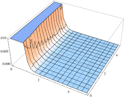
Figure 1: Graph of energy density for $G_{2}+G_{3}$.

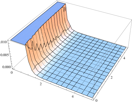
Figure 2: Graph of pressure for $G_{2}+G_{3}$.

7 Conclusion

A variety of new exact solutions of the governing equation (3d), using the Lie method of infinitesimal generators, have been obtained. Previously known solutions where shown to be characterized by a particular Lie generator and are contained, as a special case, in our new family of solutions. We considered each element in the optimal system of one-dimensional subgroups and reduced the master equation to an ordinary differential equation. We were in a position to solve the resulting equations and obtain several new solutions for the gravitating model. A pleasing feature of our analysis is that several models generated admit a linear barotropic equation of state. The pivotal equation has six Lie point symmetries with eight nonzero Lie bracket relationships which generates the optimal system. It is this geometric structure which has enabled us to show that equation (3d) has a rich structure.

Acknowledgements
AMM and KSG thank the National Research Foundation and the University of KwaZulu-Natal for financial support. SDM acknowledges that this work is based upon research supported by the South African Research Chair Initiative of the Department of Science and Technology and the National Research Foundation. We thank Dr J-C Ndogmo for helpful discussions on the structure of Lie algebras.

References

References

- [1] Bluman G W and Kumei S K 1989 Symmetries and Differential Equations (New York: Springer–Verlag)
- [2] Cheviakov A F 2007 Comp. Phys. Comm. 176 48
- [3] Dahia F and Romero C 2002a J. Math. Phys. 43 3097
- [4] Dahia F and Romero C 2002b J. Math. Phys. 43 5804
- [5] Dahia F, Romero C and Guz M A S 2008 J. Math. Phys. 49 112501
- [6] Dimas S and Tsoubelis D 2005 SYM: A new symmetry-finding package for Mathematica Proceedings of The 10th International Conference in Modern Group Analysis ed Ibragimov N H, Sophocleous C and Pantelis P A (Larnaca: University of Cyprus) 64-70
- [7] Gupta Y K and Sharma J R 1996 Gen. Relativ. Gravit. 28 1447
- [8] Head A K 1993 Comp. Phys. Comm. 77 241
- [9] Hereman W 1994 Euromath. Bull. 1 45
- [10] Komathiraj K and Maharaj S D 2007 Int. J. Mod. Phys. D 16 1803
- [11] Krasinski A 1997 Inhomogeneous Cosmological models (Cambridge: Cambridge University Press)
- [12] Lobo F S N 2006 Class. Quantum Grav. 23 1525
- [13] Mak M K and Harko T 2004 Int. J. Mod. Phys. D 13 149
- [14] Olver P J 1993 Applications of Lie Groups to Differential Equations (New York: Springer-Verlag)
- [15] Rand D, Winternitz P and Zassenhaus H 1988 Linear Algebra Appl. 109 197
- [16] Sharma R and Maharaj S D 2007 Mon. Not. R. Astron. Soc. 375 1265
- [17] Stephani H, Kramer D, MacCallum M A H, Hoenselaers C and Herlt E 2003 Exact solutions to Einstein’s field equations (Cambridge: Cambridge University Press)
- [18] Stephani H 1967b Commun. Math. Phys. 5 337
- [19] Stephani H 1967b Commun. Math. Phys. 4 137
- [20] Thirukkanesh S and Maharaj S D 2008 Class. Quantum Grav. 25 235001
- [21] Turkowski P 1990 J. Math. Phys. 31 1344
- [22] Witten E 1984 Phys. Rev. D 30 272
- [23] Wolfram S 1999 The Mathematica Book (Champaign: Wolfram Media)