Polarization correlations in the two–photon decay of hydrogen–like ions

Abstract

Polarization properties of the photons emitted in the two–photon decay of hydrogen–like ions are studied within the framework of the density matrix and second-order perturbation theory. In particular, we derive the polarization correlation function that gives the probability of the (two–photon) coincidence measurement performed by polarization–sensitive detectors. Detailed calculations of this function are performed for the $2s_{1/2}\to 1s_{1/2}$ transition in neutral hydrogen as well as Xe⁵³⁺ and U⁹¹⁺ ions. The obtained results allow us to understand the influence of relativistic and non–dipole effects on the polarization correlations in the bound–bound two–photon transitions in heavy ions.

1 Introduction

Studies on the two–photon decay of atomic hydrogen and hydrogen–like ions have by now a long tradition both in theory and experiment SaP98 ; IlU06 . Originally focused on the total transition rates, the interest in these studies has been recently shifted towards the energy and angular distributions as well as the polarization properties of the emitted photons. A series of $\gamma$–$\gamma$ coincidence experiments were performed, for example, to measure the polarization correlations in the $2s_{1/2}\to 1s_{1/2}$ decay of low–$Z$ ions. When compared with theoretical predictions, the experimental results provided an accurate test of Bell s inequality and hidden variable theories PeD85 ; KlD97 . In contrast to low–$Z$ systems, much less attention has been paid to the polarization properties of the photons emitted in the decay of heavy ions. Only in the light of recent improvements in x–ray detector techniques TaS06 , the observation of $\gamma$–$\gamma$ (polarization) correlations in high–$Z$ domain becomes more likely within the next few years. Beside the detailed analysis of relativistic and quantum electrodynamics (QED) effects, these future coincidence experiments might provide an alternative and very promising route for studying the parity–violation phenomena in heavy atomic systems or even for testing the symmetry violations of Bose particles FrS10 .

In this contribution, we apply the density matrix approach in order to analyze the spin properties of the photons emitted in the (two–photon) decay of hydrogen–like ions. We pay special attention to the so–called polarization correlation function that reflects the probability of the $\gamma$–$\gamma$ coincidence measurement performed by two polarization–sensitive detectors. The basic relations for such a “polarization–polarization coincidence” scenario are given in Sections 2 and 3. In those sections, we discuss how the polarization correlation function can be expressed in terms of second–order transition amplitude. Even though the evaluation of these amplitudes is a rather complicated task due to the summation over the complete spectrum of the system, it can be significantly simplified within the non–relativistic dipole approximation for the electron–photon interaction. Making use of such approximation, we are able then to derive a simple analytical expression for the correlation function. In Section 4 we employ this expression together with the results from our exact relativistic calculations in order to investigate polarization correlations in the $2s_{1/2}\to 1s_{1/2}$ decay of neutral hydrogen as well as Xe⁵³⁺ and U⁹¹⁺ ions. Results of our calculations demonstrate that relativistic and non–dipole contributions may significantly modify the polarization correlation function and that the effect becomes most pronounced for unequal energy sharing between the two photons. A brief summary of our results is given finally in Section 5.

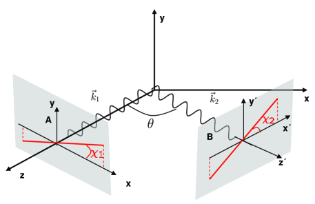
Figure 1: Geometry for the two–photon decay of excited ionic state.

2 Geometry and labeling

In order to investigate the polarization correlations in the two–photon decay of hydrogen–like ions, we shall first agree about the geometry under which the emission of both photons is considered. Since, for the decay of unpolarized ionic states, there is no direction initially preferred for the overall system, we adopted the $z$ axis along the momentum of the “first” photon. Together with the momentum direction of the “second” photon, this axis then defines also the reaction plane (x -z plane). A single polar angle $\theta$, the so–called opening angle, is required, therefore, to characterize the emission of the photons with respect to each other (cf. Fig. 1).

As required by Bose–Einstein statistics, the two–photon state has to be symmetric upon exchange of the particles. Therefore, it is a priori not possible to address them individually. We can safely assume, however, an experimental setup in which two detectors observe (in coincidence) the photons having certain energies and propagation directions. A “click” at these detectors would correspond to the photon’s collapse into energy and momentum eigenstates TiM09 ; FrT10 . A clear identity can be given, therefore, to the photons: the first (second) photon is that one detected by the detector $A(B)$ (marked gray in Fig. 1) at a certain energy $\omega_{1(2)}$ and momentum $\bm{k}_{1(2)}$.

For the theoretical analysis below we shall take into account not only the emission angles and the energies but also the linear polarization states of the emitted photons. In order to observe these states, we assume that both detectors act as linear polarizers whose transmission axes are defined in the planes that are perpendicular to the photon momenta $\bm{k}_{1}$ and $\bm{k}_{2}$ and are characterized by the angles $\chi_{1}$ and $\chi_{2}$ with respect to the reaction (x–z) plane. In this notation, $\chi_{1(2)}=0^{\circ}$ denotes the polarization direction of the first (second) photon within the reaction plane.

3 Theory

Within the framework of the second–order perturbation theory, the analysis of the total as well as differential two–photon decay rates is usually traced back to the evaluation of the transition amplitude DrG81 ; GoD81 :

$$\begin{array}[]{l l l}\displaystyle\mathcal{M}_{fi}^{\bf k_{1}\bf k_{2}}(\lambda_{1},\lambda_{2})&=&\displaystyle{\displaystyle\sum_{\nu}}\!\!\!\!\!\!\!\!\int\left[\frac{\mathinner{\langle{f}|}{\vec{\alpha}}\cdot\bf u_{\lambda_{1}}^{*}e^{-i\bf k_{1}\cdot\bf r}\mathinner{|{\nu}\rangle}\mathinner{\langle{\nu}|}{\vec{\alpha}}\cdot\bf u_{\lambda_{2}}^{*}e^{-i\bf k_{2}\cdot\bf r\,^{\prime}}\mathinner{|{i}\rangle}}{E_{\nu}-E_{i}+\omega_{2}}\right.\\ &&\left.\displaystyle+\frac{\mathinner{\langle{f}|}{\vec{\alpha}}\cdot\bf u_{\lambda_{2}}^{*}e^{-i\bf k_{2}\cdot\bf r}\mathinner{|{\nu}\rangle}\mathinner{\langle{\nu}|}{\vec{\alpha}}\cdot\bf u_{\lambda_{1}}^{*}e^{-i\bf k_{1}\cdot\bf r\,^{\prime}}\mathinner{|{i}\rangle}}{E_{\nu}-E_{i}+\omega_{1}}\right]\,,\end{array}$$ (1)

where $\langle\bm{r}|i\rangle=\psi_{n_{i}j_{i}\mu_{i}}(\bm{r})$ and $\langle\bm{r}|f\rangle=\psi_{n_{f}j_{f}\mu_{f}}(\bm{r})$ are the well–known solutions of the Dirac-Coulomb equation for a single electron in the initial and final states, correspondingly. In this expression, moreover, the transition operator $\vec{\alpha}\,\vec{u}_{\lambda_{j}}\,e^{i\vec{k}_{j}\cdot\vec{r}}$ describes the relativistic electron–photon interaction with $\vec{u}_{\lambda_{j}}$ and $\vec{k}_{j}$ being the polarization and the wave vector of the $j$–th photon.

The evaluation of the amplitude (1) is not a simple task owing to the intermediate–state summation that includes not only the summation over the discrete part of the spectrum but also an integration over the positive as well as the negative–energy continuum. A number of methods have been proposed in the past to carry out such a summation DrG81 . In the present work, the second–order transition amplitude (1) is evaluated by means of the Green’s function approach. Since this approach has been widely applied over the last years for the analysis of the total two–photon decay rates as well as the polarization and angular correlation functions SuR09 ; RaS08 , it will not be recalled here.

After a brief discussion of the second–order transition amplitude (1), we are now ready to analyze the polarization properties of the emitted photons. Most naturally, such an analysis can be performed in the framework of the density matrix theory. For the decay of an unpolarized initial state $\mathinner{|{n_{i}j_{i}}\rangle}$ into the level $\mathinner{|{n_{f}j_{f}}\rangle}$, the two–photon spin density matrix reads as:

$$\displaystyle\mathinner{\langle{\vec{k}_{1},\lambda_{1},\vec{k}_{2},\lambda_{2}}|}\hat{\rho}_{f}\mathinner{|{\vec{k}_{1},\lambda_{1}^{\prime},\vec{k}_{2},\lambda_{2}^{\prime}}\rangle} = \frac{1}{2j_{i}+1}\,\sum_{\mu_{i},\mu_{f}}\mathcal{M}_{fi}^{\vec{k}_{1}\vec{k}_{2}}(\lambda_{1},\lambda_{2})\mathcal{M}_{fi}^{\vec{k}_{1}\vec{k}_{2}\,*}(\lambda_{1}^{\prime},\lambda_{2}^{\prime})\,,$$ (2)

where $\lambda_{j}=\pm 1$ are the spin projections of the photons onto their propagation directions (i.e. the so–called helicity). Instead of this helicity representation, it might be more convenient to re–write the density matrix (2) in the representation of the vectors $\vec{u}_{x}$ and $\vec{u}_{y}$. Such vectors denote the linear polarization of the photons respectively under the angles $\chi=0^{\circ}$ and $\chi=90^{\circ}$ with respect to the reaction plane (see Fig. 1). Any linear polarization which is nowadays measured in experiments can be expressed in terms of these two (basis) vectors

$$\vec{u}_{\chi}=\frac{1}{\sqrt{2}}\,\left(\cos\chi\vec{u}_{x}+\sin\chi\vec{u}_{y}\right)=\frac{1}{\sqrt{2}}\,\left({\rm e}^{-i\chi}\vec{u}_{\lambda=+1}+{\rm e}^{+i\chi}\vec{u}_{\lambda=-1}\right)\,,$$ (3)

by following the standard decomposition of linear polarization vectors in terms of the circular polarization ones.

The density matrix (2) still contains complete information on two photons and, hence, can be employed to derive their polarization properties. To achieve this, it is convenient to define the so–called “detector operator” that projects out all those quantum states of the final–state system which lead to a “count” at the detectors. Since in our present work we wish to analyze the correlated linear polarization states of the photons, the detector operator can be written as:

$$\displaystyle\hat{P} = \mathinner{|{\vec{k}_{1}\chi_{1}\,\vec{k}_{2}\chi_{2}}\rangle}\mathinner{\langle{\vec{k}_{1}\chi_{1}\,\vec{k}_{2}\chi_{2}}|}\,.$$ (4)

From this projector operator, by taking the trace over its product with the density matrix (2) and applying Eq. (3), we immediately derive the polarization–polarization correlation function:

$$\displaystyle\Phi_{\chi_{1},\chi_{2}}(\theta) = \mathcal{N}\,{\rm Tr}(\hat{P}\hat{\rho}_{f})=\frac{\mathcal{N}}{4(2j_{i}+1)}\,\sum\limits\limits_{\lambda_{1}\lambda^{\prime}_{1}\lambda_{2}\lambda^{\prime}_{2}}$$ (5)

$$\times {\rm e}^{i(\lambda_{1}-\lambda^{\prime}_{1})\chi_{1}}\,{\rm e}^{i(\lambda_{2}-\lambda^{\prime}_{2})\chi_{2}}\,\mathcal{M}_{fi}^{\vec{k}_{1}\vec{k}_{2}}(\lambda_{1},\lambda_{2})\mathcal{M}_{fi}^{\vec{k}_{1}\vec{k}_{2}\,*}(\lambda_{1}^{\prime},\lambda_{2}^{\prime})\,,$$

which represents the normalized probability of coincidence measurement of two photons with well–defined wave vectors $\vec{k}_{1}$ and $\vec{k}_{2}$ and with linearly polarization vectors characterized by the angles $\chi_{1}$ and $\chi_{2}$ with respect to reaction plane. Here the normalization constant $\mathcal{N}$ is chosen in such a way that, for any value of the opening angle $\theta$, we get the unity after having summed over the probabilities of the (four) independent photons’ polarization states $\mathinner{|{xx}\rangle}$, $\mathinner{|{xy}\rangle}$, $\mathinner{|{yx}\rangle}$, $\mathinner{|{yy}\rangle}$. For the sake of brevity, we have introduced the notation $\mathinner{|{xx}\rangle}=\mathinner{|{\chi_{1}=0^{\circ}}\rangle}\mathinner{|{\chi_{2}=0^{\circ}}\rangle}$, $\mathinner{|{xy}\rangle}=\mathinner{|{\chi_{1}=0^{\circ}}\rangle}\mathinner{|{\chi_{2}=90^{\circ}}\rangle}$ and so forth.

Any further evaluation of the polarization correlation (5) requires, in general, a computation of the fully–relativistic transition amplitude (1). This amplitude accounts for the full interaction $\vec{\alpha}\,\vec{u}_{\lambda}\,e^{i\vec{k}\cdot\vec{r}}$ between the electron and the radiation field and, hence, includes the higher non–dipole effects. The non–dipole corrections, however, are usually expected to be negligible for low–$Z$ ions. For these ions, it is therefore justified to threat the electron–photon interaction within the non–relativistic dipole approximation by setting $e^{i\vec{k}\cdot\vec{r}}\approx 1$. Within such dipole approximation, a simple analytic expression for the function $\Phi$ can be obtained:

$$\Phi^{2E1}_{\chi_{1},\chi_{2}}(\theta)=\frac{1}{1+\cos^{2}\theta}\Big{(}\sin\chi_{1}\sin\chi_{2}+\cos\chi_{1}\cos\chi_{2}\cos\theta\Big{)}^{2}\,,$$ (6)

for the particular case of the $2s_{1/2}\to 1s_{1/2}$ two–photon transition.

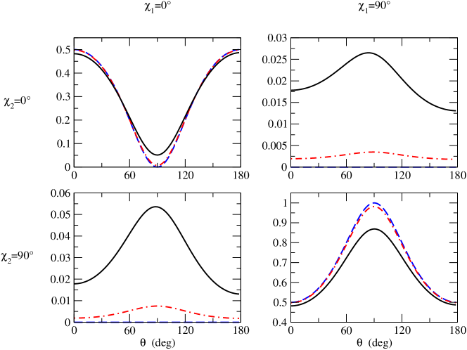
Figure 2: (Color online) Polarization–polarization correlations of photons emitted in the $2s_{1/2}\to 1s_{1/2}$ two–photon decay. The solid line corresponds to U⁹¹⁺, the dot–dashed line corresponds to Xe⁵³⁺ while the dashed line corresponds both to H and to the non–relativistic calculation, since the discrepancy between them less is than $10^{-10}$%. Calculations are presented for the energy sharing $x$ = 1/16 and for the different angles $\chi_{i}$ of the (polarization) transmission axes of detectors (cfr. Fig. 1).

4 Results and discussion

In the present work, we have employed both the non–relativistic electric–dipole approximation (6) and the exact relativistic treatment from Eq. (5) in order to investigate the polarization correlations between the photons emitted in the $2s_{1/2}\to 1s_{1/2}$ decay. For this bound–bound transition, calculations have been performed for neutral hydrogen atom H, hydrogen–like xenon Xe⁵³⁺ and uranium U⁹¹⁺ ions, for various values of the energy sharing parameter. This parameter reflects the fraction of energy carried away by the “first” photon: $x=\omega_{1}/(\omega_{1}+\omega_{2})$ and, hence, is defined in the range $0\leq x\leq 1$. In Fig. 2, for example, the polarization correlation function $\Phi(\theta)$ is displayed for the parameter $x$ = 1/16. As seen from the figure, for light ions, both the electric dipole and the fully relativistic treatments basically coincide and are well described by Eq. (6). In particular, the polarization correlation function $\Phi$ almost vanishes if the polarization axes of detectors are perpendicular to each other: $\chi_{1}$ = 0^∘ and $\chi_{2}$ = 90^∘ or $\chi_{1}$ = 90^∘ and $\chi_{2}$ = 0^∘. Such a behaviour can be understood if we recall that —within the non–relativistic electric dipole approximation— photons are emitted in a pure spin state described by the state vector FrT10 :

$$\mathinner{|{\Psi_{2\gamma}}\rangle}^{2E1}=\frac{1}{1+\cos^{2}\theta}\,\left(\mathinner{|{yy}\rangle}+\cos\theta\mathinner{|{xx}\rangle}\right)\,.$$ (7)

From this expression, it immediately follows that the probability of measuring –in coincidence– orthogonal linear polarizations of photons is zero.

For high–$Z$ hydrogen–like ions, we expect that Eqs. (6)–(7) might not describe well the polarization properties of the emitted photons, owing to relativistic and non–dipole effects. As seen from Fig. 2, these effects result in a non–vanishing correlation function $\Phi$ for the “perpendicular polarization” measurements, i.e. when $\chi_{2}=\chi_{1}\pm 90^{\circ}$. The probability of “parallel polarization” measurements consequently decreases of the same measure. We moreover notice that, in case of energy sharing $x$ = 1/16 and $\theta=90^{\circ}$, events with photon polarizations within the reaction plane are not forbidden, in contrast to the non–relativistic dipole approximation, as a consequence of relativistic and non–dipole effects. This, in turn, leads to a further reduction of the probability for those events with photon polarizations which are perpendicular to the reaction plane. For hydrogen–like uranium ions U⁹¹⁺, for example, the function $\Phi_{\chi_{1},\chi_{2}}$, as calculated at $\chi_{1}=\chi_{2}=90^{\circ}$ and perpendicular photon emission ($\theta=90^{\circ}$), decreases from 1 to almost 0.85 if the higher multipole terms are taken into account.

While the relativistic and retardation effects are significant in high–$Z$ domain if one of the photons is much more energetic than the second one, they become almost negligible if the photons are emitted with nearly the same energy: $\omega_{1}\approx\omega_{2}$. As can be seen from Fig. 3, for energy sharing $x$ = 0.5, the polarization probabilities obtained within non–relativistic electric–dipole and rigorous relativistic approaches differ in fact only of about $\sim 10^{-3}$, even for the decay of hydrogen-like uranium ions.

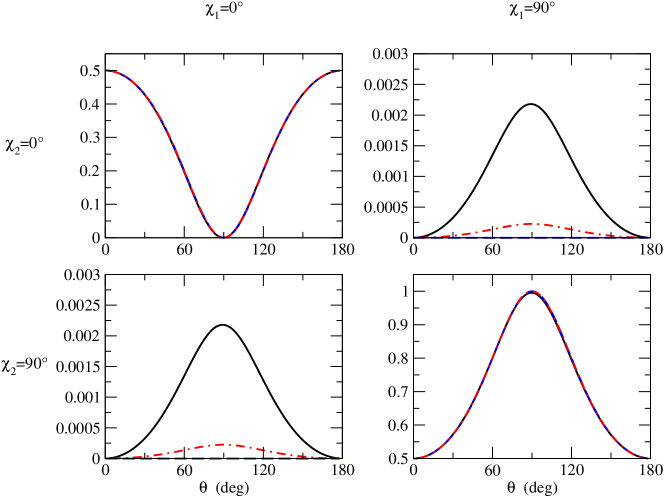
Figure 3: (Color online) Polarization–polarization correlations of photons emitted in the $2s_{1/2}\to 1s_{1/2}$ two–photon decay. The solid line corresponds to U⁹¹⁺, the dot–dashed line corresponds to Xe⁵³⁺ while the dashed line corresponds both to H and to the non–relativistic calculation, since the discrepancy between them less is than $10^{-10}$%. Calculations are presented for the energy sharing $x$ = 1/2 and for the different angles $\chi_{i}$ of the (polarization) transmission axes of detectors (cfr. Fig. 1).

5 Summary and outlook

In summary, the polarization of the radiation emitted in the two-photon decay of hydrogen–like ions has been investigated within the framework of the second–order perturbation theory. Special attention has been paid to the correlated spin states of two photons as can be measured in coincidence $\gamma-\gamma$ experiments. In order to predict the outcome of such experiments, the expression for the polarization correlation function has been derived within both the exact relativistic theory and the non–relativistic electric–dipole approximation. Making use of these two approaches, the photon–photon polarization correlations have been calculated for the $2s_{1/2}\to 1s_{1/2}$ transition in neutral hydrogen as well as hydrogen–like Xe⁵³⁺ and U⁹¹⁺ ions. As seen from the results obtained, the higher non–dipole terms in the electron–photon interaction may affect the correlation function by about 10–20 %; effect that becomes most pronounced for the decay of high–$Z$ ions if the major fraction of the (two -photon) transition energy is carried away by a single photon.

In the present work, we have restricted our theoretical analysis of the two–photon decay to the one–electron atomic systems. For high–$Z$ domain, however, the helium–like ions are the most suitable candidates for two–photon studies. In the future, therefore, we plan to extend our theoretical approach for studying transitions in these two–electron species. A first case study on the polarization correlations and spin entanglement in the $1s_{1/2}2s_{1/2}:J=0\to 1s_{1/2}^{2}:J=0$ decay of U⁹⁰⁺ ions is currently under way and will be published soon.

- (1) J. P. Santos, F. Parente, and P. Indelicato, Eur. Phys. J. D 3, 43 (1998), and references therein.
- (2) K. Ilakovac, M. Uroić, M. Majer, S. Pasić, and B. Vuković, Radiat. Phys. Chem. 75, 1451 (2006), and references therein.
- (3) W. Perrie, A. J. Duncan, H. J. Beyer, and H. Kleinpoppen, Phys. Rev. Lett. 54, 1790 (1985).
- (4) H. Kleinpoppen, A. J. Duncan, H. J. Beyer, and Z. A. Sheikh, Phys. Scr., T72, 7 (1997).
- (5) S. Tashenov, Th. Stölker, D. Banas, K. Beckert, P. Beller, H.F. Beyer, F. Bosch, S. Fritzsche, A. Gumberidze, S. Hangmann, C. Kozhuharov, T. Krings, D. Liesen, F. Nolden, D. Protic, D. Sierpowski, U. Spillmann, M. Steckm, A. Surzhykov, Phys. Rev. Lett., 97, 223202 (2006).
- (6) F. Fratini and A. Surzhykov, to be published.
- (7) M. C. Tichy, F. de Melo, M. Kuś, F. Mintert, and A. Buchleitner, arXiv:0902.1684 (2009)
- (8) F. Fratini, M.C. Tichy, T. Jahrsetz, S. Fritzsche and A. Surzhykov, to be published.
- (9) G. W. F. Drake and S. P. Goldman, Phys. Rev. A, 23, 2093 (1981).
- (10) S. P. Goldman and G. W. F. Drake, Phys. Rev. A, 24, 183 (1981).
- (11) A. Surzhykov, T. Radtke, P. Indelicato and S. Fritzsche, Eur. Phys. J. Special Topics, 169, 29 (2009).
- (12) T. Radtke, A. Surzhykov, and S. Fritzsche, Phys. Rev. A, 77, 0022507 (2008).
- (13) R.A. Swainson and G.W. Drake, J.Phys.A: Math. Gen., 24, 95 (1991)
- (14) M. E. Rose, Elementary theory of angular momentum, John Wiley & Sons (1963).