On the growth and orbital evolution of giant planets in layered protoplanetary disks

Abstract

Aims. We present the results of hydrodynamic simulations of the growth and orbital evolution of giant planets embedded in a protoplanetary disk with a dead-zone. The aim is to examine to what extent the presence of a dead-zone affects the rates of mass accretion and migration for giant planets.

Methods. We performed 3D numerical simulations using a grid–based hydrodynamics code. In these simulations of laminar, non-magnetised disks, the dead-zone is treated as a region where the vertical profile of the viscosity depends on the distance from the equatorial plane. We consider dead-zones with vertical sizes, $H_{DZ}$, ranging from $0$ to $H_{DZ}=2.3H$, where $H$ is the disk scale-height. For all models, the vertically integrated viscous stress, and the related mass flux through the disk, have the same value (equivalent to $10^{-8}$ M_⊙yr^-1), such that the simulations test the dependence of planetary mass accretion and migration on the vertical distribution of the viscous stress (and mass flux). For each model, an embedded $30\;M_{\oplus}$ planet on a fixed circular orbit is allowed to accrete gas from the disk. Once the planet mass becomes equal to that of Saturn or Jupiter, we allow the planet orbit to evolve due to gravitational interaction with the disk.

Results. We find that the time scale over which a protoplanet grows to become a giant planet is essentially independent of the dead-zone size, and depends only on the total rate at which the disk viscously supplies material to the planet. For Saturn-mass planets, the migration rate depends only weakly on the size of the dead-zone for $H_{DZ}\leq 1.5H$, but becomes noticeably slower when $H_{DZ}=2.3H$. This effect is apparently due to the desaturation of corotation torques which originate from residual material in the partial-gap region. For Jupiter-mass planets, there is a clear tendency for the migration to proceed more slowly as the size of the dead-zone increases, with migration rates differing by approximately 40 % for models with $H_{DZ}=0$ and $H_{DZ}=2.3H$.

Conclusions. Our results indicate that for disks models in which the mass accretion rate has a well defined value, the accretion and migration rates for Saturn- and Jovian-mass planets are relatively insensitive to the presence and size of a dead-zone.

1 Introduction

Multiple observations of star-forming regions have revealed that young stars are surrounded by circumstellar disks composed of gas and dust (e.g. Beckwith 1996, Sicilia-Aguilar et al. 2006), which are thought to provide the necessary material for planet formation. These protoplanetary disks generally show evidence for gas accretion onto the central star, with a typical mass flow being $\sim 10^{-8}$ M_⊕ yr^-1 (Sicilia-Aguilar et al. 2004; Gullbring et al. 1998; Haisch et al. 2001). It has long been recognized that such a value for the accretion rate requires a source of anomalous viscosity, probably originating from turbulence, to efficiently transport the angular momentum outward (Shakura & Sunyaev 1973).
Although instabilities such as the baroclinic instability (Klahr & Bodenheimer 2003) or the Rossby-wave instability (Lovelace et al. 1999) may result in turbulence, a significant number of studies (Hawley et al. 1996; Brandenburg et al. 1996) have shown that the non-linear outcome of the magnetorotational instability (Balbus & Hawley 1991; hereafter MRI) is MHD turbulence with an effective viscous stress parameter $\alpha\sim 5\times 10^{-3}$, providing the necessary angular momentum transport to match the observed accretion rates onto T-Tauri stars (Hartmann et al. 1998).
Although the MRI has been proven robust in generating MHD turbulence, the fact that the ionisation fraction is expected to be low in protoplanetary disks (Blaes & Balbus 1994) raises a number of question about the applicability of the MRI in these environments. That is the reason why it has been suggested (Gammie 1996) that protoplanetary disks may have both magnetically active zones near the surface, where cosmic ray ionisation enables the MRI to develop, and a “dead-zone” close to the disk midplane where the flow remains laminar. This layered-disk picture was confirmed by Fleming & Stone (2003) who performed MHD simulations of stratified disks in which the magnetic resistivity decreases as a function of height. Over the past few years, many studies have focused on the structure of the dead-zone by using different chemical reaction networks. Fromang et al. (2002) showed that the size of the dead-zone can decrease in the presence of heavy metals (such as magnesium) due to charge-transfer reactions. Ilgner & Nelson (2006b) examined the role of turbulent mixing, and showed that in the presence of magnesium, such a process can enliven the dead-zone beyond a few AU. This was confirmed by Ilgner & Nelson (2008) who performed multifluid MHD simulations and who showed that despite the addition of gas-phase magnesium, dead-zones in protoplanetary disks typically persist at distances $R\leq 5$ AU, with potentially important consequences for planet formation in these regions. Calculations which examine the sizes of dead-zones including gas-grain chemistry, show that the presence of a modest population of sub-micron sized grains cause the planet forming regions of protoplanetary disks to host significant dead-zones (Sano et al. 2000; Ilgner & Nelson 2006a; Turner & Drake 2009).
So far, the effect of a dead-zone on planet formation has received little attention, in large part because of the computational expense of performing large-scale 3D MHD simulations of turbulent protoplanetary disks. A plausible scenario for the formation of planets involves the following steps: i) coagulation and settling of dust in the disk midplane, followed by the growth of km-sized planetesimals; ii) runaway growth of planetesimals (e.g. Greenberg et al. 1978; Wetherill & Stewart 1989) into $\sim 10^{-5}\;M_{\oplus}$ embryos; iii) oligarchic growth of these embryos (e.g. Kokubo & Ida 1998, 2000; Leinhardt & Richardson 2005) into planetary cores. Planetary cores forming oligarchically beyond the snow-line are expected to have masses $\sim 10\;M_{\oplus}$ (Thommes et al. 2003) and consequently are able to accrete a gaseous envelope to become giant planets (Pollack et al. 1996).

The impact of a dead-zone on dust settling was examined by Fromang & Papaloizou (2006) who found a tendency for thinner dust sub-disks to form in the presence of a dead-zone. Lyra & al. (2008, 2009) found that a Rossby-wave instability can be triggered at the border of a dead-zone where the surface density is significantly enhanced, creating vortices which are efficient in trapping solids and forming planetary embryos.
The consequence of a dead-zone on planet migration was studied by Matsumura et al. (2003). These authors found that a dead-zone significantly slows down the migration of low-mass planets undergoing Type I migration. This arises because the dead-zone creates a jump in surface density, which changed the balance between inner and outer Lindblad torques in their model. A surface density transition, however, can also create a planet trap where the corotation torque exerted on the protoplanet equals the differential Lindblad torque (Masset et al. 2006). Concerning gap-opening giant planets which migrate on a viscous timescale, Matsumura et al. (2003) found, unsurprisingly, that a dead-zone slows down Type II migration due to the low value for the viscosity there. However, it should be noted that this work did not consider how the existence of a live-zone near the disk surface affects this latter result.
In this paper, we present the results of 3D hydrodynamical simulations of giant-planets embedded in layered protoplanetary disks and in which the dead-zone is modelled using a vertical profile for the laminar viscosity which increases as a function of height in the disk. The aim of this work is to investigate how the evolution depends on the size of the dead-zone $H_{DZ}$, subject to the condition that all our disk models have the same vertically integrated viscous stress and associated radial mass flux. To address this issue, we consider a model in which a $30\;M_{\oplus}$ protoplanet is embedded in the disk on a fixed circular orbit, and can slowly accrete gas until its mass $m_{p}$ becomes the same as that of Saturn ($m_{p}=1$ M_S) or Jupiter ($m_{p}=1$ M_J). The planet is then released and allowed to evolve under the action of disk forces. The results of these simulations suggest that for a given accretion rate through the disk, Jupiter migrates more slowly as the size of the dead-zone increases. However, we find that provided the size of the dead-zone is small enough, both the accretion rate onto the planet and the migration of Saturn-mass planets depend only weakly on $H_{DZ}$.

This paper is organized as follows. In Sect. 2, we describe the hydrodynamical model and the numerical setup. In Sect. 3, we present the results of our simulations. We finally summarize and draw our conclusions in Sect. 4.

2 Physical model and numerical setup

In order to study the evolution of a giant planet in a dead-zone, which is represented in the simulations as a disk region where the viscosity profile depends on the distance from the equatorial plane, we adopt a 3-dimensional disk model. In spherical coordinates $(r,\theta,\phi)$ and in a frame centred on the central star, the continuity equation reads:

$$\frac{\partial\rho}{\partial t}+\nabla\cdot(\rho{\bf v})=0$$ (1)

where $\rho$ is the disk density. The equations for the radial, meridional, and angular components of the disk velocity ${\bf v}=(v_{r},v_{\theta},v_{\phi})$ are given, respectively, by:

$$\frac{\partial(\rho v_{r})}{\partial t}+\nabla\cdot(\rho v_{r}{\bf v})=\frac{\rho(v_{\theta}^{2}+v_{\phi}^{2})}{r}-\frac{\partial p}{\partial r}-\rho\frac{\partial\Phi}{\partial r}+f_{r},$$ (2)

$$\frac{\partial(\rho v_{\theta})}{\partial t}+\nabla\cdot(\rho v_{\theta}{\bf v})=-\frac{\rho v_{r}v_{\theta}}{r}-\frac{\rho v_{\phi}^{2}\cot\theta}{r}-\frac{1}{r}\frac{\partial p}{\partial r}-\frac{\rho}{r}\frac{\partial\Phi}{\partial r}+f_{\theta}$$ (3)

and

$$\frac{\partial(\rho v_{\phi})}{\partial t}+\nabla\cdot(\rho v_{\phi}{\bf v})= -\frac{\rho v_{r}v_{\phi}}{r}-\frac{\rho v_{\theta}v_{\phi}\cot\theta}{r}$$ (4)

$$-\frac{1}{r\sin\theta}\frac{\partial p}{\partial r}-\frac{\rho}{r\sin\theta}\frac{\partial\Phi}{\partial r}+f_{\phi}.$$ (5)

In the above equations, $p$ is the pressure, $f_{r}$, $f_{\theta}$ and $f_{\phi}$ are respectively the radial, meridional and azimuthal components of the viscous force per unit volume. Expressions for $f_{r}$, $f_{\theta}$ and $f_{\phi}$ can be found for example in Klahr et al.(1999). $\Phi$ is the gravitational potential and can be written as:

$$\Phi=-\frac{GM_{\star}}{r}-\frac{Gm_{p}}{\sqrt{|{\bf r}-{\bf r_{p}}|^{2}+\epsilon^{2}}}+\Phi_{ind},$$ (6)

where $M_{\star}$ and $m_{p}$ are the masses of the star and planet, respectively, and where $\epsilon$ is a softening length. $\Phi_{ind}$ is an indirect term arising from the fact that the star-centered frame is not inertial. This term reads:

$$\Phi_{ind}=\frac{Gm_{p}}{r_{p}^{3}}{\bf r\cdot r_{p}}+G\int_{V}\frac{dm({\bf r^{\prime}})}{r^{\prime 3}}{\bf r\cdot r^{\prime}},$$ (7)

where the integral is performed over the volume of the disk.

2.1 Planet orbital evolution

In this work the planet can experience the gravitational acceleration arising from both the disk and the central star. Therefore, the equation of motion for the planet is given by:

$$\frac{d^{2}{\bf r_{p}}}{dt^{2}}=-\frac{GM_{\star}}{r_{p}^{3}}{\bf r_{p}}+{\bf f_{dp}}-\nabla\Phi_{ind},$$ (8)

where ${\bf f_{dp}}$ is the force due to the disk which is defined by:

$${\bf f_{dp}}=-G\int_{V}\frac{\rho(\bf{r})({\bf r_{p}}-{\bf r})}{(|{\bf r}-{\bf r_{p}}|^{2}+\epsilon^{2})^{3/2}}dV$$ (9)

Note that we exclude the material contained in the planet Hill sphere when calculating the gravitational force acting on the planet. Moreover, in the simulations presented here, the smoothing length $\epsilon$ is set to the diagonal length of one grid cell.

3 Numerical setup

3.1 Numerical method

The 3D hydrodynamical simulations presented in this paper have been performed using the NIRVANA code (Ziegler & Yorke 1997), which is basically a grid-based code which computes spatial derivatives using finite differences. The advection scheme is based on the monotonic transport algorithm and since it employs a staggered mesh, the numerical method used in this code is spatially second-order accurate. Further details about NIRVANA can be found for example in De Val-Borro et al. (2006).
We adopt computational units in which the mass of the central star is $M_{\star}=1$, the gravitational constant is $G=1$ and the cylindrical radius $R=1$ corresponds to the initial orbital radius of the planet $a_{0}$. In the following, we report our results in units of the initial orbital period of the planet $P=2\pi\Omega_{0}^{-1}$, where $\Omega_{0}=\sqrt{GM_{\star}/a_{0}^{3}}$.
For most of the calculations, we employ $N_{r}=128$ radial grid cells uniformly distributed between $r_{in}=0.4$ to $r_{out}=2.5$, $N_{\phi}=384$ grid cells in azimuth and $N_{\theta}=64$ meridional grid cells with $\theta$ lying in the range $80^{\circ}$ to $90^{\circ}$. Some low resolution runs using $N_{r}=64$, $N_{\phi}=192$ and $N_{\theta}=64$ grid cells have also been performed. These are long-term simulations, aimed at giving the embedded giant planet sufficient time to create a gap in the disk.

3.2 Initial conditions

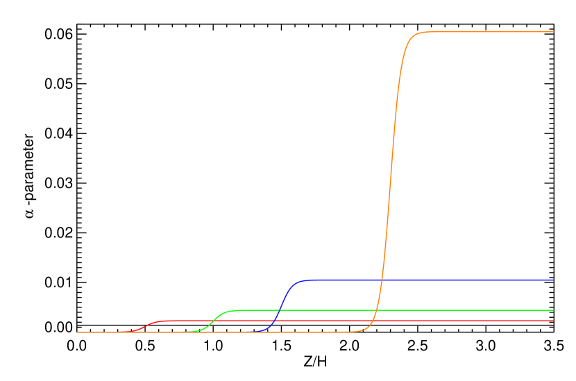
Figure 1: This figure shows the $\alpha$-parameter as a function of the distance from the equatorial plane for the different sizes of the dead-zone we considered, namely for $H_{DZ}/H=0$ (black line), $H_{DZ}/H=0.5$ (red line), $H_{DZ}/H=1$ (green line), $H_{DZ}/H=1.5$ (blue line) and $H_{DZ}/H=2.3$ (orange line).

In the disk model that we adopt for the simulations presented here, the aspect ratio is constant and set to $h=H/R=0.05$, which is a typical value for protoplanetary disks. The initial density profile is chosen such that the vertical stratification of the disk follows the condition for hydrostatic equilibrium and is defined by:

$$\rho=\rho_{0}\left(\frac{R_{0}}{R}\right)^{3/2}\exp\left(-\frac{Z^{2}}{2H^{2}}\right)$$ (10)

where $R$ is the cylindrical disk radius, $Z$ is the distance from the midplane and where $\rho_{0}$ and $R_{0}$ are constants. Consequently, the disk surface density $\Sigma=\int\rho dz$ can be written as $\Sigma=\Sigma_{0}(R_{0}/R)^{-1/2}$, with $\Sigma_{0}=\sqrt{2\pi}hR_{0}\rho_{0}$. Here, we set $R_{0}=1$ and $\rho_{0}$ is chosen such that the disk contains $\sim 3\times 10^{-3}M_{\odot}$ within the computational domain, which corresponds to $\sim 0.02\;M_{\odot}$ interior to 40 AU.
The anomalous viscous stress arising from MHD turbulence is parameterized using the standard ’alpha’ prescription for the disk viscosity $\nu=\alpha c_{s}H$ (Shakura & Sunyaev 1973), where $c_{s}$ is the local speed of sound . From the results of previous MHD simulations (Papaloizou & Nelson 2003; Fromang & Nelson 2006), such a prescription is expected to provide a reasonable description of the mean flow in the disk. It is now understood that low mass planets are subject to stochastic forcing when embedded in turbulent disks (e.g. Nelson & Papaloizou 2004; Nelson 2005), and so the adoption of an anomalous viscous stress to model the effects of turbulence may seem inappropriate at first sight. But, in this work, we are mainly interested in the migration and growth of more massive, gap forming planets where the primary role of turbulence is to supply gas to the vicinity of the planet through an accretion flow generated by the turbulent stresses, and the local interaction between the planet and turbulent density fluctuations is less important (e.g. Nelson & Papaloizou 2003; Papaloizou, Nelson & Snellgrove 2004).

Although it remains to be proven that for a disk with a dead-zone, the stresses arising from MHD turbulence behave like a locally varying laminar viscosity, $\alpha$ is chosen here to be Z-dependent and such that it can vary from very small values in the disk midplane to much higher values near the disk surface. More precisely, in the calculations we performed, the vertical profile adopted for $\alpha$ was as follows:

$$\alpha(Z)=\frac{1}{2}\left\{(\alpha_{AZ}-\alpha_{DZ})\tanh\left(\frac{Z-H_{DZ}}{\Delta}\right)+\alpha_{AZ}+\alpha_{DZ}\right\},$$ (11)

where $H_{DZ}$ is the size of the dead-zone and where $\alpha_{AZ}$ (resp. $\alpha_{DZ}$) is the value for the $\alpha$-parameter in the active (resp. dead) region. In the previous equation, $\Delta$ denotes the size of the transition from the dead to the active zone and is set to $\Delta=0.08H$ in the work presented here. In order to study the influence of the dead-zone size on the evolution of giant planets, we have considered different values for $H_{DZ}$ lying in the range $0$ to $2.3\;H$. In the case where $H_{DZ}=0$, $\alpha$ is constant in the entire disk and is set to $\alpha_{0}=1.4\times 10^{-3}$, which corresponds to a constant accretion rate through the disk $\dot{M}_{0}=3\pi\alpha_{0}\Sigma_{0}h^{2}$. For other values of $H_{DZ}$, we adopt a similar value for the vertically averaged mass flow through the layered disk $\dot{M}=3\pi\int\nu(z)\;\rho dz=\dot{M}_{0}$ and we calculate the value for $\alpha_{AZ}$ accordingly, assuming that the residual viscosity in the dead-zone is $\alpha_{DZ}=1.0\times 10^{-7}$. For the different values of $H_{DZ}$ we considered, the corresponding value for $\alpha_{AZ}$ can be found in Table 1 and Fig. 1 displays the corresponding $\alpha$-parameter as a function of the distance from the disk equatorial plane .

The planet is initially placed on a circular orbit at $a=1$, and our main interest is to examine the orbital evolution of planets with masses $m_{p}=3\times 10^{-4}$ and $10^{-3}\;M_{*}$, corresponding to Saturn-mass ($M_{S}$) and Jupiter-mass ($M_{J}$) planets, respectively. In order to conserve mass as the planet grows and opens a gap, we proceed in two steps:
i) we consider a $30\;M_{\oplus}$ protoplanet held at $a=1$ on a fixed circular orbit. This body is allowed to accrete gas from the disk on a timescale corresponding to $\sim 1500$ orbits. Due to the very long run times required for the planet mass to reach $1\;M_{J}$, we have performed, for this step, low-resolution simulations using $N_{r}=64$, $N_{\phi}=192$ and $N_{\theta}=64$ grid cells.
ii) once the planet mass has reached $1\;M_{S}$ or $1\;M_{J}$, we restart the calculations, but with the planet being allowed to migrate due to its interaction with the disk, and accretion being switched off. For this second step, we have performed higher resolution simulations using $N_{r}=128$, $N_{\phi}=384$ and $N_{\theta}=64$ grid cells. The new values for the disk physical quantities were computed from the old ones using bi-linear interpolation.

Table 1: Dead-zone parameters for the different models considered.

$H_{DZ}/H$	$\alpha_{AZ}$	$\alpha_{DZ}$
$0.5$	$2.3\times 10^{-3}$	$1\times 10^{-7}$
$1$	$4.4\times 10^{-3}$	$1\times 10^{-7}$
$1.5$	$1.05\times 10^{-2}$	$1\times 10^{-7}$
$2.3$	$6.5\times 10^{-2}$	$1\times 10^{-7}$

3.3 Boundary conditions

At the inner edge of the computational domain, we model accretion onto the central star by using a ‘viscous’ boundary condition, for which we set the radial velocity in the innermost cells to $v_{r}=\beta v_{visc}(r_{in})$, where $v_{visc}(r_{in})=-3\nu/2r_{in}$ is the typical disk inward drift velocity due to viscous diffusion, and $\beta$ is a free parameter which is set to $\beta=5$ in this work (Pierens & Nelson 2008). At the outer edge of the computational domain, and at the lower meridional boundary as well, we prevent mass loss from the disk by employing reflecting boundary conditions. Assuming that the disk is symmetric with respect to its midplane, we also impose a symmetry boundary condition at the upper meridional boundary, which corresponds to the disk midplane. Consequently, we consider only the upper half of the disk in the simulations described below.

4 Results

4.1 Effect of the presence of a dead-zone on planetary growth

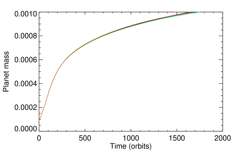
Figure 2: This figure shows the evolution of the planet mass as a function of time for the different sizes of the dead-zone we consider, namely for $H_{DZ}/H=0$ (black line), $H_{DZ}/H=0.5$ (red line), $H_{DZ}/H=1$ (green line), $H_{DZ}/H=1.5$ (blue line) and $H_{DZ}/H=2.3$ (orange line).

For each value of $H_{DZ}$ we consider, we have performed a simulation in which a $30\;M_{\oplus}$ planet held on a circular orbit can accrete gas from the disk until its mass reaches $1\;M_{J}$ . In the simulations presented here accretion is modelled by removing at each time-step a fraction of the gas located inside the Roche lobe of the planet and then adding the corresponding amount of matter to the mass of the planet (e.g. Kley 1999; Nelson et al. 2000). The e-folding time for gas accretion was chosen to be the orbital period of the planet, which corresponds to the maximum rate at which the planet can accrete gas (Kley 1999). The choice of a $30\;M_{\oplus}$ protoplanet to act as a seed onto which gas can accrete is broadly consistent with evolutionary models of gas giant planets forming in protoplanetary disks, which suggest that rapid gas accretion occurs once the planet mass reaches $30-40\;M_{\oplus}$ (Papaloizou & Nelson 2005).
The time evolution of the planet mass for each model is displayed in Fig. 2. We see that the evolution of the planet mass depends only weakly on the size of the dead-zone and proceeds similarly in each case. The early evolution involves rapid gas accretion with the planet growing to become a Saturn-mass planet in $\sim 100$ orbits. As the planet mass increases, non-linear effects can tidally truncate the disk, leading to a decrease in the accretion rate such that it takes $\sim 1500$ orbits for a Saturn-mass planet to reach a Jovian mass.

It is worth noting, however, that although at earlier times the accretion rate should not depend strongly on the size of the dead-zone, since the planet is able to accrete material which is on neighbouring orbits, we expect this to be not true from the time the gravitational torque is largely deposited in the disk in the near-vicinity of the planet. This occurs when the thermal criterion for gap opening is satisfied (Lin & Papaloizou 1986; Crida et al. 2006), namely when the radius of the Hill sphere exceeds the disk semi-thickness:

$$a\left(\frac{m_{p}}{3M_{*}}\right)^{1/3}>H.$$ (12)

In the simulations presented here, this happens roughly when $m_{p}\geq 3\times 10^{-4}$. From this time, the planet may be able to open a gap in the disk provided that the gravitational torques overwhelm the viscous forces (Bryden et al. 1999; Papaloizou et al. 2006), a condition which can be expressed as:

$$\frac{m_{p}}{M_{*}}>\frac{40\nu}{a^{2}\Omega_{p}},$$ (13)

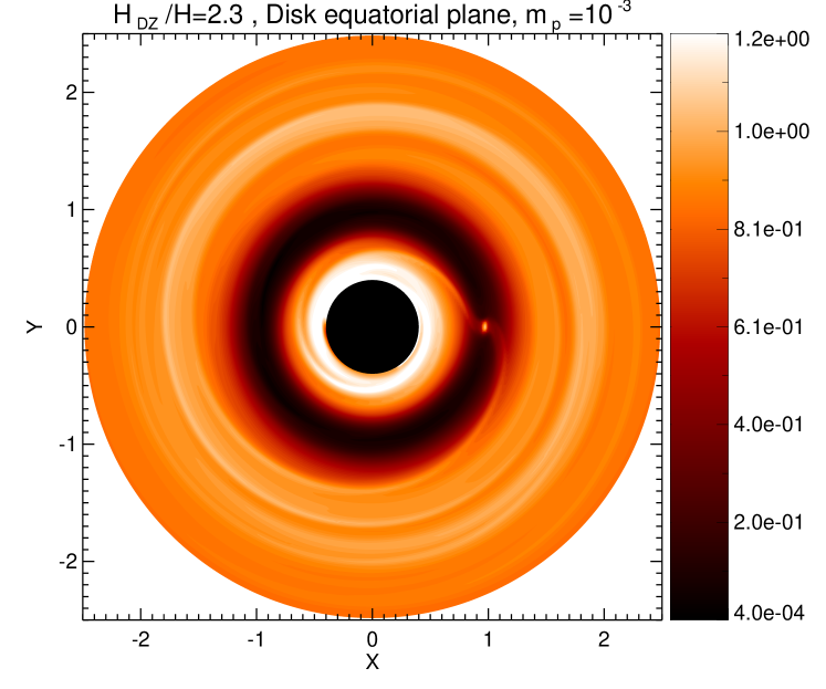
Figure 3: Left panel: this figure shows a snapshot of the disk density in the equatorial plane for $H_{DZ}/H=2.3$. Here, a planet held on a circular orbit at $a=1$ and with initial mass $m_{p}=30\;M_{\oplus}$ has grown to become a Jupiter-mass planet. Right panel: same but at the disk upper surface.

where $\Omega_{p}$ is the angular velocity of the planet. Since the value for the viscosity in the active region is correlated with the size of the dead-zone, the previous equation shows that the gap structure and consequently the accretion rate onto the planet may depend strongly on $H_{DZ}$ for $m_{p}\geq 3\times 10^{-4}$. Indeed, considering for instance the case $m_{p}=1\;M_{J}$, Eq. 13 predicts that gap opening should occur for $\alpha\leq 0.01$. Therefore, in the cases where $H_{DZ}/H=1.5$ and $H_{DZ}/H=2.3$, we expect a $1\;M_{J}$ planet to be able to open a gap only in the dead-zone, possibly leaving the gas flowing over the top of the planet in the active region if the accretion flow there is rapid enough. Snapshots of the disk density in the equatorial plane, and at the disk surface, are depicted in Fig. 3. These plots correspond to a time when the mass of the accreting protoplanet has reached $1\;M_{J}$ and are for a model in which $H_{DZ}=2.3H$. These reveal that the planet truncates the disk throughout its vertical extent, despite the high value for the viscosity in the active region. As can be seen in Fig. 4, such a process arises because the planet is able to pull some of the gas from the live-zone down in toward the midplane as the latter tries to flow over the top of the planet. This suggests that both the gap structure and the accretion rate onto the planet do not depend strongly on the presence of a dead-zone, but rather on the vertically-integrated accretion rate of gas through the disk. In that case, we would expect the results from these 3D runs to not significantly differ from 2D calculations for a given value of the accretion rate $\dot{M}$.

To investigate this issue in more detail, we have performed a suite of 2D runs with varying values of $\alpha$ from $\alpha=0$ to $\alpha=1.4\times 10^{-3}$ and for which the initial surface density at the planet position is $\Sigma(R_{0})=\Sigma_{0}$. An additional 2D calculation with $\alpha=2.8\times 10^{-3}$ and $\Sigma(R_{0})=0.5\Sigma_{0}$ has also been performed. The results of these calculations are shown in Fig. 5. Also displayed are the results of two 3D simulations corresponding to: i) a fully active disk with $\alpha=1.4\times 10^{-3}$ throughout; ii) a dead disk with $\alpha=0$ everywhere. As expected, 2D runs with $\alpha\neq 0$ predict that the protoplanet grows faster as the viscosity increases. The run with $\alpha=2.8\times 10^{-3}$ shows slower growth at earlier times since the surface density is smaller in that case. However, once the planet opens a gap in the disk, it is clear that the growth rate becomes similar to that obtained from the run with ${\alpha=1.4\times 10^{-3}}$ and for which the value for the mass accretion rate through the disk is the same. In the case where $\alpha=0$, viscous supply of gas through the disk is inhibited and the planet mass can saturate once the feeding zone is empty of gas, which occurs when $m_{p}\sim 0.5M_{J}$ for the disk parameters used in this work. Clearly, for both $\alpha=0$ and $\alpha=1.4\times 10^{-3}$, there is a good agreement between 2D and 3D calculations. This confirms that the accretion rate onto a gap-opening planet does not depend strongly on the details of the flow in the $(R,z)$ plane, but only on the vertically-averaged accretion rate through the disk.

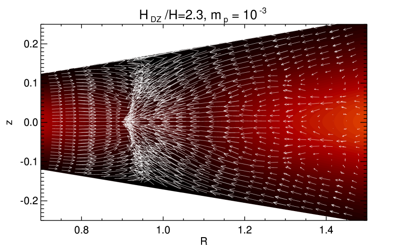
Figure 4: This figure shows, for $H_{DZ}/H=2.3$, details of the flow in the neighbourhood of the accreting planet when its mass has reached $1\;M_{J}$. The velocity field is represented in the $(R,z)$ plane and for ${0.6\leq R\leq 1.5}$.

Figure 5: This figure shows the evolution of the planet mass as a function of time for 2D simulations in which the $\alpha$-parameter was varied from $\alpha=0$ to $\alpha=2.8\times 10^{-3}$. Diamonds display for comparison the results of a 3D run with $H_{DZ}=0$ and $\alpha=1.4\times 10^{-3}$ whereas triangles display the results of a 3D run with $\alpha=0$.

4.2 Effect of a dead-zone on the orbital evolution of Saturn-mass planets

In order to study the evolution of a Saturn-mass planet embedded in a layered protoplanetary disk, we restarted the simulations described in the previous section when the mass of the accreting planet had reached the relevant value. We then released the planet and let it evolve freely under the action of disk torques.
The evolution of Saturn’s semi-major axis for the different models is shown in the upper panel of Fig. 6. For each value of $H_{DZ}/H$, Saturn does not undergo runaway migration (Masset & Papaloizou 2003) because the disk is not massive enough. Instead, the migration rate is intermediate between the Type II and Type I regimes. This arises because the mass of Saturn is insufficient to enable a clean gap to form in the disk, as illustrated in Fig. 8. This figure displays, for the model with $H_{DZ}/H=2.3$, a snapshot of the Saturn-induced gap structure in both the equatorial plane and at the disk surface. It is worthwhile noticing that gap opening occurs in the live-zone, despite the high value for the viscosity there, indicating that both Jupiter and Saturn can pull gas from the active region down toward the disk midplane.
For models with $H_{DZ}/H\leq 1.5$, the evolution of the system proceeds quite similarly, with a slight tendency for the migration rate to decrease as the size of the dead-zone increases. For the calculation with $H_{DZ}/H=2.3$ however, we see that in $\sim 200$ orbits the semi-major axis has decreased by an amount that is nearly $20\%$ less than for the other cases. This can be confirmed by examining the total disk torques exerted on the planet, which are displayed for each model in the lower panel of Fig. 6. It is well known that the total tidal torque, $\Gamma$, exerted on the planet can be written as the sum of a differential Lindblad torque, $\Gamma_{L}$, and a total corotation torque, $\Gamma_{C}$ (Tanaka & Ward 2002). In contrast to $\Gamma_{L}$, which is basically independent of viscosity (Meyer-Vernet & Sicardy 1987; Papaloizou & Lin 1984), $\Gamma_{C}$ depends strongly on $\nu$ and can saturate in the low-viscosity limit. In the present case, $\Gamma_{C}$ can be decomposed as:

$$\Gamma_{C}=\Gamma_{C}^{DZ}+\Gamma_{C}^{AZ},$$ (14)

where $\Gamma_{C}^{DZ}$ (resp. $\Gamma_{C}^{AZ}$) is the corotation torque due to the librating fluid elements which originate from the dead (resp. active) region. In the dead-zone, $\Gamma_{C}^{DZ}$ is expected to saturate on a timescale corresponding to the outermost horseshoe turnover time (Masset 2002)

$$\tau_{HS}=\frac{8\pi a}{3x_{s}}\Omega_{p}^{-1}.$$ (15)

In the previous equation, $x_{s}$ is the horseshoe zone width which can be approximated by $x_{s}=2.45a(q/3)^{1/3}$ (Masset et al. 2006), where $q$ is the planet to central star mass ratio. Here, this gives $\tau_{HS}\sim 71\;\Omega_{p}^{-1}$, which is consistent with the timescale over which the total torques reach a constant value in Fig. 6. In the active region, however, we would expect the corotation torque $\Gamma_{C}^{AZ}$ there to saturate only if the viscous time-scale $\tau_{v}=x_{s}^{2}/3\nu$ across the horseshoe region exceeds $\tau_{HS}$. Assuming that $x_{s}$ is constant over the vertical extent of the disk, and for the disk parameters used in this work, this suggests that the corotation torque saturates in the active region provided that $\alpha_{a}\leq 2.5\times 10^{-2}$. Therefore, we would expect the corotation torque to saturate in models with $H_{DZ}/H\leq 1.5$. For the calculation with $H_{DZ}/H=2.3$ however, we would expect the corotation torque originating from the live-zone to be positive since for our disk model, the disk surface density decreases $R^{-1/2}$. Such a scenario is consistent with the fact that the total torques exerted on Saturn do not depend on the size of the dead-zone for $H_{DZ}/H=1.5$, and are weaker in the case where $H_{DZ}/H=2.3$ (see Fig. 6). For the run with $H_{DZ}=2.3H$, the computed mass of gas material located inside the corotation region is $\sim 8\times 10^{-5}$ in our units with about $3\;\%$ of this mass located in the active zone, which appears to be sufficient to provide a non negligible contribution to the total corotation torque exerted on the planet. In order to clearly demonstrate that the difference in the torques arise from the viscously-evolving corotation region, we show in the upper panel of Fig. 7 the radial torque distribution $\Gamma(r)$ for the runs with $H_{DZ}=H$ and $H_{DZ}=2.3H$ and for a planet located at $a=0.96$. In comparison with the simulation in which $H_{DZ}=H$, the run with $H_{DZ}=2.3H$ exhibits a higher positive bump at $r\sim 0.89$ and a smaller negative bump at $r\sim 1.04$, which therefore corresponds to a slightly smaller differential Lindblad torque. For the run with $H_{DZ}=2.3H$, the positive torque excess for $0.9<r<0.94$ can be explained by looking at the vertical torque distribution $\Gamma(z)$ exerted by the disk region located between $a-x_{s}$ and $a+x_{s}$ and which is displayed in the lower panel of Fig. 7. For this simulation, the torque becomes positive beyond $Z>1.7H$, which is clearly not the case for the run with $H_{DZ}=H$. This unambiguously confirms that the corotation torque exerted by the viscously-evolving layers is unsaturated in the run with $H_{DZ}=2.3H$ and tends to slow down migration.

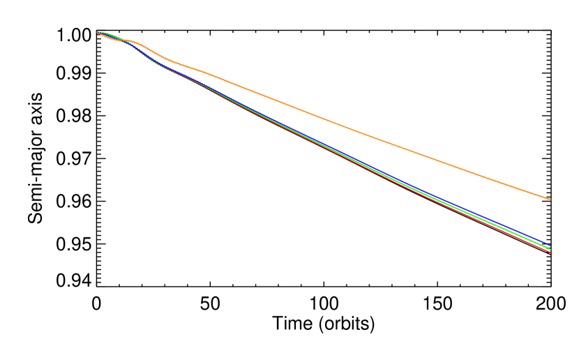
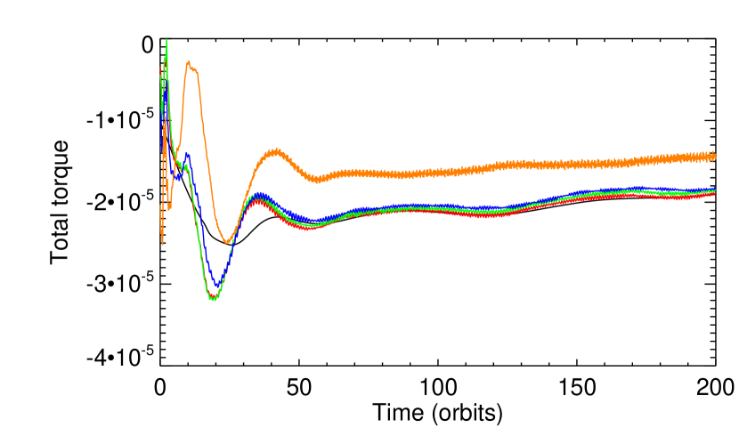
Figure 6: Upper panel: this figure shows the evolution of Saturn’s semi-major axis for the different sizes of the dead-zone we consider, namely for $H_{DZ}/H=0$ (black line), $H_{DZ}/H=0.5$ (red line), $H_{DZ}/H=1$ (green line), $H_{DZ}/H=1.5$ (blue line) and $H_{DZ}/H=2.3$ (orange line). Lower panel: this figure shows the corresponding total torque exerted on the planet.

Figure 7: Upper panel: this figure shows the radial distribution of the torque for the runs with $H_{DZ}=H$ and $H_{DZ}/H=2.3$. The planet is here located at $a=0.96$. Lower panel: this figure shows the vertical distribution of the torque in the upper disk layers.

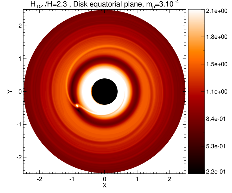
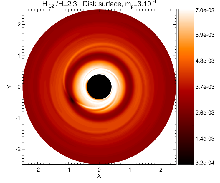
Figure 8: Left panet: this figure shows,for $H_{DZ}/H=2.3$, a snapshot of the disk density in the equatorial plane at a time where a planet held on a circular orbit at $R=1$ and with initial mass $m_{p}=30\;M_{\oplus}$ has grown to become a Saturn-mass planet. Right panel: same but at the disk surface.

4.3 Orbital evolution of Jupiter-mass planets

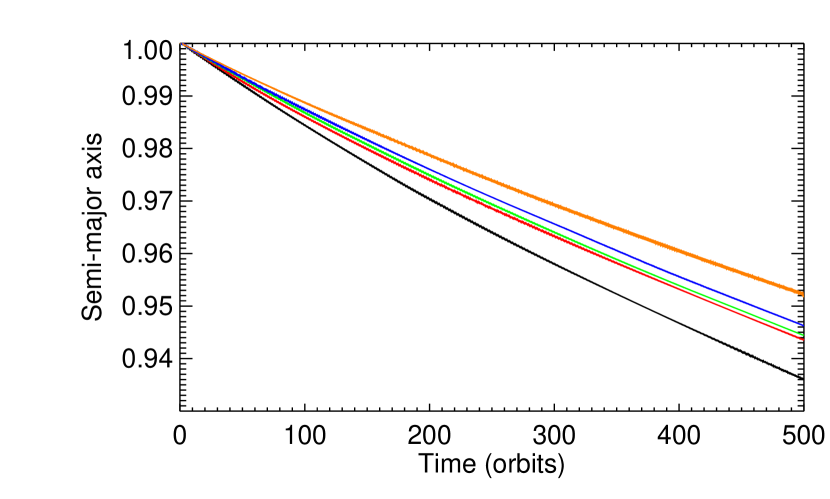
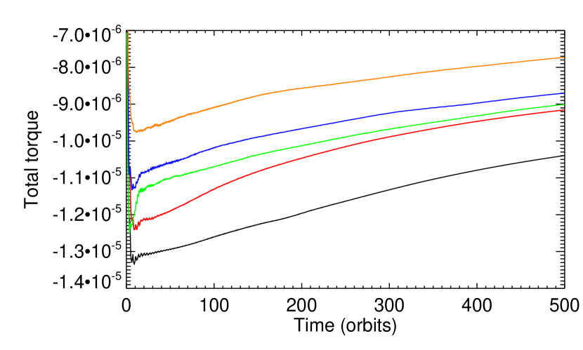
Figure 9: Upper panel: this figure shows the evolution of Jupiter’s semi-major axis for the different sizes of the dead-zone we consider, namely for $H_{DZ}/H=0$ (black line), $H_{DZ}/H=0.5$ (red line), $H_{DZ}/H=1$ (green line), $H_{DZ}/H=1.5$ (blue line) and $H_{DZ}/H=2.3$ (orange line). Lower panel: this figure shows the corresponding total torque exerted on Jupiter.

We now turn to the question of how the orbit of a Jupiter-mass planet evolves in a dead-zone. Here again, to address this issue, we restarted the simulations presented in Sect. 4.1 once the mass of the accreting protoplanet has reached $m_{p}=1\;M_{J}$, but we now let the planet evolve under the influence of the disk for $\sim 500$ orbits.
The time evolution of Jupiter’s semi-major axis is shown in the upper panel of Fig. 9. As expected, the planet migrates on a timescale corresponding to Type II migration in the case where $H_{DZ}/H=0$. For models with $H_{DZ}\neq 0$ however, we see here that, compared with the Saturn case, the dependency of the migration rate upon the value for $H_{DZ}$ is stronger, with a clear tendency for the semi-major axis to decrease more slowly as the size of the dead-zone increases. Examination of the total disk torques, which are represented in the lower panel of Fig. 9, clearly reveals that these decrease in magnitude with increasing the size of the dead-zone. The outer and inner torques exerted on the planet are displayed in the upper and lower panels of Fig. 10, respectively. Interestingly, and despite a weak dependency on the value for $H_{DZ}$, the presence of a dead-zone reduces the effects of the outer torques exerted on the planet. As illustrated in Fig. 11, which shows the disk surface density as a function of radius (at an azimuthal position corresponding to that of the planet), this arises because the surface density at the outer edge of the gap is greater in the case where $H_{DZ}=0$ compared to cases where $H_{DZ}>0$, increasing the magnitude of the outer torques. Moreover, Fig. 11 reveals that the density in the inner disk is much more higher for the simulation with $H_{DZ}=2.3H$, which consequently favours the higher positive torque exerted on the planet in this case (see the lower panel of Fig. 10). It should be noted that for models with $H_{DZ}\neq 0$, and provided that the viscosity is high enough in the live-zone, a migration rate which is lower than the inward drift velocity in the active region can make the disk material from this region flow across the gap. This not only enables the inner disk to be continuously supplied with gas but also creates a positive corotation torque on the planet as the gas flows through the gap (Masset & Snellgrove 2001; Morbidelli & Crida 2007).

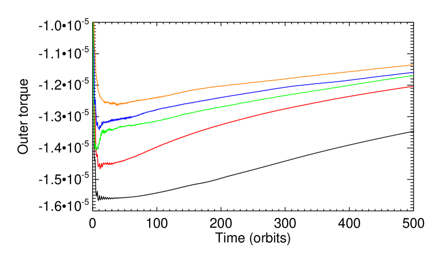
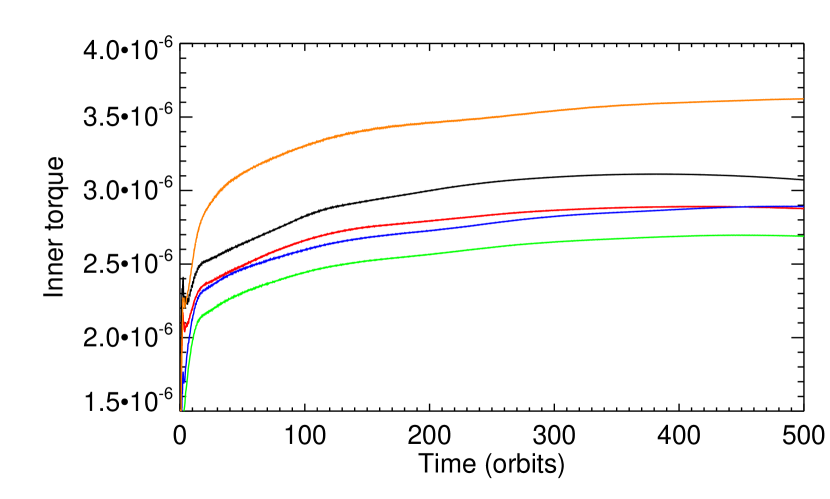
Figure 10: Upper panel: this figure shows the time evolution of the outer torque exerted on Jupiter, for the different sizes of the dead-zone we consider,namely for $H_{DZ}/H=0$ (black line), $H_{DZ}/H=0.5$ (red line), $H_{DZ}/H=1$ (green line), $H_{DZ}/H=1.5$ (blue line) and $H_{DZ}/H=2.3$ (orange line). Lower panel: same but for the inner torque.

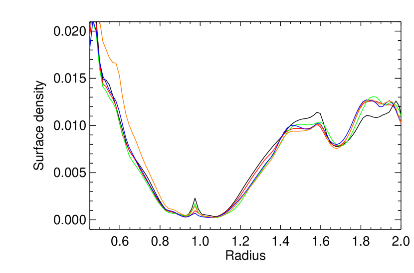
Figure 11: This figure shows, for the simulations in which $m_{p}=10^{-3}$, the disk surface density as a function of radius and for an azimuthal position corresponding to that of the planet. Different sizes of the dead-zone are considered, namely $H_{DZ}/H=0$ (black line), $H_{DZ}/H=0.5$ (red line), $H_{DZ}/H=1$ (green line), $H_{DZ}/H=1.5$ (blue line) and $H_{DZ}/H=2.3$ (orange line).

4.4 Planet evolution in an alternative dead-zone model

The prescription that we have used to model the variation of viscous stress in disks with dead-zones depends only on the height of the fluid from the disk midplane. It is possible that some of our results may be affected by this prescription, since the spatial extent of a dead-zone should probably depend on the local column density (assuming that external sources of ionisation such as cosmic rays or X-rays are responsible for ionising the disk). The assumption of a stationary profile for $\alpha$ is reasonable in a disk which remains largely unperturbed, but may become inaccurate when gaps form due to the presence of planets, since material near the midplane located in the gap should become magnetically active. To further investigate this issue, we have performed additional simulations using the following vertical profile for $\alpha$:

$$\alpha=\alpha_{0}(R)\exp\left(-\frac{\eta(z)}{\eta_{c}}\right)$$ (16)

where $\eta(z)=\int_{z}^{\infty}\rho dz^{\prime}$ is the column density at height $z$, and where $\alpha_{O}$ is determined in such a way that the vertically averaged mass flow through the disk is $\dot{M}_{0}$ at each radius. In the previous equation, we set $\eta_{c}=8.35\times 10^{-3}$ which corresponds to the initial value for the column density at altitude $z=1.5H$. The upper panel of Fig. 12 shows the azimutally-averaged vertical profile of the $\alpha$-parameter at $R=1$ for a simulation in which an initial $30\;M_{\oplus}$ protoplanet grows to become a Jupiter mass planet, and for which $\alpha$ is given by the previous equation. The solid line depicts the initial profile for $\alpha$, whereas the dashed and dot-dashed lines correspond to times at which $m_{p}=3\times 10^{-4}$ and $m_{p}=10^{-3}$, respectively. As the planet grows and is able to open a gap in the disk, the vertical profile of $\alpha$ at the position of the planet relaxes toward a uniform distribution with $\alpha=1.4\times 10^{-3}$ throughout the vertical extent of the disk. Although not presented here, it is worthwhile noting that for such a simulation, the time evolution of the planet mass is almost indistinguishable from that obtained using the prescription of Eq. 11, as the value for the mass accretion rate is the same.

For this model, the middle and lower panels of Fig. 12, respectively, display the evolution of the semi-major axes for the Saturn and Jupiter-mass planets. Compared with the previous model with $H_{DZ}=1.5H$, the migration of Saturn proceeds very similarly. This arises because in both cases, the value for the laminar viscosity in the active region is not high enough for the corotation torque to be unsaturated. In the Jupiter case, the difference between the two models after $200$ orbits is again marginal despite the fact that for the new model $\alpha$ is vertically constant at the position of Jupiter (see the upper panel of Fig. 12). This supports the idea that the prescription we adopt for $\alpha$ has little influence on the subsequent evolution of the planet.

5 Discussion and conclusion

In this paper we have presented the results of hydrodynamic simulations aimed at studying the effect of a dead-zone on the formation and evolution of giant planets. For layered disks we model the dead-zone as a region where the viscosity profile depends on the distance from the equatorial plane, and we considered different values for the dead-zone size, ranging from $H_{DZ}=0$ to $H_{DZ}=2.3H$. For each value of $H_{DZ}$, we focused on a model in which a $30\;M_{\oplus}$ protoplanet accretes gas from the disk until its mass reaches either $m_{p}=1\;M_{S}$ or $m_{p}=1\;M_{J}$. Once the final planet mass has been attained, we assumed that accretion stops, and let the planet evolve under the action of disk torques.
The results of our simulations indicate that, for a given mass accretion rate through the disk, the timescale over which a $30\;M_{\oplus}$ protoplanet grows to become a giant planet does not depend on the size of the dead-zone. This occurs because the planet is able to pull some of the gas from the live-zone down toward the midplane, from where it can be accreted, as the latter flows into the gap region. However, we find that the migration of giant planets can be modestly affected by the presence of a dead-zone. Indeed, there is a clear tendency for Jupiter-mass planets to migrate more slowly as the size of the dead-zone increases. For Saturn-mass planets, we find that although migration depends only weakly on the size of the dead-zone for models with $H_{DZ}\leq 1.5H$, it proceeds more slowly in the case where $H_{DZ}=2.3H$. This is due to the fact that in the latter case, the viscosity in the live-zone is high enough for the corotation torque to become unsaturated.

Although the present study suggests that a dead-zone does not have a significant impact on the growth and migration of giant planets, it will be of interest to examine this issue using three-dimensional MHD simulations, which include a dead-zone, in order to confirm (or refute) our findings. Of particular interest will be the issue of what happens when gap opening allows disk material in the vicinity of the planet to become magnetically active. We will address this issue in a future paper.

Figure 12: Upper panel: this figure displays the $\alpha$-parameter azimutally-averaged vertical profile at $R=1$ for a simulation in which an initial $30\;M_{\oplus}$ protoplanet grows to become a Jupiter-mass planet and in which $\alpha$ is given by Eq. 16. Different times are considered corresponding to times at which $m_{p}=9.10^{-5}$ (solid line), $m_{p}=3\times 10^{-4}$ (dashed line) and $m_{p}=10^{-3}$ (dash-dotted line). Middle panel: this figure shows the time evolution of Saturn’s semi-major axis, for a model in which $\alpha$ is given by Eq. 11 with $H_{DZ}/H=1.5$ (blue line) and for a simulation in which $\alpha$ is given by Eq. 16 (dashed line). Lower panel: same but for Jupiter.

References

- Balbus & Hawley (1991) Balbus, S. A., & Hawley, J. F. 1991, ApJ, 376, 214
- Beckwith (1996) Beckwith, S. V. W. 1996, Nature, 383, 139
- Blaes & Balbus (1994) Blaes, O. M., & Balbus, S. A. 1994, ApJ, 421, 163
- Brandenburg et al. (1996) Brandenburg, A., Nordlund, A., Stein, R. F., & Torkelsson, U. 1996, ApJ, 458, L45
- Bryden et al. (1999) Bryden, G., Chen, X., Lin, D. N. C., Nelson, R. P., & Papaloizou, J. C. B. 1999, ApJ, 514, 344
- de Val-Borro et al. (2006) de Val-Borro, M., et al. 2006, MNRAS, 370, 529
- Crida et al. (2006) Crida, A., Morbidelli, A., & Masset, F. 2006, Icarus, 181, 587
- Fleming & Stone (2003) Fleming, T., & Stone, J. M. 2003, ApJ, 585, 908
- Fromang et al. (2002) Fromang, S., Terquem, C., & Balbus, S. A. 2002, MNRAS, 329, 18
- Fromang & Nelson (2006) Fromang, S., & Nelson, R. P. 2006, A&A, 457, 343
- Fromang & Papaloizou (2006) Fromang, S., & Papaloizou, J. 2006, A&A, 452, 751
- Gammie (1996) Gammie, C. F. 1996, ApJ, 457, 355
- Greenberg et al. (1978) Greenberg, R., Wacker, J. F., Hartmann, W. K., & Chapman, C. R. 1978, Lunar and Planetary Institute Science Conference Abstracts, 9, 413
- Gullbring et al. (1998) Gullbring, E., Hartmann, L., Briceno, C., & Calvet, N. 1998, ApJ, 492, 323
- Haisch et al. (2001) Haisch, K. E., Jr., Lada, E. A., & Lada, C. J. 2001, ApJ, 553, L153
- Hartmann et al. (1998) Hartmann, L., Calvet, N., Gullbring, E., & D’Alessio, P. 1998, ApJ, 495, 385
- Hawley et al. (1996) Hawley, J. F., Gammie, C. F., & Balbus, S. A. 1996, ApJ, 464, 690
- Ilgner & Nelson (2006) Ilgner, M., & Nelson, R. P. 2006a, A&A, 445, 206
- Ilgner & Nelson (2006) Ilgner, M., & Nelson, R. P. 2006b, A&A, 445, 223
- Ilgner & Nelson (2008) Ilgner, M., & Nelson, R. P. 2008, A&A, 483, 815
- Leinhardt & Richardson (2005) Leinhardt, Z. M., & Richardson, D. C. 2005, ApJ, 625, 427
- Lovelace et al. (1999) Lovelace, R. V. E., Li, H., Colgate, S. A., & Nelson, A. F. 1999, ApJ, 513, 805
- Lyra et al. (2008) Lyra, W., Johansen, A., Klahr, H., & Piskunov, N. 2008, A&A, 491, L41
- Lyra et al. (2009) Lyra, W., Johansen, A., Zsom, A., Klahr, H., & Piskunov, N. 2009, A&A, 497, 869
- Kley (1999) Kley, W. 1999, MNRAS, 303, 696
- Kokubo & Ida (1998) Kokubo, E., & Ida, S. 1998, Icarus, 131, 171
- Kokubo & Ida (2000) Kokubo, E., & Ida, S. 2000, Icarus, 143, 15
- Klahr et al. (1999) Klahr, H. H., Henning, T., & Kley, W. 1999, ApJ, 514, 325
- Klahr & Bodenheimer (2003) Klahr, H. H., & Bodenheimer, P. 2003, ApJ, 582, 869
- Lin & Papaloizou (1986) Lin, D. N. C., & Papaloizou, J. 1986, ApJ, 309, 846
- Masset & Snellgrove (2001) Masset, F., & Snellgrove, M. 2001, MNRAS, 320, L55
- Masset (2002) Masset, F. S. 2002, A&A, 387, 605
- Masset & Papaloizou (2003) Masset, F. S., & Papaloizou, J. C. B. 2003, ApJ, 588, 494
- Masset et al. (2006) Masset, F. S., Morbidelli, A., Crida, A., & Ferreira, J. 2006, ApJ, 642, 478
- Masset et al. (2006) Masset, F. S., D’Angelo, G., & Kley, W. 2006, ApJ, 652, 730
- Matsumura & Pudritz (2003) Matsumura, S., & Pudritz, R. E. 2003, ApJ, 598, 645
- Meyer-Vernet & Sicardy (1987) Meyer-Vernet, N., & Sicardy, B. 1987, Icarus, 69, 157
- Morbidelli & Crida (2007) Morbidelli, A., & Crida, A. 2007, Icarus, 191, 158
- Nelson et al. (2000) Nelson, R. P., Papaloizou, J. C. B., Masset, F., & Kley, W. 2000, MNRAS, 318, 18
- Nelson & Papaloizou (2003) Nelson, R. P., & Papaloizou, J. C. B. 2003, MNRAS, 339, 993
- Nelson & Papaloizou (2004) Nelson, R. P., & Papaloizou, J. C. B. 2004, MNRAS, 350, 849
- Nelson (2005) Nelson, R. P. 2005, A&A, 443, 1067
- Papaloizou & Lin (1984) Papaloizou, J., & Lin, D. N. C. 1984, ApJ, 285, 818
- Papaloizou & Nelson (2003) Papaloizou, J. C. B., & Nelson, R. P. 2003, MNRAS, 339, 983
- Papaloizou et al. (2004) Papaloizou, J. C. B., Nelson, R. P., & Snellgrove, M. D. 2004, MNRAS, 350, 829
- Papaloizou & Nelson (2005) Papaloizou, J. C. B., & Nelson, R. P. 2005, A&A, 433, 247
- Pierens & Nelson (2008) Pierens, A., & Nelson, R. P. 2008, A&A, 482, 333
- Pollack et al. (1996) Pollack, J. B., Hubickyj, O., Bodenheimer, P., Lissauer, J. J., Podolak, M., & Greenzweig, Y. 1996, Icarus, 124, 62
- Sano et al. (2000) Sano, T., Miyama, S. M., Umebayashi, T., & Nakano, T. 2000, ApJ, 543, 486
- Sicilia-Aguilar et al. (2004) Sicilia-Aguilar, A., Hartmann, L. W., Briceño, C., Muzerolle, J., & Calvet, N. 2004, AJ, 128, 805
- Sicilia-Aguilar et al. (2006) Sicilia-Aguilar, A., et al. 2006, ApJ, 638, 897
- Shakura & Sunyaev (1973) Shakura, N. I., & Sunyaev, R. A. 1973, A&A, 24, 337
- Tanaka et al. (2002) Tanaka, H., Takeuchi, T., & Ward, W. R. 2002, ApJ, 565, 1257
- Thommes et al. (2003) Thommes, E. W., Duncan, M. J., & Levison, H. F. 2003, Icarus, 161, 431
- Turner & Drake (2009) Turner, N. J., & Drake, J. F. 2009, ApJ, 703, 2152
- Wetherill & Stewart (1989) Wetherill, G. W., & Stewart, G. R. 1989, Icarus, 77, 330
- (57) Ziegler, U., & Yorke, H. W., 1997, Comput. Phys. Commun, 101, 54