Unusual Thermodynamics on the Fuzzy 2-Sphere

Abstract:

Higher spin Dirac operators on both the continuum sphere($S^{2}$) and its fuzzy analog($S^{2}_{F}$) come paired with anticommuting chirality operators. A consequence of this is seen in the fermion-like spectrum of these operators which is especially true even for the case of integer-spin Dirac operators. Motivated by this feature of the spectrum of a spin 1 Dirac operator on $S_{F}^{2}$, we assume the spin 1 particles obey Fermi-Dirac statistics. This choice is inspite of the lack of a well defined spin-statistics relation on a compact surface such as $S^{2}$. The specific heats are computed in the cases of the spin $\frac{1}{2}$ and spin 1 Dirac operators. Remarkably the specific heat for a system of spin $\frac{1}{2}$ particles is more than that of the spin 1 case, though the number of degrees of freedom is more in the case of spin 1 particles. The reason for this is inferred through a study of the spectrums of the Dirac operators in both the cases. The zero modes of the spin 1 Dirac operator is studied as a function of the cut-off angular momentum $L$ and is found to follow a simple power law. This number is such that the number of states with positive energy for the spin 1 and spin $\frac{1}{2}$ system become comparable. Remarks are made about the spectrums of higher spin Dirac operators as well through a study of their zero-modes and the variation of their spectrum with degeneracy. The mean energy as a function of temperature is studied in both the spin $\frac{1}{2}$ and spin 1 cases. They are found to deviate from the standard ideal gas law in 2+1 dimensions.

1 Introduction

The fuzzy 2-sphere($S_{F}^{2}$) [1, 2] is an example of a noncommutative spacetime where the algebra of functions on the commutative 2-sphere($S^{2}$) is approximated by an associative matrix algebra. In principle this helps in regularizing field theories on such spaces, providing an alternative way to discretize spacetimes. The most non-trivial feature of this approach is the preservation of symmetries of the commutative spacetime even at the discrete level. Field theories on $S_{F}^{2}$ have been actively pursued in the last few years [3, 4, 5, 6]. Several works on numerical simulations of scalar fields and gauge fields on $S_{F}^{2}$ have also been done. [7, 8, 9, 10, 11, 12]. These works study phase transitions of scalar fields on the fuzzy sphere and they show the existence of new phases in the continuum which break translational as well as other global symmetries. The study of a real scalar field with a $\phi^{4}$ interaction reveals the existence of a non-uniform ordered phase which is similar to the striped phase [13, 14, 15]. This feature distinguishes it from its commutative counterpart. Apart from these novel phenomena one can also incorporate supersymmetry in a precise manner on $S_{F}^{2}$ [16].

Fuzzy spaces other than $S_{F}^{2}$ have also been seen in the context of topology change [17, 18]. Physics on other fuzzy spaces have also been considered [19, 20].

To add to these new features on $S_{F}^{2}$, in this paper we probe the thermodynamics of spin 1 and spin $\frac{1}{2}$ particles on the fuzzy sphere. We find several counterintuitive results which we will present in this work. We work with the spectrum of the Dirac operators for the spin 1 and spin $\frac{1}{2}$ case. This is natural to do as the Dirac operator is fundamental to physics and is useful in formulating metrical, differential geometric and bundle-theoretic ideas. Moreover in Connes’ approach to noncommutative geometry [21], the Dirac operator gains fundamental significance as part of the spectral triple in formulating the spectral action principle [22]. There are several ways to construct the Dirac operator on the fuzzy sphere [23, 24, 25, 26]. They construct the Dirac operator for a spin $\frac{1}{2}$ particle. In our approach we construct the Dirac operators using the Ginsparg-Wilson(GW) algebra [27]. Through this method we can extend the construction to all higher spins as studied in [28].

We consider the spin 1 Dirac operators constructed in [28]. Unlike the spin $\frac{1}{2}$ case, analytic computation of the spectrum of these operators are difficult. This lead us to compute its spectrum numerically [29]. Though we could not go to arbitrarily large values of the cut-off angular momenta $L$, we could still predict the spectrum’s behavior in the continuum by observing the striking patterns that emerged for the spectrums for the values we could compute for. In [28], 3 different Dirac operators along with 3 chirality operators were constructed for the spin 1 case. They are all unitarily inequivalent as proved in [29]. We consider only the spectrum of the traceless spin 1 Dirac operator in this work.

Using this spectrum we first compute the partition function for a system of spin 1 particles on $S_{F}^{2}$. For doing this we need to assume the particles obey a particular statistics. As we are dealing with a chiral system we assume that the particles obey the Fermi-Dirac statistics. However it should be noted that the conventional proofs of the spin-statistics theorem hold in relativistic quantum field theories(qft’s) in three or more dimensions. They use the axioms of local relativistic qft’s. For comprehensive proofs see [30, 31]. Field theory on the fuzzy sphere is not a relativistic one as the symmetry group of the underlying theory is $SU(2)$. This being the case there is no well defined spin-statistics relation on the fuzzy sphere. However there are spin statistics relations which do not require relativity and which are topological [32, 33, 34]. General theory for quantum statistics in 2 spatial dimensions have also been discussed [35]. The non-triviality in two spatial dimensions arises due to topology of the configuration space of indistinguishable particles living on such a space. The fundamental group for such a configuration space($\frac{(\mathbb{R}^{2})^{N}-{\Delta}}{S_{N}}$, where ${\Delta}={(\vec{r}_{1},\vec{r}_{2},...,\vec{r}_{N})|\vec{r}_{i}\in\mathbb{R}^{2}\textrm{and}~{}\vec{r}_{i}=\vec{r}_{j}}$ for some $i\neq j$ and $S_{N}$ is the symmetric group of $N$ particles.) is the braid group $B_{N}$. For the case of $S^{2}$ instead of $\mathbb{R}^{2}$, the fundamental group is still the braid group with an additional constraint [36, 37]. These considerations allow for the possibility of the assumption of anyonic statistics [35, 38, 39, 40] in our case, but we do not consider these possibilities in this work and only briefly remark about them in the final section.

The main result of this paper is the mean energy of the spin $\frac{1}{2}$ system is more than that of the spin 1 system. This is surprising given the fact that there are more number of states possible in the spin 1 case, $3\times(2L+1)^{2}$ than in the spin $\frac{1}{2}$ case, $2\times(2L+1)^{2}$. Nevertheless we come to terms with this strange behavior by looking at the distribution of the eigenvalues of the Dirac operators in both the cases. In particular the spectrum of the spin 1 Dirac operator consists of a number of zero modes which are absent in the spin $\frac{1}{2}$ case. These characteristics provide an answer to the strange behavior of the mean energies. A consequence of this is also seen in the specific heats of the two systems. The entropy of the spin $\frac{1}{2}$ system is also more than the spin 1 system.

The other result is the deviation of the plot of the mean energy vs temperature from the corresponding curve for an ideal gas on a two dimensional space. The mean energy of an ideal gas of massless particles on a flat two dimensional space goes as $T^{3}$. We find a deviation from this law which is attributed to the dispersion relation of the spin $\frac{1}{2}$ and spin 1 systems on the 2-sphere.

The paper is organized as follows. Section 2 reviews the noncommutative algebra of functions on $S_{F}^{2}$. The GW algebra and the construction of the Dirac operators are reviewed in section 3. In section 4 we describe a way to find the spectrum of the spin 1 Dirac operator for arbitrarily large cut-off $L$. This is done by looking at a particular scaling behavior found in their spectrum. The grand canonical partition function is computed in section 5. This is used to compute the mean energy and the specific heats for both the cases of spin 1 and spin $\frac{1}{2}$ systems. This section presents the relevant numerical results. Zero mode analysis is also carried out in this section along with the reasons for the strange behavior. We also speculate the behavior of the mean energies for higher spin Dirac operators. Section 6 discusses the deviation from ideal gas behavior of these systems. We conclude in section 7 with a few remarks.

2 Geometry of $S_{F}^{2}$

The algebra for the fuzzy sphere is characterized by a cut-off angular momentum $L$ and is the full matrix algebra $Mat(2L+1)\equiv M_{2L+1}$ of $(2L+1)\times(2L+1)$ matrices. They can be generated by the $(2L+1)$-dimensional irreducible representation (IRR) of $SU(2)$ with the standard angular momentum basis. The latter is represented by the angular momenta $L^{L}_{i}$ acting on the left on $Mat(2L+1)$: If $\alpha\in Mat(2L+1)$,

$${L_{i}^{L}\alpha=L_{i}\alpha}$$ (1)

$${[L_{i}^{L},L_{j}^{L}]=i\epsilon_{ijk}L_{k}^{L}}$$ (2)

$${(L_{i}^{L})^{2}=L(L+1)\mathbf{1}}$$ (3)

where $L_{i}$ are the standard angular momentum matrices for angular momentum $L$.

We can also define right angular momenta $L_{i}^{R}$:

$${L_{i}^{R}\alpha=\alpha L_{i},\alpha\in M_{2L+1}}$$ (4)

$${[L_{i}^{R},L_{j}^{R}]=-i\epsilon_{ijk}L_{k}^{R}}$$ (5)

$${(L_{i}^{R})^{2}=L(L+1)\mathbf{1}}$$ (6)

We also have

$${[L_{i}^{L},L_{j}^{R}]=0.}$$ (7)

The operator $\mathcal{L}_{i}=L_{i}^{L}-L_{i}^{R}$ is the fuzzy version of orbital angular momentum. They satisfy the $SU(2)$ angular momentum algebra

$${[\mathcal{L}_{i},\mathcal{L}_{j}]=i\epsilon_{ijk}\mathcal{L}_{k}}$$ (8)

In the continuum, $S^{2}$ can be described by the unit vector $\hat{x}\in S^{2}$, where $\hat{x}.\hat{x}=1$. Its analogue on $S_{F}^{2}$ is $\frac{L_{i}^{L}}{L}$ or $\frac{L_{I}^{R}}{L}$ such that

$${\lim_{L\rightarrow\infty}\frac{L_{i}^{L,R}}{L}=\hat{x}_{i}.}$$ (9)

This shows that $L_{i}^{L,R}$ do not have continuum limits. But $\mathcal{L}_{i}=L_{i}^{L}-L_{i}^{R}$ does and becomes the orbital angular momentum as $L\rightarrow\infty$:

$${\lim_{L\rightarrow\infty}L_{i}^{L}-L_{i}^{R}=-i(\overrightarrow{r}\wedge\overrightarrow{\nabla})_{i}.}$$ (10)

3 Construction of the Dirac Operators

In algebraic terms, the GW algebra $\mathcal{A}$ is the unital $\ast$ algebra over $\mathbf{C}$ ,generated by two $\ast$-invariant involutions $\Gamma,\Gamma^{\prime}$.

$$\mathcal{A}=\{\Gamma,\Gamma^{\prime}\ :\Gamma^{2}=\Gamma^{\prime 2}=1\ ,\Gamma^{*}=\Gamma\ ,\Gamma^{\prime*}=\Gamma^{\prime}\}$$ (11)

In any $\ast$ -representation on a Hilbert space, $\ast$ becomes the adjoint ${\dagger}$.

Consider the following two elements constructed out of $\Gamma,\Gamma^{\prime}$:

$${\Gamma_{1}=\frac{1}{2}(\Gamma+\Gamma^{\prime}),}$$ (12)

$${\Gamma_{2}=\frac{1}{2}(\Gamma-\Gamma^{\prime}).}$$ (13)

It follows from Eq.(11) that $\{\Gamma_{1},\Gamma_{2}\}=0$. This suggests that for suitable choices of $\Gamma$, $\Gamma^{\prime}$, one of these operators may serve as the Dirac operator and the other as the chirality operator provided they have the right continuum limits after suitable scaling.

For the spin $1$ case the combination which leads to the desired Dirac and chirality operators were found in [28] and they are

$${D_{1}=L\left(\frac{\Gamma_{L+1}^{L}-\Gamma_{L-1}^{R}}{2}\right),}$$ (14)

$${D_{2}=L\left(\frac{\Gamma_{L-1}^{L}-\Gamma_{L+1}^{R}}{2}\right)}$$ (15)

and

$${D_{3}=L\left(\frac{\Gamma_{L}^{L}-\Gamma_{L}^{R}}{2}\right).}$$ (16)

with

$${\gamma_{1}=\left(\frac{\Gamma_{L+1}^{L}+\Gamma_{L-1}^{R}}{2}\right),}$$ (17)

$${\gamma_{2}=\left(\frac{\Gamma_{L-1}^{L}+\Gamma_{L+1}^{R}}{2}\right)}$$ (18)

and

$${\gamma_{3}=\left(\frac{\Gamma_{L}^{L}+\Gamma_{L}^{R}}{2}\right)}$$ (19)

as their corresponding chirality operators. In the above equations

$${\Gamma_{L+1}^{L}=\frac{2(\vec{\Sigma}.\vec{L}^{L}+L+1)(\vec{\Sigma}.\vec{L}^{L}+1)-(L+1)(2L+1)}{(L+1)(2L+1)},}$$ (20)

$${\Gamma_{L+1}^{R}=\frac{2(-\vec{\Sigma}.\vec{L}^{R}+L+1)(-\vec{\Sigma}.\vec{L}^{R}+1)-(L+1)(2L+1)}{(L+1)(2L+1)},}$$ (21)

$${\Gamma_{L-1}^{L}=\frac{2(\vec{\Sigma}.\vec{L}^{L}-L)(\vec{\Sigma}.\vec{L}^{L}+1)-L(2L+1)}{L(2L+1)},}$$ (22)

$${\Gamma_{L-1}^{R}=\frac{2(\vec{\Sigma}.\vec{L}^{R}+L)(\vec{\Sigma}.\vec{L}^{R}-1)-L(2L+1)}{L(2L+1)},}$$ (23)

$${\Gamma^{L}_{L}=\frac{-2(\vec{\Sigma}.\vec{L}^{L}-L)(\vec{\Sigma}.\vec{L}^{L}+L+1)-L(L+1)}{L(L+1)},}$$ (24)

and

$${\Gamma^{R}_{L}=\frac{2(\vec{\Sigma}.\vec{L}^{R}+L)(-\vec{\Sigma}.\vec{L}^{R}+L+1)-L(L+1)}{L(L+1)}.}$$ (25)

The operators in Eq.(20)-Eq.(25) are generators of GW algebras and are obtained from left and right projectors to eigenspaces of the total angular momentum, $\vec{L}+\vec{\Sigma}$, where $\vec{\Sigma}$ are the matrices representing the spin $1$ representation of $SU(2)$.

The continuum limits of Eq.(14)-Eq.(16) are

$${D_{1}=(\vec{\Sigma}.\vec{\mathcal{L}}-(\vec{\Sigma}.\hat{x})^{2}+2)+2(\vec{\Sigma}.\hat{x})+\{\vec{\Sigma}.\vec{\mathcal{L}},\vec{\Sigma}.\hat{x}\},}$$ (26)

$${D_{2}=(\vec{\Sigma}.\vec{\mathcal{L}}-(\vec{\Sigma}.\hat{x})^{2}+2)-2(\vec{\Sigma}.\hat{x})-\{\vec{\Sigma}.\vec{\mathcal{L}},\vec{\Sigma}.\hat{x}\}}$$ (27)

and

$${D_{3}=\vec{\Sigma}.\vec{\mathcal{L}}-(\vec{\Sigma}.\hat{x})^{2}+2.}$$ (28)

The corresponding chirality operators in the continuum are

$${\gamma_{1}=(\vec{\Sigma}.\hat{x})^{2}+(\vec{\Sigma}.\hat{x})-1,}$$ (29)

$${\gamma_{2}=(\vec{\Sigma}.\hat{x})^{2}-(\vec{\Sigma}.\hat{x})-1}$$ (30)

and

$${\gamma_{3}=1-2(\vec{\Sigma}.\hat{x})^{2}}$$ (31)

respectively.

4 Spectrum of the Spin 1 Dirac operator for large $N$

For a given cut-off $L=(N-1)/2$, the eigenvalues of the spin $\frac{1}{2}$ Dirac operator is given by $\pm(j+\frac{1}{2})$ where $j$ is the eigenvalue of the total angular momentum. The degeneracy $(g)$ of each of these eigenvalues $(E)$ is given by

$${g=2j+1.}$$ (32)

This gives the relation between the energy eigenvalue and its degeneracy as

$${E_{\frac{1}{2}}=\pm\frac{g}{2}.}$$ (33)

In contrast, the spin 1 system is richer with varied eigenvalues for each $L$ including a number of zero modes. Though we cant find the corresponding relation between the energy eigenvalue $E$ and its degeneracy $g$ analytically we can do so numerically [29].

The numerical results show that $g$ increases with $E$ for small values of $E$. After reaching a maximum for an intermediate value of $E$, $g$ decreases with $E$. This is unlike the spin $\frac{1}{2}$ case where $g$ is linear in $E$. After rotation (around origin, by a fixed angle) the plot of $E^{\prime}$ vs $g^{\prime}$ fits perfectly with a parabola. The rotation angle was found to be cut-off independent. Encouraged by this we tried to find if there is any universality in $E^{\prime}$ vs $g^{\prime}$. We found that results for different cut-off lie on a universal curve. This is done by scaling $E^{\prime}$ and $g^{\prime}$ so that the minimum of different curves match. In figure.1 one can see the results for $N=21,27$ and $45$ lie on top of each other after scaling. This result strongly suggest that we can obtain the spectrum for arbitrarily larger cut-off $(N)$ if we know the scaling variables for different $N$ [29]. The universality also suggests that $E^{\prime}$ vs $g^{\prime}$ is described by only two independent parameters. Once we know $E^{\prime}$ vs $g^{\prime}$ we rotate it to get the relation between $E$ and $g$, which is given by

$${E_{1}=\frac{\sqrt{b(g)^{2}-4ac(g)}-b(g)}{2a}}$$ (34)

where

$${a=\alpha\cos^{2}\theta,}$$ (35)

$${b(g)=2\alpha\cos\theta(\sin\theta g+\eta)+\sin\theta,}$$ (36)

$${c(g)=\alpha(\sin\theta g+\eta)^{2}+\beta-\cos\theta g}$$ (37)

and

$${\theta=2.26159~{}\textrm{radians}.}$$ (38)

As discussed above only $\beta(N)$ and $\eta(N)$ are independent parameters. For $\alpha$ we need to know its value for a particular $N$. For all other values of $N$, $\alpha$ can be calculated using $\beta(N)$ and $\eta(N)$.

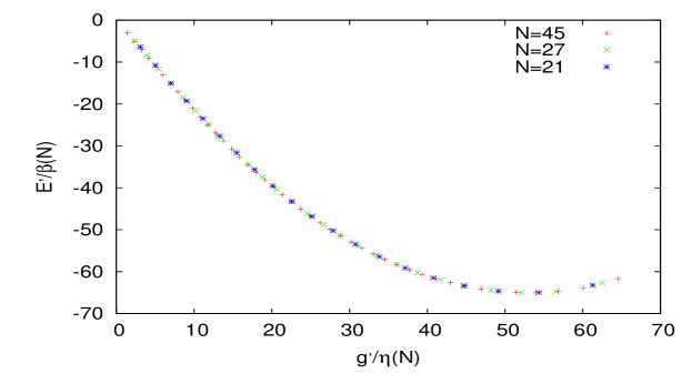
Figure 1: Scaling property of the spectrum of the spin 1 Dirac operator.

5 Numerical Results: I

5.1 The Partition Function and the Mean Energy

As explained in the introduction, we assume the spin 1 particles to obey fermionic statistics. The grand-canonical partition function is given by

$${lnZ=\sum_{i=1}g_{i}ln\left(1+e^{-\beta(E_{i}-\mu)}\right)}$$ (39)

where $g_{i}$ is the degeneracy of the ith level, $E_{i}$ is the energy of the ith level, $\mu$ is the chemical potential and $\beta=\frac{1}{k_{B}T}$. In the commutative case when there is no cut-off, the product over $i$ extends till infinity, but here we are restricted by the cut-off angular momentum $L$.

For the spin 1 case we numerically computed the spectrum of the Dirac operator given by Eq.(16) in [29]. We do not know how to find an analytic expression for the spectrum and so we compute the partition function numerically. (See however [29] for an analytic expression for the spectrum of the spin 1 Dirac operator derived as a result of the numerical computations.) The analogous situation for the spin $\frac{1}{2}$ case is fa better as we know its complete spectrum analytically for arbitrarily large cut-off $L$.

From the grand-canonical partition function in Eq.(39) we can use the standard formula to compute the mean energy which is

$${\langle E_{1}\rangle=-\frac{\partial lnZ}{\partial\beta}=\sum_{i=1}^{(2L+1)^{2}-1}\frac{g_{i}E_{i}}{e^{\beta(E_{i}-\mu)}+1}.}$$ (40)

In what follows we take the Boltzmann constant $k_{B}=1$ and the chemical potential $\mu=0$. The above expression for the mean energy is used for both the spin 1 and the spin $\frac{1}{2}$ cases. For the spin $\frac{1}{2}$ case it becomes

$${\langle E_{\frac{1}{2}}\rangle=\sum_{j=1}^{2L-\frac{1}{2}}\frac{1}{2}\frac{(2j+1)^{2}}{e^{\beta(j+\frac{1}{2})}+1}.}$$ (41)

Note that in the above Eqns.(40, 41) the sums are restricted by the cut-off $L$. The mean energies for both the cases were computed for various temperatures from 0.1 to 50. We show only these plots here though we did go to higher values of temperature and found nothing new. The plot for the mean energies of both the spin 1 and spin $\frac{1}{2}$ systems is shown in figure 2. The value of cut-off is $L=\frac{59}{2}$.

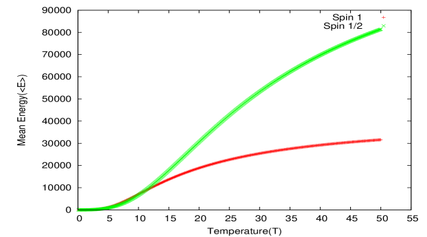
Figure 2: The mean energies of the spin 1 and spin $\frac{1}{2}$ systems.

In figure 2, the green curve shows the mean energy for the spin $\frac{1}{2}$ system as a function of temperature and the red one shows the corresponding curve for the spin 1 system. The curves become flat for higher values of temperature. This is due to the presence of the cut-off angular momentum in our sum. If we go to higher values of temperature this flattening occurs towards the higher temperatures considered. The plot clearly shows that the mean energy of the spin $\frac{1}{2}$ system is much higher than the spin 1 system. This is inspite of the spin 1 system having more number of degrees of freedom than the spin $\frac{1}{2}$ system. We know of no such analogous behavior in higher dimensions.

Another interesting feature in the behavior of these curves is the crossing of the two curves for low values of temperature. This is not clear in figure 2 but is shown explicitly in figure 3. This plot shows that the mean energy of the spin $\frac{1}{2}$ system is smaller than the spin 1 system till about $T=10.77$ after which it stays above the spin 1 curve.

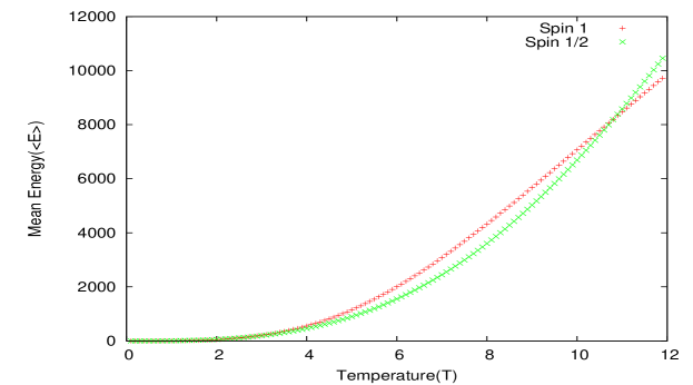
Figure 3: The crossing of the mean energy curves of the spin 1 and spin $\frac{1}{2}$ systems.

We now try to explain the cause of this unusual behavior by looking closely at the distributions of the eigenvalues of the Dirac operators of the two systems.

5.2 Reasons for the strange behavior

The main reason can be understood once we look at the spectrum of the Dirac operator in the two cases.

Using the expressions for the energy as a function of the degeneracy we can study the differences between the two systems. The relation is given by Eq.(33) for the spin $\frac{1}{2}$ case and Eq.(34) for the spin 1 case.

This plot of the energy eigenvalues as a function of their degeneracies is shown in figure 4.

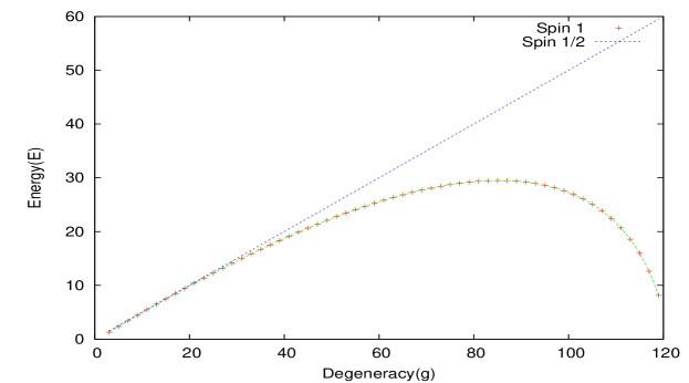
Figure 4: Energy as a function of the degeneracy $g$ for the spin $\frac{1}{2}$ and spin 1 systems.

For a given cut-off $L$, figure 4 clearly indicates that eigenvalues of the spin $\frac{1}{2}$ Dirac operator exceeds that of the spin 1 Dirac operator except for small values of the degeneracy $g$. The plot in figure 4 is shown only for positive values of the energy eigenvalue $E$. In the spin $\frac{1}{2}$ case the energy eigenvalues linearly increase with the degeneracy $g$ and so the maximum eigenvalue occurs for the $j$ value $2L-\frac{1}{2}$. We have ignored the maximum $j$ value of $2L+\frac{1}{2}$ as they correspond to unpaired eigenstates of the Dirac operator, which will be inconsistent given the chirality of the spin $\frac{1}{2}$ system squares to 1. This is a feature of the operator $\vec{\sigma}.\vec{\mathcal{L}}$ in the spin $\frac{1}{2}$ Dirac operator which is

$${D_{\frac{1}{2}}=\vec{\sigma}.\vec{\mathcal{L}}+\frac{1}{2},}$$ (42)

where $\vec{\sigma}$ are the Pauli matrices.

In the spin 1 case the maximum eigenvalue is $L$ and this occurs for some intermediate value of the degeneracy $g$ as can be seen in figure 4. The reason why the spin 1 Dirac operator consists of all eigenvalues ranging from $-L$ to $+L$ for a given $L$ can be seen by looking at the operator in the continuum given by Eq.(28) which we write here again:

$${D_{3}=\vec{\Sigma}.\vec{\mathcal{L}}-(\vec{\Sigma}.\hat{x})^{2}+2}$$ (43)

where $\vec{\Sigma}$ are the matrices of the spin 1 representation of $SU(2)$. The term $\vec{\Sigma}.\hat{x}$ makes the analytic computation of the spectrum in the spin 1 case difficult when compared to the spin $\frac{1}{2}$ case. We believe this term to be also the cause of the varied spectrum of the spin 1 system.

5.3 Zero modes of the spin 1 Dirac operator

The spectrum of the spin 1 Dirac operator consists of a number of zero modes for each cut-off angular momentum $L$. The number of such zero eigenvalues follows a simple power law as a function of $L$. This number was found to be $(2L+1)^{2}+2$. This is an exact result and can be found analytically as explained in [29]. This has also been verified numerically. With this result it follows immediately that the number of positive eigenvalues of the spin 1 system are $(2L+1)^{2}-1$. The spin $\frac{1}{2}$ Dirac operator has no zero modes as it has non-zero trace. Removing the states corresponding to the top mode gives us $4L^{2}+2L$ states with positive eigenvalues. The zero modes in the spin 1 case drastically reduce the total number of states corresponding to positive eigenvalues to $(2L+1)^{2}-1$ but this is still more than the corresponding number of states in the spin $\frac{1}{2}$ case.

The counting of the zero modes and the behavior of the spectrum with degeneracy in the two cases justify the counter-intuitive behavior of the mean energies.

We now digress a bit to remark about the plot in figure 4. We try to speculate the energy versus degeneracies curves for higher spin Dirac operators. To do this we first find the number of zero modes for higher spin Dirac operators. We will compute this for the integer spin case.

To construct higher spin Dirac operators on $S_{F}^{2}$, we need to construct operators acting on $Mat(2L+1)\otimes\mathbb{C}^{2k+1}$ where $k$ is the desired spin. The spectrum of these operators will in general be hard to compute due to the presence of $\vec{\Sigma}.\hat{x}$ terms just as in the spin 1 case.

The analytic computation of the number of zero modes was given in [29]. We extend those arguments to higher spins in the following. Consider the spectrum of the total angular momentum $j$ for a given cut-off $L$:

$${\textrm{Spec}~{}\vec{J}\in\{0,1,2,\cdots,2L-k,\cdots,2L,\cdots,2L+k\}.}$$ (44)

For an even-integer spin $k$, the number of zero-modes can be found by computing the following sum

$${\sum_{j=0}^{2L-k}(2j+1)+\sum_{j=-\frac{k-2}{2}}^{\frac{k}{2}}\left[2(2L+2j)+1\right]=(2L+1)^{2}+k^{2}+k.}$$ (45)

For an odd-integer spin $k$, this number is

$${\sum_{j=0}^{2L-k-1}(2j+1)+\sum_{j=-\frac{k+1}{2}}^{\frac{k-1}{2}}\left[2(2L+2j+1)+1\right]=(2L+1)^{2}+k^{2}+k.}$$ (46)

These computations hold as there exists a traceless Dirac operator for all integer spin Dirac operators on $S_{F}^{2}$. This is because we can construct an integer spin Dirac operator from the following combination of generators of GW algebra [28]:

$${D_{k}=L\left(\frac{\Gamma_{L}^{L}-\Gamma_{L}^{R}}{2}\right).}$$ (47)

As $tr(\Gamma_{L}^{L})=tr(\Gamma_{L}^{R})$, this operator is traceless.

In the case of the Dirac operators for half-integral spins, there exists no such combinations of generators of GW algebras which have 0 trace. This makes the number of states with positive energy eigenvalues for spin $k$ and spin $k-\frac{1}{2}$, for integer $k$, comparable.

We can then go on to compute their mean energies and compare them. We suspect $\langle E_{k-\frac{1}{2}}\rangle>\langle E_{k}\rangle$ to hold but we have no analytic proof for this. We could however compute the spectrums for the two Dirac operators numerically and carry out this comparison, but we do not do this here and save it for future work.

The reason why this is interesting is the following. It seems from the plot in figure 4 that the behavior of $\frac{E}{g}$ for small values of $g$ is similar for higher spins as well. We leave this as a conjecture as we have no analytic proof for this but do have strong reasons to suspect so.

It is also very likely that the plots of $E$ versus $g$ for higher spins will fall below the $E=\frac{g}{2}$ curve. This is expected due to the fact that higher spin Dirac operators contain $\vec{\Sigma}.\hat{x}$ terms along with $\vec{\Sigma}.\vec{\mathcal{L}}$ [28]. $\vec{\Sigma}$ is the $2k+1$ dimensional representation of $SU(2)$ for some spin $k$. The $\vec{\Sigma}.\hat{x}$ term disrupts the linearity between the energy and degeneracy. It is easy to see this as a linear relation between the energy and the degeneracy is only possible for a Dirac operator which has just a $\vec{\Sigma}.\vec{\mathcal{L}}$ term apart from constant terms. This can be seen analytically for any given spin $k$ by looking at the spectrum of $\vec{\Sigma}.\vec{\mathcal{L}}$:

$${\textrm{Spec}~{}\vec{\Sigma}.\vec{\mathcal{L}}=(k-m)(2j-k+m)-k^{2}-m~{}~{}m\in\{0,1,\cdots,2k\}.}$$ (48)

Only the spin $\frac{1}{2}$ Dirac operator contains just the $\vec{\sigma}.\vec{\mathcal{L}}$ term leading to the linear relation between its energy and their multiplicities.

The $\vec{\Sigma}.\hat{x}$ terms are present in the spin 1 case and it was remarked that these terms cause the energy versus degeneracy curve in figure 4. As these terms also occur for higher spin Dirac operators we expect a similar behavior from these systems. The reason why they occur for all higher spin Dirac operators is because of the fact that the fuzzy versions of these higher spin Dirac operators contain terms of the form

$$\frac{(\vec{\Sigma}.\vec{L^{L}})^{n}-(\vec{\Sigma}.\vec{L^{R}})^{n}}{L^{n-1}}.$$

The continuum limit of these terms contain $\vec{\Sigma}.\hat{x}$ terms. This is explained in detail in [28].

The preceding statements prove the non-linearity between the energy and their degeneracies for all Dirac operators other than the spin $\frac{1}{2}$ system. They however do not show that these curves fall below the corresponding curve for the spin $\frac{1}{2}$ system. A complete answer to this question would only come from a numerical analysis of this system and at present we leave this question as a worthy one to explore in the future.

5.4 Specific heats of the two systems

The specific heat is defined as the derivative of the mean energy with respect to temperature. A straightforward computation gives the specific heat as

$${C_{v}=\frac{1}{T^{2}}\sum_{i}\frac{g_{i}E_{i}^{2}e^{\beta E_{i}}}{(e^{\beta E_{i}}+1)^{2}}.}$$ (49)

As expected here too we find the specific heat of the spin $\frac{1}{2}$ system to be more than that of the spin 1 system. This is shown in figure 5.

There is a region till $T=10.77$ where the specific heat of the spin 1 system is more than that of the spin $\frac{1}{2}$ system. This can be seen as a result of the crossing of the mean energy curves for the two systems as shown in figure 3.

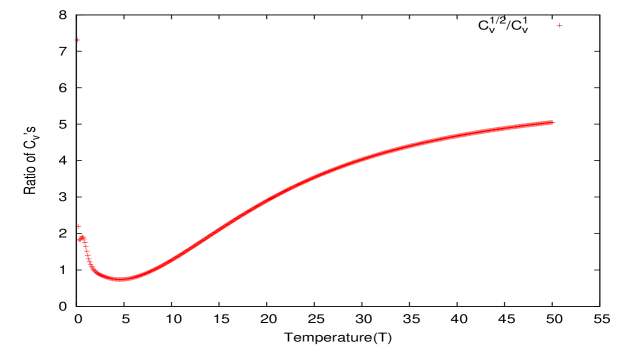
Figure 5: Ratio of specific heats $\frac{C_{v}^{\frac{1}{2}}}{C_{v}^{1}}$

5.5 Entropies of the two systems

The entropy is given by the equation

$${S=\sum_{i}g_{i}ln\left(1+e^{-\beta E_{i}}\right)+\frac{1}{T}\sum\frac{E_{i}}{1+e^{-\beta E_{i}}}.}$$ (50)

This follows from

$${S=lnZ+\beta\langle E\rangle.}$$ (51)

From these formulas it can be easily seen that the entropy of a spin 1 system is less than that of a spin $\frac{1}{2}$ system.

6 Numerical Results: II

6.1 Deviations from the Ideal Gas Law

For a system of non-interacting massless particles obeying Fermionic statistics, the mean energy goes as $T^{4}$ in 3+1 dimensions. This can be seen as follows:

$${\langle E\rangle=\int d^{3}p\frac{p}{e^{\beta p}+1}}$$ (52)

where $p$ is the energy of the massless particle. This is the dispersion law for a massless particle on a flat space which has the Poincare group has its group of symmetries. We now substitute

$$x=\frac{p}{T}$$

to find

$${\langle E\rangle\propto T^{4}\int_{0}^{\infty}dx\frac{x^{3}}{e^{x}+1}.}$$ (53)

In a similar manner, in 2+1 dimensions, the mean energy goes as $T^{3}$. This law holds however only for a system living on a flat 2+1 dimensional spacetime.

In the case of the spin $\frac{1}{2}$ system living on $S^{2}$ or $S_{F}^{2}$ the mean energy is given by

$${\langle E_{\frac{1}{2}}\rangle=\sum_{j=0}^{2L+\frac{1}{2}}\frac{1}{2}\frac{(2j+1)^{2}}{e^{\frac{2j+1}{2T}}+1}.}$$ (54)

We have cut-off the sum with a cut-off $L$. If we arbitrarily increase the value of the cut-off $L$ we will find the sum replaced by an integral over $j$ and the upper limit in the sum goes to $\infty$. In the above equation make the substitution

$${\frac{2j+1}{T}=x.}$$ (55)

This makes the sum

$${\langle E_{\frac{1}{2}}\rangle=\frac{T^{2}}{2}\sum_{x=\frac{1}{T}}^{\frac{4L+2}{T}}\frac{x^{2}}{e^{\frac{x}{2}}+1}.}$$ (56)

As the limits of the sum depend on the temperature $T$ we get no definite relation between the mean energy and temperature. It should be noted that the upper limit is dependent on $T$ due to the cut-off $L$. We can remove this by allowing $L$ to go to $\infty$. In such a case, as already mentioned the sum becomes an integral making the dependence go as $T^{3}$. This still does not remove the $T$ dependence from the lower limit of the integral. This is due to the dispersion relation for the spin $\frac{1}{2}$ particle which goes as $j+\frac{1}{2}$. The additional $\frac{1}{2}$ can be attributed to the curvature of the sphere the system lives on. This results in the deviation from ideal gas law on 2+1 dimensional space.

Similar arguments hold for the spin 1 case also. This can be easily seen from our analytic expressions for the spectrum of the spin 1 Dirac operator as seen in the previous section. We do not write the simple details of this here.

The deviations for the spin $\frac{1}{2}$ and the spin 1 system are shown in the plots in figures 6 and 7.

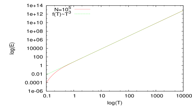
Figure 6: Deviation from ideal gas law for the spin $\frac{1}{2}$ system.

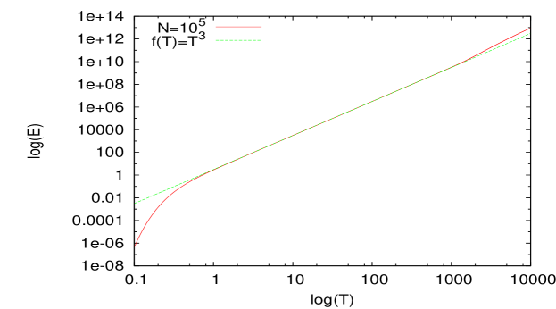
Figure 7: Deviation from the ideal gas law for the spin 1 system.

7 Conclusions

Spin systems on the fuzzy 2-sphere show several interesting features as discussed in this paper. The main result being the mean energy of a spin $\frac{1}{2}$ system is greater than that of a spin 1 system. This is a novel phenomenon with no known higher dimensional analog. Its implications are worth exploring. The simple power law of the zero modes is another remarkable feature of these systems.

Speculations were made about the spectrums of higher spin Dirac operators on $S_{F}^{2}$. Though we could not arrive at a concrete result, we conjectured that it is likely that the mean energy of the spin $\frac{1}{2}$ system will be more than that of the mean energies of other spins greater than $\frac{1}{2}$. This gives an upper bound on the mean energy of these spin systems on $S_{F}^{2}$. This bound will also translate to the entropies of these systems, thus making the entropies of these spin systems to be bounded by the entropy of the spin $\frac{1}{2}$ system. This would mean that an increase in the number of states on $S_{F}^{2}$ have no effect on the entropy, a property very much reminiscent of the holographic principle though there is no bulk theory involved here. This is conjectural and we plan to explore this in the future.

The deviation from the ideal gas law is another interesting phenomenon in this fuzzy system. It can definitely serve as a model for explaining 2 dimensional systems which show such behavior.

We carried out similar computations by assuming other exotic statistics like anyonic statistics, but found nothing interesting. For this we used the following formula instead of Eq.(40)

$${\langle E\rangle=\sum_{i}\frac{E_{i}}{e^{\beta E_{i}}+\alpha}}$$ (57)

where $\alpha$ is allowed to vary from $-1\dots,0,\dots+1$ going through all possible statistics between bosons and fermions. However there are different approaches in formulating the statistical mechanics of anyons and our treatment is by no means complete. We do plan to study this further in the future as we maybe missing some connection. (See also [42] in this regard.)

Dirac operators appear in 2-dimensional graphene systems in condensed matter physics. It would be interesting to know if the continuum limits of our models will be useful for similar carbon systems which have a spherical shape like fullerene ($C_{60}$). We do not know of any direct application now.

Dirac operators can be constructed on other fuzzy spaces as well. It is a very interesting problem to see if the method of GW algebras can be used to construct higher spin Dirac operators on other fuzzy spaces. A study of their thermodynamics could lead to a lot of rich and strange phenomena like the ones found in this paper.

These can have an application to cosmology in terms of the thermal history of the universe. We will report these results in a forthcoming paper [41]. Also see in this regard the paper [43] where an interesting toy model of the universe as a fuzzy sphere was presented.

The new results found here are encouraging, and a hunt for applications of these features of fuzzy systems is a worthy endeavor.

8 Acknowledgements

We thank Prof.A.P.Balachandran, Prof.T.R.Govindrajan and Prof. R. Shankar for useful discussions and references. We are grateful to Prof.Marco Panero for useful comments on our earlier work [29]. PP thanks Vinu Lukose and A.B.Belliappa for helping in coding and preparing the manuscript. PP is grateful to Prof.T.R.Govindarajan for the wonderful hospitality at IMSc, Chennai. PP was supported by DOE under the grant number DE-FG02-85ER40231.

References

- [1] J. Madore, The fuzzy sphere, 1992 Class. Quantum Grav. 9 69.
- [2] A.P. Balachandran, S. Kurkcuoglu, S. Vaidya, Lectures on fuzzy and fuzzy SUSY physics, World Scientific Publishing(2007).
- [3] S. Baez, A.P. Balachandran, S. Vaidya, B. Ydri, Monopoles and solitons in fuzzy physics, Commun.Math.Phys.787-798(2000) and hep-th/9811169v6.
- [4] A. P. Balachandran, S. Vaidya, Instantons and chiral anomaly in fuzzy physics, Int. J. Mod. Phys. A 16 (2001) 17.
- [5] H. Steinacker, Quantized gauge theory on the fuzzy sphere as random matrix model, Nucl. Phys. B 679 (2004) 66.
- [6] U. Carow-Watamura, S. Watamura, Noncommutative Geometry and Gauge Theory on Fuzzy Sphere, Commun. Math. Phys. 212 (2000) 395 and hep-th/9801195.
- [7] M. Panero, Numerical simulations of a non-commutative theory: The scalar model on the fuzzy sphere, JHEP 0705 (2007) 082.
- [8] M. Panero, Quantum Field Theory in a Non-Commutative Space: Theoretical Predictions and Numerical Results on the Fuzzy Sphere, SIGMA 2:081,2006 and arXiv:hep-th/0609205v2.
- [9] C.R. Das, S. Digal, T.R. Govindarajan, Finite temperature phase transition of a single scalar field on a fuzzy sphere, Mod. Phys. Lett. A 23 (2008) 1781.
- [10] C.R. Das, S. Digal, T.R. Govindarajan, Spontaneous symmetry breakdown in fuzzy spheres, arXiv:0801.4479v2.
- [11] F. G. Flores, X. Martin, D. O’Connor, Simulation of a scalar field on a fuzzy sphere, arXiv:0903.1986v1.
- [12] D. O’Connor, B. Ydri, Monte Carlo simulation of a nc gauge theory on the fuzzy sphere, JHEP 0611 (2006) 016.
- [13] H. Steinacker, A non-perturbative approach to non-commutative scalar field theory, JHEP 0503 (2005) 075 and arXiv:hep-th/0501174v3; Quantization and eigenvalue distribution of noncommutative scalar field theory, arXiv:hep-th/0511076v1.
- [14] J. Ambjorn, S. Catterall, Stripes from (noncommutative) stars, Phys.Lett.B549:253-259,2002 and arXiv:hep-lat/0209106v3.
- [15] W. Bietenholz, F. Hofheinz, J. Nishimura, Phase diagram and dispersion relation of the non-commutative model in , JHEP0406:042,2004 and arXiv:hep-th/0404020v2.
- [16] W. Bietenholz, Simulations of a supersymmetry inspired model on a fuzzy sphere, arXiv:hep-th/0808.2387; A.P. Balachandran, A. Pinzul, B. Qureshi, SUSY anomalies break N=2 to N=1: The supersphere and the fuzzy supersphere, JHEP 0512 (2005) 002 and arXiv:hep-th/0506037v2.
- [17] T.R.Govindarajan, P. Padmanabhan, T.Shreecharan, Beyond Fuzzy Spheres, J.Phys.A43:205203, 2010 and arXiv:0906.1660v2 [hep-th].
- [18] J. Arnlind, M. Bordemann, L. Hofer, J. Hoppe, H. Shimada, Fuzzy Riemann Surfaces, JHEP 0906:047,2009 and arXiv:hep-th/0602290v1.
- [19] M.Chaichian, A.Demichev, P.Presnajder, Field Theory on Noncommutative Space-Time and the Deformed Virasoro Algebra, arXiv:hep-th/0003270v2.
- [20] T.Kawano, K.Okuyama, Matrix theory on noncommutative torus, Physics Letters B, Volume 433, Number 1, 6 August 1998 , pp. 29-34(6).
- [21] A. Connes, Noncommutative Geometry, Academic Press, London, 1994.
- [22] A. H. Chamseddine, A. Connes, The Spectral Action Principle, Commun.Math.Phys.186:731-750,1997 and arXiv:hep-th/9606001v1.
- [23] U. Carow-Watamura, S. Watamura, Chirality and Dirac Operator on Noncommutative Sphere, Commun. Math. Phys. 183 (1997) 365 and hep-th/9605003.
- [24] H. Grosse, C. Klimc k, P. Pre najder, Topologically nontrivial field configurations in noncommutative geometry, Commun.Math.Phys.507(1996) and hep-th/9510083.
- [25] B.P. Dolan, I. Huet, S. Murray, D.O. Connor, Noncommutative vector bundles over fuzzy and their covariant derivatives, JHEP(2007) and hep-th/0611209, 2006.
- [26] C. Jayawardena, Schwinger Model on , Helvetica Physica Acta, Vol 61(1988) 636-711.
- [27] P. H. Ginsparg, K. G. Wilson, A Remnant of Chiral Symmetry on the Lattice, Phys. Rev. D25, 2649 (1982).
- [28] A.P.Balachandran, P. Padmanabhan, Spin Dirac Operators on the Fuzzy 2-Sphere, JHEP 0909:120,2009 and arXiv:0907.2977v2 [hep-th].
- [29] S.Digal, P.Padmanabhan, Spectrum of spin 1 Dirac operators on the fuzzy 2-sphere, arXiv:1004.3252v1 [hep-th].
- [30] R.F. Streater, A.S. Wightman, PCT, spin and statistics, and all that, Benjamin, 1964.
- [31] S. Doplicher, J.E. Roberts, Why there is a field algebra with a compact gauge group describing the superselection structure in particle physics, Commun. Math. Phys. 131: No. 1 51-107(1990); S. Doplicher, R. Haag, J.E. Roberts,Local observables and particle statistics. II, Commun. Math. Phys. 35: No. 1, 49-85(1974); Local Observables And Particle Statistics. I., Commun. Math. Phys. 23: No. 3, 199-230(1971).
- [32] A.P. Balachandran, A. Daughton, Z.C. Gu, G. Marmo, R.D. Sorkin, A.M. Srivastava, Spin statistics theorems without relativity or field theory, Int.J.Mod.Phys.A8:2993-3044,1993.
- [33] R.D. Tscheuschner, Towards a topological spin - statistics relation in quantum field theory, Int.J.Theor.Phys.28:1269-1310,1989.
- [34] D. Finkelstein, J. Rubinstein, Connection between spin, statistics, and kinks, J.Math.Phys.9:1762-1779,1968.
- [35] Y.S. Wu, General Theory for Quantum Statistics in Two-Dimensions, Phys.Rev.Lett.52:2103-2106,1984.
- [36] J.S. Birman, Braids, links, and mapping class groups, Princeton University Press, 1974.
- [37] A.P. Balachandran, T. Einarsson, T.R. Govindarajan, R. Ramachandran, Statistics and spin on two-dimensional surfaces, Mod.Phys.Lett.A6:2801-2810,1991.
- [38] A. Lerda, Anyons: Quantum mechanics of particles with fractional statistics, Lecture notes in physics, 1992.
- [39] F. Wilczek, Fractional statistics and anyon superconductivity, World Scientific Publishing Co. Pte. Ltd., 1990.
- [40] A. Khare, Fractional statistics and quantum theory, World Scientific Publishing Co. Pte. Ltd., 2005.
- [41] Sanatan Digal, P. Padmanabhan, In Preparation.
- [42] J. Douari, Exotic Particles and Generalized Maxwell theory on Fuzzy Two-Sphere, Phy. Lett. A (2007) and arXiv:hep-th/0505236v2.
- [43] Jingbo Wang, Yanshen Wang, Spectral action on a fuzzy sphere, 2009 Class. Quantum Grav. 26 155008.