Level densities and $\gamma$-ray strength functions in Sn isotopes

Abstract

The nuclear level densities of ^118,119Sn and the $\gamma$-ray strength functions of ^116,118,119Sn below the neutron separation energy are extracted with the Oslo method using the (³He,  $\alpha\gamma$) and (³He,³He${}^{\prime}\gamma$) reactions. The level density function of ¹¹⁹Sn displays step-like structures. The microcanonical entropies are deduced from the level densities, and the single neutron entropy of ¹¹⁹Sn is determined to be $(1.7\pm 0.2)\,k_{B}$. Results from a combinatorial model support the interpretation that some of the low-energy steps in the level density function are caused by neutron pair-breaking. An enhancement in all the $\gamma$-ray strength functions of ^116-119Sn, compared to standard models for radiative strength, is observed for the $\gamma$-ray energy region of $\simeq(4-11)$ MeV. These small resonances all have a centroid energy of 8.0(1) MeV and an integrated strength corresponding to $1.7(9)\%$ of the classical Thomas-Reiche-Kuhn sum rule. The Sn resonances may be due to electric dipole neutron skin oscillations or to an enhancement of the giant magnetic dipole resonance.

I Introduction

The level density and the $\gamma$-ray strength function are average quantities describing atomic nuclei. They are important for many aspects of fundamental and applied nuclear physics, including calculations of nuclear properties, like reaction cross sections. Such cross sections are used for calculations in, e.g., reactor physics and nuclear waste management, and of nuclear reaction rates in astrophysics for modeling of nucleosynthesis in stars.

The nuclear level density of nuclei is defined as the number of levels per unit of excitation energy. The entropy and other thermodynamic properties may also be determined from the level density. Structures in the level density are expected to be due to shell gaps, breaking of nucleon Cooper pairs, and/or changes in the nuclear shape.

In the majority of previous experiments, the level density is measured either only at low energy by direct counting (conventional spectroscopy), or at higher energy around the neutron/proton separation energies (nuclear resonance measurements).

The $\gamma$-ray strength function may be defined as the reduced average transition probability as a function of $\gamma$-ray energy. This quantity characterizes average electromagnetic properties of excited nuclei. The strength function reveals essential information about the nuclear structure. Electric transitions are mostly influenced by the proton charge distribution, while magnetic transitions are also affected by the neutron distribution due to the magnetic dipole moment of the neutron. The shape and softness of the nuclear surface are other important factors for the nuclear response to electromagnetic radiation.

The large number of stable isotopes in Sn makes the element suitable for systematic studies. This paper presents the level densities of ^118,119Sn and the $\gamma$-ray strength functions of ^116,118,119Sn for energies in the quasi-continuum below the neutron separation energy. The measurements have been performed at the Oslo Cyclotron Laboratory (OCL). A combinatorial model is also used in order to study, e.g., the origin of the level density steps and the impact of collective effects.

The ^118,119Sn results are compared with earlier OCL studies on other isotopes. In Ref. Sn_Density , the level density functions of ^116,117Sn were shown to display steps that are much more distinctive than previously measured for other mass regions. The steps were interpreted as neutron pair-breaking. In Ref. Sn_Strength , a resonance-like structure in the $\gamma$-ray strength function was measured below the neutron threshold in ¹¹⁷Sn.

The experimental set-up and the data analysis are briefly described in Sec. II. The normalized experimental results for level density and entropy are presented in Sec. III. Section IV discusses the nuclear properties extracted from the level density with the combinatorial model. Section V presents the normalized experimental $\gamma$-ray strength functions. Conclusions are drawn in Sec. VI.

II Experimental set-up and data analysis

The self-supporting ¹¹⁹Sn target was enriched to $93.2\%$ and had a mass thickness of 1.6 mg/cm². For three days the target was exposed to a 38-MeV ³He beam with an average current of $\sim$ 1.5 nA. The reaction channels studied were ¹¹⁹Sn(³He,³He${}^{\prime}\gamma$)¹¹⁹Sn and ¹¹⁹Sn(³He, $\alpha\gamma$)¹¹⁸Sn.

Particle-$\gamma$ coincidences were recorded with 7 collimated Si particle $\Delta E-E$ telescopes and 26 collimated NaI(Tl) $\gamma$-ray detectors. The $\Delta E$ and $E$ detector thicknesses were about 140 $\mu$m and 1500 $\mu$m, respectively. These detectors were placed at 45^∘ with respect to the beam axis. The NaI detectors are distributed on a sphere and constitute the CACTUS multidetector system Gut96 . The total solid-angle coverages out of 4$\pi$ were approximately 1.3$\%$ for the particle detectors and 16$\%$ for the $\gamma$-ray detectors.

In the data analysis, the measured ejectile’s energy is transformed into excitation energy of the residual nucleus using reaction kinematics. The $\gamma$-ray spectra for various initial excitation energies are unfolded with the known response functions of CACTUS and the Compton subtraction method Gut96 . The Compton subtraction method preserves the fluctuations in the original spectra without introducing further, spurious fluctuations.

The first generation $\gamma$-ray spectra are extracted from the unfolded total $\gamma$-ray spectra, by the subtraction procedure described in Ref. Gut87 . The main assumption is that the $\gamma$-decay from any excitation energy bin is independent of the method of formation – whether it is directly formed by a nuclear reaction or indirectly by $\gamma$-decay from higher lying states following the initial reaction.

The first generation $\gamma$-ray spectra are arranged in a 2-dimensional matrix $P(E,E_{\gamma})$. The entries of $P$ are the probabilities $P(E,E_{\gamma})$ that a $\gamma$-ray of energy $E_{\gamma}$ is emitted from an energy bin of excitation energy $E$. This matrix is used for the simultaneous extraction of the $\gamma$-ray strength function and the level density function.

The first generation matrix $P$ is factored into the level density function $\rho$ and the radiative transmission coefficient ${\cal T}$ Sch00a :

$$P(E,E_{\gamma})\propto{\cal T}(E_{\gamma})\,\rho(E-E_{\gamma})\,.$$ (1)

The factorization of $P$ into two components is justified for nuclear reactions leading to a compound state prior to a subsequent $\gamma$-decay Bohr-Mottelson . Equation (1) may also be regarded as a variant of Fermi’s golden rule: The decay rate is proportional to the density of the final state and the square of the matrix element between the initial and final state. The factorization is performed by an iterative procedure where the independent functions $\rho$ and ${\cal T}$ are adjusted until a global $\chi^{2}$ minimum with the experimental $P(E,E_{\gamma})$ is reached.

As shown in Eq. (1), the transmission coefficient is assumed to be a function of only $E_{\gamma}$, in accordance with the generalized form of the Brink-Axel hypothesis Bri55 ; Axe62 . This hypothesis states that a giant electric dipole resonance, and all other collective excitation modes, may be built on any excited state and still have the same properties as the one built on the ground state. Hence, the transmission coefficient is independent of excitation energy.

Equation (1) determines only the functional forms of $\rho$ and $\cal T$. The entries of $P$ are invariant under the following transformations Sch00a :

$$\tilde{\rho}(E-E_{\gamma}) = A\exp\left[\alpha\left(E-E_{\gamma}\right)\right]\,\rho(E-E_{\gamma})\,,$$ (2)

$$\tilde{\cal T}(E_{\gamma}) = B\exp\left(\alpha E_{\gamma}\right)\,{\cal T}(E_{\gamma})\,.$$ (3)

The final step of the Oslo method is to determine the normalization parameters. The parameters $A$ and $B$ will define the absolute values of $\rho$ and ${\cal T}$, respectively, while $\alpha$ will define their common slope.

III Level densities

III.1 Normalization and experimental results

The constants $A$ and $\alpha$ in Eq. (2), which are needed to normalize the experimental level density $\rho$, are determined using literature values of the known discrete energy levels at low energy and of the level spacing $D$ at the neutron separation energy $S_{n}$, obtained from neutron resonance experiments.

The normalization value $\rho(S_{n})$ is calculated either from the $s$-wave level spacing $D_{0}(S_{n})$ or from the $p$-wave level spacing $D_{1}(S_{n})$. The level spacings are taken from Refs. Mughabghab ; RIPL-3 . To establish an expression for the value of $\rho(S_{n})$, it is necessary to assume models for the spin distribution $g(E,I)$ and the spin cutoff parameter $\sigma$. We choose the back-shifted Fermi gas (BSFG) model with the original parameterization of von Egidy et al. Egi88 , because this parameterization gives the most appropriate normalization of these nuclei when comparing to other experimental measurements (see also Ref. Sn_Density ). Here, these functions are kept as the original Gilbert and Cameron expressions Gil65 , but with a redefined parameterization of the nucleus’ intrinsic excitation energy $U$ and the level density parameter $a$. The spin distribution is expressed as Egi88 :

$$g(E,I)\simeq\frac{2I+1}{2\sigma^{2}}\exp{\left[-\left(I+1/2\right)^{2}/2\sigma^{2}\right]}\,,$$ (4)

where $I$ is the spin, and where the spin cutoff parameter $\sigma(E)$ is given by:

$$\sigma^{2}~{}=~{}0.0888\,A^{2/3}aT\,,$$ (5)

where $A$ is the mass number of the isotope, and $T$ is the nuclear temperature given by $T=\sqrt{U/a}$. Here, the level density parameter is defined as $a~{}=~{}0.21\,A^{0.87}~{}{\rm MeV^{-1}}$, while the shifted excitation energy $U$ is defined as $U=E-E_{\rm pair}-C_{1}$. The back-shift parameter is defined as $C_{1}=-6.6\,A^{-0.32}$ MeV. The pairing energy $E_{\rm pair}$ is calculated from the proton and neutron pair-gap parameters: $E_{\rm pair}=\Delta_{\rm p}+\Delta_{\rm n}$. The pair-gap parameters are evaluated from the even-odd mass differences found in Ref. Wapstra according to the method of Ref. Dob01 .

Assuming this spin distribution and equal numbers of levels with positive and negative parity, the level density at $S_{n}$ may be expressed as, for $s$-wave neutron resonances Syed09 ; Sch00a :

$$\rho_{0}(S_{n}) = \frac{2{\sigma}^{2}}{D_{0}}\cdot\left\{\left(I_{t}+1\right)\exp\left[\frac{-\left(I_{t}+1\right)^{2}}{2\sigma^{2}}\right]\right.$$ (6)

$$+ \left.I_{t}\exp\left[\frac{-{I_{t}}^{2}}{2\sigma^{2}}\right]\right\}^{-1}\,,$$

and for $p$-wave resonances Syed09 :

$$\rho_{1}(S_{n}) = \frac{2\sigma^{2}}{D_{1}}\cdot\left\{\left(I_{t}-1\right)\exp\left[\frac{-\left(I_{t}-1\right)^{2}}{2\sigma^{2}}\right]+I_{t}\exp\left[\frac{-{I_{t}}^{2}}{2\sigma^{2}}\right]\right.$$ (7)

$$+ \left.\left(I_{t}+1\right)\exp\left[\frac{-\left(I_{t}+1\right)^{2}}{2\sigma^{2}}\right]\right.$$

$$+ \left.\left(I_{t}+2\right)\exp\left[\frac{-\left(I_{t}+2\right)^{2}}{2\sigma^{2}}\right]\right\}^{-1}\,,$$

where the spin cutoff parameter is evaluated at $S_{n}$, and where $I_{t}$ is the spin of the target.

A higher $\rho(S_{n})$ is obtained from the level spacing of $D_{0}$ than of $D_{1}$, according to calculations on both isotopes. As the highest value of the level density is presumed to be the best estimate, $D_{0}$ is chosen in the following. The input parameters and the resulting values of the normalization data $\rho(S_{n})$ are given in Tab. 1.

Table 1: Input parameters and the resulting values for the calculation of the normalization value $\rho(S_{n})$, and the input parameters for the BSFG interpolation and the required values of the scaling parameter $\eta$.

Nucleus	$S_{n}$	$D_{0}(S_{n})$	$a$	$C_{1}$	$\Delta_{\rm n}$	$\Delta_{\rm p}$	$\sigma(S_{n})$	$\rho$($S_{n}$)	$\eta$
	(MeV)	(eV)	(MeV-1)	(MeV)	(MeV)	(MeV)		$(10^{4}$ MeV${}^{-1})$
119Sn	6.485	700(150)	13.43	$-1.43$	0	1.02	4.55	6.05(175)	0.44
118Sn	9.326	61(7)	13.33	$-1.43$	1.19	1.24	4.74	38.4(86)	0.59

The experimental data for the level densities are not obtained up to the excitation energy of $S_{n}$. There is a gap, and the level density in the gap and below is estimated according to the level density prediction of the BSFG model with the parameterization of von Egidy et al. Egi88 . This is a consistency choice in order to keep the spin distribution and the spin cutoff parameter the same as the ones used during the calculation of $\rho(S_{n})$ based on the neutron resonance data. The BSFG level density, for all spins and as a function of excitation energy, is given by

$$\rho(E)_{\rm BSFG}=\frac{\mathrm{exp}\left(2\sqrt{aU}\right)}{12\sqrt{2}\,a^{1/4}\,U^{5/4}\,\sigma}\,.$$ (8)

A scaling parameter $\eta$ is applied to the BSFG formula,

$$\rho(E)_{\rm BSFG}\rightarrow\eta\,\rho(E)_{\rm BSFG}\,,$$ (9)

in order to make its absolute value at $S_{n}$ agree with the normalization value $\rho(S_{n})$. We then get a level density interpolation that overlaps with the measurements, and to which the measurements are normalized. The values of $\eta$ are shown in Tab. 1.

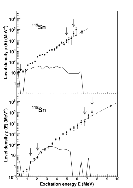
Figure 1: Normalized level densities of ¹¹⁹Sn (upper panel) and ¹¹⁸Sn (lower panel) as a function of excitation energy. Our experimental data are marked with filled squares. The dashed lines are the BSFG predictions that are used for interpolation, scaled to coincide with $\rho(S_{n})$ (open squares), which are calculated from neutron resonance data. The solid lines represent the discrete level densities obtained from counting the known levels. The arrows indicate the regions used to normalize the absolute values and the slope. The energy bins are 360 and 240 keV/ch for ^118,119Sn, respectively.

Figure 1 shows the normalized level densities in ^118,119Sn. The arrows indicate the regions used for normalization. As expected, the level densities of ¹¹⁹Sn and ¹¹⁸Sn are very similar to those of ¹¹⁷Sn and ¹¹⁶Sn Sn_Density , respectively.

The figure also shows that the known discrete levels ToI seem to be complete up to $\sim$ 2 MeV in ¹¹⁹Sn and up to $\sim 3$ MeV in ¹¹⁸Sn. Hence, our experiment has filled a region of unknown level density from the discrete region and to the gap, approximately at $\left(S_{n}-1\right)$ MeV. Unlike ¹¹⁹Sn, the ground-state of the even-even nucleus ¹¹⁸Sn has no unpaired neutron, and accordingly it has fewer available states than ¹¹⁹Sn. Therefore, measuring all levels to higher excitation energies by conventional methods is easier in ¹¹⁸Sn.

An alternative interpolation method to describe the gap between our measured data and the neutron resonance data based $\rho(S_{n})$ is the constant temperature (CT) model Gil65 . This approximation gives

$$\rho(E)=\frac{1}{T}\exp\left[\left(E-E_{0}\right)/T\right]\,,$$ (10)

where the "temperature" $T$ and the energy shift $E_{0}$ are treated as free parameters. Figure 2 shows a comparison of the CT model and the BSFG model as interpolation methods for ¹¹⁸Sn. The small difference in the region of interpolation is negligible for the normalization procedure.

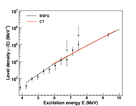
Figure 2: (Color online.) Comparison of the BSFG model (dashed line) and the CT model (solid line) as interpolation means for the level density of ¹¹⁸Sn. The arrows indicate the region of normalization. The parameters in the CT model ($T=0.86$ MeV and $E_{0}=-1.7$ MeV) have been found from a least $\chi^{2}$ fit to the data points in this region and from matching $\rho(S_{n})$, and the parameterization is not intended to be appropriate elsewhere.

III.2 Step-like structures

In Fig. 1, the level density of ¹¹⁹Sn shows a step-like structure superimposed on the general level density, which is smoothly increasing as a function of excitation energy. A step is characterized by an abrupt increase of level density within a small energy interval. The phenomenon of steps was also seen in ^116,117Sn Sn_Density .

Distinctive steps in ¹¹⁹Sn are seen below $\sim 4$ MeV. They are, together with the steps of ^116,117Sn Sn_Density , the most distinctive steps measured so far at OCL. This may be explained by Sn having a magic number of protons, $Z=50$. As long as the excitation energy is less than the energy of the proton shell gap, only neutron pairs are broken. The steps are distinctive since no proton pair-breaking smears the level density function.

The steps are less pronounced for ¹¹⁸Sn than for ¹¹⁹Sn. This is in contradiction to what is expected, as ¹¹⁸Sn is an even-even nucleus without the unpaired neutron reducing the clearness of the steps in ¹¹⁹Sn. The explanation probably lies in poorer statistics for the $(^{3}{\rm He},\alpha)$ reaction channel than for $(^{3}{\rm He},^{3}{\rm He}^{\prime})$. To reduce the error bars, a larger energy bin is chosen for ¹¹⁸Sn, leading to smearing the data and less clear structures.

Two steps in ¹¹⁹Sn are particularly distinctive: one at $\sim~{}1.0$ MeV and another at $\sim~{}2.0$ MeV, leading to bumps in the region around $\sim(1.2-1.4)$ MeV and around $\sim(2.2-2.6)$ MeV, respectively. The steps in ¹¹⁹Sn are found at approximately the same locations as in ¹¹⁷Sn Sn_Density .

Also for ¹¹⁶Sn, two steps were clearly seen for low excitation energy Sn_Density . The first of these is probably connected to the isotope’s first excited state, at 1.29 MeV ToI . A similar step in ¹¹⁸Sn would probably also had been found connected to the first excited state, at 1.23 MeV ToI , if the measured data had had better statistics.

Microscopic calculations based on the seniority model indicate that step structures in level density functions may be explained by the consecutive breaking of nucleon Cooper pairs Fe+Mo_lev . The steps for ¹¹⁹Sn in Fig. 1 are probable candidates for the neutron pair-breaking process. The neutron pair-breaking energy of ¹¹⁹Sn is estimated to be $2\Delta_{\rm n}=2.5$ MeV, which supports neutron pair-breaking as the origin of the pronounced bump around $\sim(2.2-2.6)$ MeV.

However, if the applied values of the neutron pair-gap parameters are accurate, the pronounced step at $\sim 1.0$ MeV in ¹¹⁹Sn and other steps below this energy are probably not due to pure neutron pair-breaking. They might be due to more complex structures, involving collective effects such as vibrations and/or rotations. In Sec. IV.3, the pair-breaking in our isotopes will be investigated further.

III.3 Entropy

In many fields of natural science, the entropy is used to reveal the degree of order/disorder of a system. In nuclear physics, the entropy may describe the number of ways the nucleus can arrange for a certain excitation energy. Various thermodynamic quantities may be deduced from the entropy, e.g., temperature, heat capacity and chemical potential. The study of nuclear entropy also exhibits the amount of entropy gained from the breaking of Cooper pairs. We would like to study the entropy difference between odd-$A$ and even-even Sn isotopes.

The microcanonical entropy is defined as

$$S_{s}(E)=k_{\rm B}\ln\Omega_{s}(E)\,,$$ (11)

where $k_{\rm B}$ is the Boltzmann constant, which is set to unity to make the entropy dimensionless, and where $\Omega_{s}(E)$ is the state density (multiplicity of accessible states). The state density is proportional to the experimental level density $\rho(E)$ by

$$\Omega_{s}(E)\propto\rho(E)\cdot\left[2\left<I(E)\right>+1\right]\,,$$ (12)

where $\left<I(E)\right>$ is the average spin within an energy bin of excitation energy $E$. The factor $2\left<I(E)\right>+1$ is the spin degeneracy of magnetic substates.

The spin distribution is not well-known, so we assume the spin degeneracy factor to be constant and omit it. Omitting this factor is firstly grounded by the spin being averaged over each energy bin, leading to only the absolute value of the state density at high excitation energies being altered, and not the structure. Secondly, the average spin $\left<I(E)\right>$ is expected to be a slowly varying function of energy (see Sec. IV). Hence, a "pseudo" entropy $S_{l}$ may be defined based only on the level density $\rho(E)$:

$$S_{l}\left(E\right)=k_{\rm B}\ln\left(\frac{\rho(E)}{\rho_{0}}\right)\,.$$ (13)

The constant $\rho_{0}$ is chosen so that $S_{l}=0$ in the ground state of the even-even nucleus ¹¹⁸Sn. This is satisfied for $\rho_{0}=0.135$ MeV^-1. The same value of $\rho_{0}$ is used for ¹¹⁹Sn.

Figure 3 shows the experimental results for the pseudo entropies of ^118,119Sn. These pseudo entropy functions are very similar to those of ^116,117Sn Sn_Density , which is as expected from the general similarity of the level density functions of these isotopes.

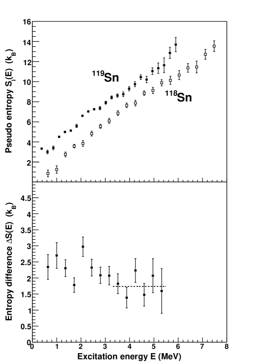
Figure 3: Upper panel: Experimental pseudo entropies $S_{l}$ of ¹¹⁹Sn (filled squares) and ¹¹⁸Sn (open squares) as a function of excitation energy. Lower panel: The respective experimental entropy difference, $\Delta S={S_{l}}^{119}-{S_{l}}^{118}$, as a function of excitation energy. An average value of $\overline{\Delta S}(E)=\left(1.7\pm 0.2\right)k_{B}$ is obtained from a $\chi^{2}$-fit (dashed line) to the experimental data above $\sim 3$ MeV.

We define the entropy difference as

$$\Delta S(E)={S_{l}}^{A}-{S_{l}}^{A-1}\,,$$ (14)

where the superscript denotes the mass number of the isotope. Assuming that entropy is an extensive quantity, the entropy difference will be equal to the entropy of the valence neutron, i.e. the experimental single neutron entropy of ^ASn.

For midshell nuclei in the rare-earth region, a semi-empirical study gutt4 has shown that the average single nucleon entropy is $\overline{\Delta S}\simeq 1.7~{}k_{B}$. This is true for a wide range of excitation energies, e.g., both for 1 and 7 MeV. Hence for these nuclei, the entropy simply scales with the number of nucleons not coupled in Cooper pairs, and the entropy difference is merely a simple shift with origin from the pairing energy.

Figure 3 also shows the entropy difference $\Delta S$ of ^118,119Sn, which are midshell in the neutrons only. Above $\sim 3$ MeV, the entropy difference may seem to approach a constant value. In the energy region where the entropy difference might be constant (shown as the dashed line in Fig. 3), we have calculated its mean value as $\overline{\Delta S}=\left(1.7\pm 0.2\right)k_{B}$. Within the uncertainty, this limit is in good agreement with the general conclusion of the above mentioned semi-empirical study gutt4 , and with the findings for ^116,117Sn Sn_Density . For lower excitation energy, however, Fig. 3 shows that the entropy difference of ^118,119Sn is not a constant, unlike the rare-earth midshell nuclei. Hence, the ^118,119Sn isotopes have an entropy difference that is more complicated than a simple excitation energy shift of the level density functions.

IV Nuclear properties extracted with a combinatorial BCS model

A simple microscopic model CecSc ; SyedTi ; MagneProceedings has been developed for further investigation of the underlying nuclear structure resulting in the measured level density functions. The model distributes Bardeen-Cooper-Schrieffer (BCS) quasi-particles on single-particle orbitals to make all possible proton and neutron configurations for a given excitation energy $E$. On each configuration, collective energy terms from rotation and vibration are schematically added. Even though this is a very simple representation of the physical phenomena, this combinatorial BCS model reproduces rather well the experimental level densities. As a consequence, the model is therefore assumed to be able to predict also other nuclear properties of the system. We are first and foremost interested in investigating the level density steps, and in investigating the assumption of parity symmetry, used in the normalization processes of the Oslo method.

IV.1 The model

The single-particle energies $e_{\rm sp}$ are calculated from the Nilsson model for a nucleus with an axially deformed core of quadrupole deformation parameter $\epsilon_{2}$. The values of the deformation parameters are $\epsilon_{2}=0.111$ and $\epsilon_{2}=0.109$ RIPL-2 for ^118,119Sn, respectively. Also needed for the calculation of the Nilsson energy scheme are the Nilsson parameters $\kappa$ and $\mu$ and the oscillator quantum energy between the main oscillator shells: $\hbar\omega_{0}=41A^{-1/3}$. The adopted values are $\kappa=0.070$ and $\mu=0.48$ for both neutrons and protons and for both nuclei, in agreement with the suggestion of Ref. KappaMy . All input parameters are listed in Tab. 2. The resulting Nilsson scheme for ¹¹⁸Sn is shown in Fig. 4.

Table 2: Input parameters used in the combinatorial BCS model, and the resulting values for the Fermi levels $\lambda_{\nu}$ (neutrons) and $\lambda_{\pi}$ (protons).

Nucleus	$\epsilon_{2}$	$\kappa$	$\mu$	$\hbar\omega_{0}$	$A_{\mathrm{gs}}$	$A_{\mathrm{rigid}}$	$\hbar\omega_{\mathrm{vib,\,e-e}}$	$\lambda_{\nu}$	$\lambda_{\pi}$
				(MeV)	(MeV)	(MeV)	(MeV)	(MeV)	(MeV)
119Sn	0.109	0.070	0.48	8.34	0.200	0.0122	1.23; 2.32	48.9	44.1
118Sn	0.111	0.070	0.48	8.36	0.205	0.0124	1.23; 2.32	48.9	44.2

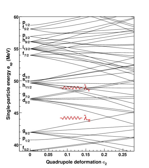
Figure 4: (Color online) The Nilsson level scheme, showing single-particle energies as functions of quadrupole deformation $\epsilon_{2}$, for ¹¹⁸Sn, which has $\epsilon_{2}=0.111$. The Nilsson parameters are set to $\kappa=0.070$ and $\mu=0.48$. The Fermi levels are illustrated as curled lines ($\lambda_{\pi}$ for protons, and $\lambda_{\nu}$ for neutrons).

The parameter $\lambda$ represents the quasi-particle Fermi level. It is iteratively determined by reproducing the right numbers of neutrons and protons in the system. The resulting Fermi levels for our nuclei are listed in Tab. 2 and illustrated for ¹¹⁸Sn in Fig. 4.

The microscopic model uses the concept of BCS quasi-particles BCS . Here, the single quasi-particle energies $e_{\rm qp}$ are defined by the transformation of:

$$e_{\rm qp}=\sqrt{\left(e_{\rm sp}-\lambda\right)^{2}+\Delta^{2}}\,.$$ (15)

The pair-gap parameter $\Delta$ is treated as a constant, as before, and with the same values.

The proton and neutron quasi-particle orbitals are characterized by their spin projections on the symmetry axes $\Omega_{\pi}$ and $\Omega_{\nu}$, respectively. The energy due to quasi-particle excitations is given by the sum of the proton and neutron energies and of a residual interaction $V$:

$$E_{\rm qp}(\Omega_{\pi},\Omega_{\nu})=\sum_{\{\Omega^{\prime}_{\pi},\,\Omega^{\prime}_{\nu}\}}e_{\rm qp}(\Omega_{\pi}^{\prime})+e_{\rm qp}(\Omega_{\nu}^{\prime})+V(\Omega_{\pi}^{\prime},\Omega^{\prime}_{\nu})\,.$$ (16)

In the model, quasi-particles having $\Omega$’s of different sign will have the same energy, i.e. one has a level degeneracy. Since no such degeneracy is expected, a Gaussian random distribution $V$ is introduced to compensate for a residual interaction apparently not taken into account by the Hamiltonian of the model. The maximum allowed number of broken Cooper pairs in our system is 3, giving a total of 7 quasi-particles for the even-odd nucleus ¹¹⁹Sn. Technically, all configurations are found from systematic combinations.

On each configuration, both a vibrational band and rotations are built. The energy of each level is found by adding the energy of the configuration and the vibrational and rotational terms:

$$E=E_{\rm qp}(\Omega_{\pi},\Omega_{\nu})+\hbar\omega_{\rm vib}\nu+A_{\rm rot}R\left(R+1\right)\,.$$ (17)

The vibrational term is described by the oscillator quantum energy $\hbar\omega_{\rm vib}$ and the phonon quantum number $\nu=0,1,2,...$ The values of $\hbar\omega_{\rm vib}$ are found from the $2^{+}$ and $3^{-}$ vibrational states of the even-even nucleus and are shown in Tab. 2. The last term of Eq. (17) represents the rotational energy. The quantity $A_{\rm rot}=\hbar^{2}/2{\cal J}$ is the rotational parameter with ${\cal J}$ being the moment of inertia, and $R$ is the rotational quantum number. The rotational quantum number has the values of $R=0,1,2,3...$ for the even-odd nucleus of ¹¹⁹Sn, and $R=0,2,4...$ for the even-even nucleus of ¹¹⁸Sn.

For low excitation energy, the value of the rotational parameter $A_{\rm rot}$ is determined around the ground state $A_{\rm gs}$. At high energy, the rotation parameter is found from a rigid, elliptical body, which is Krane :

$$A_{\rm rigid}=\frac{5\hbar^{2}}{4MR^{2}_{A}\left(1+0.31\epsilon_{2}\right)}\,.$$ (18)

Here, $M$ is the mass and $R_{A}$ the radius of the nucleus. For nuclei in the medium mass region, $A\sim 50-70$, the rotational parameter $A_{\rm rigid}$ is obtained at the neutron separation energy, according to a theoretical prediction Alhassid . We assume that $A_{\rm rigid}$ is obtained at the neutron separation energy also for our nuclei. The applied values of $A_{\rm gs}$ and $A_{\rm rigid}$ are listed in Tab. 2. The function $A_{\rm rot}$ as a function of energy is estimated from a linear interpolation between these.

IV.2 Level density

In Fig. 5, the level density functions calculated by our model are compared with the experimental ones. We see that the model gives a very good representation of the level densities in the statistical area above 3 MeV for both isotopes. Not taking into account all collective bands known from literature, the model is not intended to reproduce the discrete level structure below the pair-breaking energy. The model also succeeds in reproducing the bump around $\sim(2.2-2.6)$ MeV for both isotopes, even though the onset of this bump in ¹¹⁹Sn appears to be slightly delayed. Above $\sim 2.6$ MeV, the step brings the level density to the same order of magnitude as the experimental values.

According to Eq. (8) and the relation between the intrinsic excitation energy $U$ and the pair-gap parameters $\Delta_{\rm p}$ and $\Delta_{\rm n}$ the log-scale slope of the level density function is dependent on the pair-gap parameters. Figure 5 shows that the model reproduces well the slopes of the level densities for both isotopes. This supports the applied values of the pair-gap parameters.

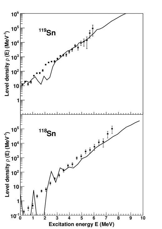
Figure 5: Level densities of ¹¹⁹Sn (upper panel) and ¹¹⁸Sn (lower panel) as a function of excitation energy. The solid lines are the theoretical predictions of the combinatorial BCS model. The squares are our experimental data.

IV.3 Pair-breaking

The pair breaking process produces a strong increase in the level density. Typically, a single nucleon entropy of $(1.6-1.7)\,k_{B}$ represents a factor of $\sim 5$ more levels due to the valence neutron. Thus, the breaking of a Cooper pair represents about 25 more levels. Pair-breaking is the most important mechanism for creating entropy in nuclei as function of excitation energy.

The average number of broken Cooper pairs per energy bin, $\left<N_{qp}\right>$, is calculated as a function of excitation energy by the model, using the adopted pair-gap parameters as input values. All configurations obtained for each energy bin are traced, and their respective numbers of broken pairs are counted. The average number of broken pairs is also calculated separately for proton and neutron pairs. The result for ^118,119Sn is shown in Fig. 6.

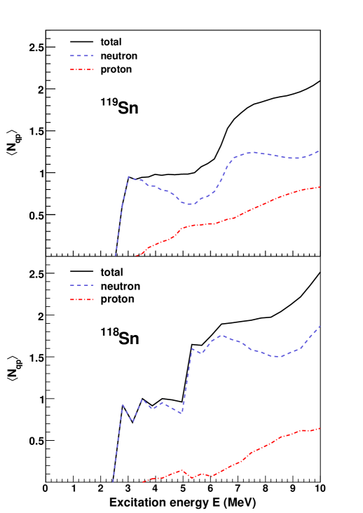
Figure 6: (Color online) The average number of broken quasi-particle pairs $\left<N_{qp}\right>$ (solid line) as a function of excitation enegy for ¹¹⁹Sn (upper panel) and ¹¹⁸Sn (lower panel), according to the combinatorial BCS model. Also shown is how this quantity breaks down into neutron pairs (dashed line) and proton pairs (dashed-dotted line).

Figure 6 shows that the first pair-breaking for both ^118,119Sn is at an excitation energy around $(2.2-2.6)$ MeV. That energy corresponds to the pair-breaking energy plus the extra energy needed to form the new configuration. The figure also shows that, according to the model, the pair-breakings here are only due to neutrons. The step in the average number of broken pairs is abrupt, and this number increases from 0 to almost 1. This means that there is a very high probability for the nucleus to undergo a neutron pair-breaking at this energy. Provided that our values of the pair-gap parameters are reasonable, so that this intense step in the number of broken neutron pairs in the model corresponds to the distinctive step in level density at $\sim 2.0$ MeV in ¹¹⁹Sn (see Sec. III), that step in level density is probably purely due to neutron pair-breaking.

The increases in the average number of broken pairs are abrupt also for certain other excitation energies, namely around $(5-6)$ MeV and $(8-9)$ MeV, as shown in Fig. 6. Here, we predict increases of the numbers of levels, caused by pair-breaking, even though not necessarily visible with the applied experimental resolution. In between the abrupt pair-breakings, the number of broken pairs is almost constant and close to integers. Saturation has been reached, and significantly more energy is needed for the next pair-breaking.

Neutron pair-breaking dominates over proton pair-breaking for the energies studied. Even though there is a large shell gap for the protons, breaking of proton pairs also occurs, but then only for energies above the proton pair-breaking energy of $2\Delta_{\rm p}$ plus the shell gap energy. According to Fig. 6, proton pair-breaking contributes for excitation energies above 3.5 MeV in both isotopes. An increased number of broken proton pairs at higher energies is expected to lead to the level density steps at high excitation energy being smeared out and becoming less distinctive, in accordance with the experimental findings of Sec. III.2.

Two effects due to the Pauli principle are notable in Fig. 6. In ¹¹⁹Sn compared to ¹¹⁸Sn, 1) the increases of the total average number of broken pairs occur at higher energies; and 2) the average number of broken proton pairs is generally higher. The explanation probably is that the valence neutron in ¹¹⁹Sn to some extent hinders the neutron pair-breaking. The presence of the valence neutron makes fewer states available for other neutrons, due to the Pauli principle. Therefore, in ¹¹⁹Sn compared to ¹¹⁸Sn, more energy is needed to break neutron pairs, and for a certain energy, proton pair-breaking is more probable. Of course, an increase in the number of broken proton pairs leads to a corresponding decrease in the number of broken neutron pairs.

IV.4 Collective effects

We have made use of the model to make a simple estimate of the relative impact on the level density of collective effects, i.e., rotations and vibrations, compared to that of the pair-breaking process. The enhancement factor of the collective effects is defined as

$$F_{\rm coll}(E)=\frac{\rho(E)}{\rho_{\rm non-coll}(E)}\,,$$ (19)

where $\rho_{\rm non-coll}$ is the level density function excluding collective effects.

Figure 7 shows the calculated level density with and without collective contributions from vibrations and from rotational bands for ¹¹⁹Sn. The model prediction is assumed to be reasonably valid above $\sim 3$ MeV of excitation energy. According to these simplistic calculations, the enhancement factor of collective effects $F$ sharply decreases at the energies of the steps in the average number of broken quasi-particle pairs (see Fig. 6). For ¹¹⁹Sn, we find that $F$ decreases for excitation energies of approximately 2.5 and 6 MeV, where the average number of broken quasi-particle pairs increase from $\sim 0$ to $\sim 1$, and from $\sim 1$ to $\sim 2$, respectively. For the energies studied, the maximum value of $F$ is about 10, found at $E\simeq 6$ MeV. For ¹¹⁸Sn, the enhancement factor would be less than for ¹¹⁹Sn, since this nucleus does not have unpaired valence neutrons.

As a conclusion, the collective phenomena of vibrations and rotations seem to have a significantly smaller impact on the creation of new levels than the nucleon pair-breaking process, which has an enhancement factor of typically about 25 for each broken pair.

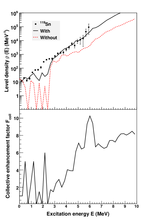
Figure 7: (Color online) The impact of collective effects on the level density of ¹¹⁹Sn according to the combinatorial BCS model. The upper panel shows experimental level density (data points) compared with model calculations with collective effects (solid line) and without collective effects (dashed line). The lower panel shows the corresponding enhancement factor of the collective effects, $F_{\rm coll}$ (linear scale).

IV.5 Parity asymmetry

The parity asymmetry function $\alpha$ is defined as

$$\alpha=\frac{\rho_{+}-\rho_{-}}{\rho_{+}+\rho_{-}}\,,$$ (20)

where $\rho_{+}$ is the level density of positive parity states, and $\rho_{-}$ is the level density of the negative parity states. The values of $\alpha$ range from $-1$ to $+1$. A system with $\alpha=-1$ is obtained for $\rho_{+}=0$, implying that all states have a negative parity. A system with $\alpha=0$ has equally many states with positive as negative parity and is obtained for $\rho_{-}=\rho_{+}$.

The Nilsson scheme in Fig. 4 shows that the single-particle orbitals both above and below the neutron Fermi level are a mixture of positive and negative parities. In addition, each of these states may be the head of vibrational bands, for which the parity of the band may be opposite of that of the band head.

The parity asymmetry functions of ^118,119Sn are drawn in Fig. 8. For energies below the neutron pair-breaking energy approximately at 2.5 MeV, the even-odd isotope has a parity asymmetry function with large fluctuations between positive and negative values, while the even-even isotope has positive parities. This is as expected when vibrational bands of opposite parity are not introduced. (The zero parity of ¹¹⁸Sn for certain low-energy regions is explained by the non-existence of energy levels.)

Above the pair-breaking energies, the asymmetry functions begin to approach zero for both isotopes. This is also as expected, since we then have a group of valence nucleons that will randomly occupy orbitals of positive and negative parity and on average give an $\alpha$ close to zero. Above $\sim 4$ MeV, the parity distributions of ^118,119Sn are symmetric with $\rho_{+}\simeq\rho_{-}$. This is a gratifying property, since parity symmetry is an assumption in the Oslo method normalization procedure for both the level density and the $\gamma$-ray strength function (see Sec. V).

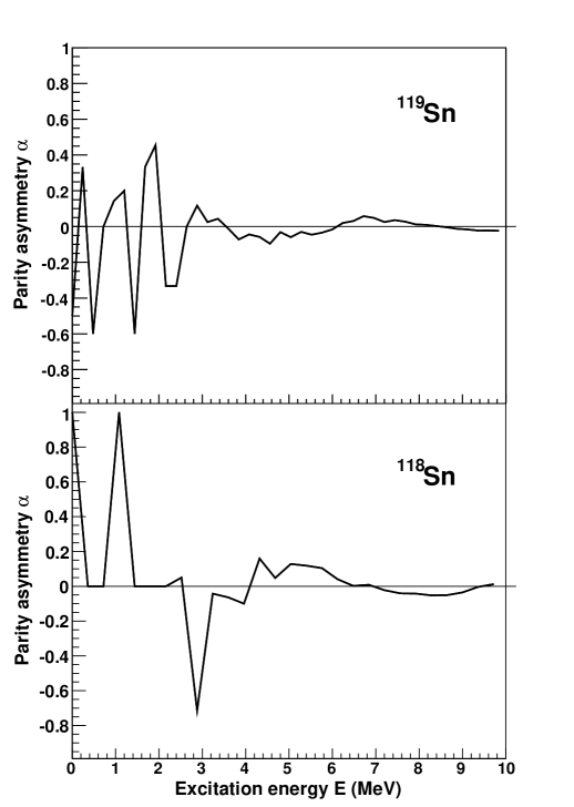
Figure 8: The parity asymmetry function $\alpha$, according to the combinatorial BCS model, shown as a function of excitation energy for ¹¹⁹Sn (upper panel) and ¹¹⁸Sn (lower panel).

IV.6 Spin distribution

The combinatorial BCS model determines the total spin $I$ for each level from the relation:

$$I\left(I+1\right)=R\left(R+1\right)+\sum_{\Omega_{\pi},\,\Omega_{\nu}}\Omega_{\pi}+\Omega_{\nu}\,,$$ (21)

from which the spin distribution of the level density $\rho$ may be estimated.

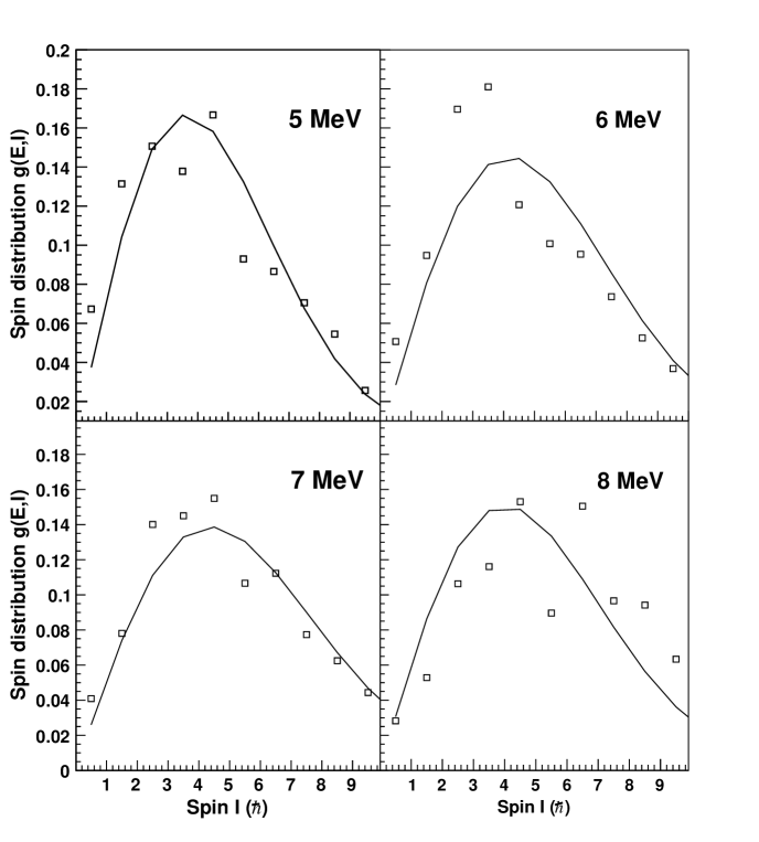
Figure 9: Comparison of spin distributions in ¹¹⁸Sn at different excitation energies. The open squares are calculated from the combinatorial BCS model in Eq. (21), while the solid lines are the predictions of Gilbert and Cameron in Eq. (4). The spin distributions are normalized to 1.

The resulting spin distribution is compared with the theoretical spin distribution of Gilbert and Cameron in Eq. (4), using the same parameterization of the spin cutoff parameter as Eq. (5). Figure 9 shows the comparison for four different excitation energies: 5, 6, 7 and 8 MeV. The agreement is generally good. Hence, the spin calculation in Eq. (21), and the assumption of the rigid rotational parameter $A_{\rm rigid}$ obtained at $S_{n}$, are indicated to be reasonable assumptions. We also note from the figure that the average spin, $\left<I(E)\right>$, is only slowly increasing with excitation energy, justifying the pseudo entropy definition introduced in Eq. (13).

V Gamma-ray strength functions

V.1 Normalization and experimental results

The $\gamma$-ray transmission coefficient ${\cal T}$, which is deduced from the experimental data, is related to the $\gamma$-ray strength function $f$ by

$${\cal T}(E_{\gamma})=2\pi\sum_{XL}E_{\gamma}^{2L+1}f_{XL}(E_{\gamma})\,,$$ (22)

where $X$ denotes the electromagnetic character and $L$ the multipolariy of the $\gamma$-ray. The transmission coefficient ${\cal T}$ is normalized in slope $\alpha$ and in absolute value $B$ according to Eq. (3). The slope was determined in Sec. III in the case of ^118,119Sn, and in Ref. Sn_Density in the case of ¹¹⁶Sn. The absolute value normalization is yet to be determined. This is done using the literature values of the average total radiative width at the neutron separation energy, $\left<\Gamma_{\gamma}(S_{n})\right>$, which are measured for neutron capture reactions $(n,\gamma)$.

The $\gamma$-ray transmission coefficient ${\cal T}$ is related to the average total radiative width $\left<\Gamma_{\gamma}(E,I,\pi)\right>$ of levels with energy $E$, spin $I$ and parity $\pi$ by Kopecky :

$$\left<\Gamma_{\gamma}(E,I,\pi)\right>=\frac{1}{2\pi\,\rho(E,I,\pi)}$$ (23)

$$\times\sum_{XL}\sum_{I_{f},\,\pi_{f}}\int_{E_{\gamma}}^{E}{\rm d}E_{\gamma}{\cal T}_{XL}(E_{\gamma})\,\rho(E-E_{\gamma},I_{f},\pi_{f})\,.$$

The summations and integration are over all final levels of spin $I_{f}$ and parity $\pi_{f}$ that are accessible through a $\gamma$-ray transition categorized by the energy $E_{\gamma}$, electromagnetic character $X$ and multipolarity $L$.

For $s$-wave neutron resonances and assuming a major contribution from dipole radiation and parity symmetry for all excitation energies, the general expression in Eq. (23) will at $S_{n}$ reduce to

$$\left<\Gamma_{\gamma}(S_{n},I_{t}\pm 1/2,\pi_{t})\right>$$ (24)

$$= \frac{B}{4\pi\,\rho(S_{n},I_{t}\pm 1/2,\pi_{t})}\int_{0}^{S_{n}}{\rm d}E_{\gamma}\,{\cal T}(E_{\gamma})\,\rho(S_{n}-E_{\gamma})$$

$$\times\sum_{J=-1}^{1}g(S_{n}-E_{\gamma},I_{t}\pm 1/2+J)\,.$$

Here, $I_{t}$ and $\pi_{t}$ are the spin and parity of the target nucleus in the $(n,\gamma)$ reaction. Indeed, the results from the combinatorial BCS model in Sec. IV supports the symmetry assumption of the parity distribution. The normalization constant $B$ in Eq. (24) is determined Voinov01 by replacing ${\cal T}$ with the experimental transmission coefficient, $\rho$ with the experimental level density, $g$ with the spin distribution given in Eq. (4), and $\left<\Gamma_{\gamma}(S_{n})\right>$ with its literature value.

The input parameters needed for determining the normalization constant $B$ for ^118,119Sn are shown in Tab. 3 and taken from Ref. RIPL-3 . For ¹¹⁶Sn, the level spacing $D_{0}(S_{n})$ is not available in the literature. Therefore, $\rho(S_{n})$ was estimated from systematics for the normalization of $\alpha$ in Ref. Sn_Density . The value of $D_{0}$ in Tab. 3 is estimated from $\rho(S_{n})$. Note that there was an error in the spin cutoff parameters $\sigma(S_{n})$ of ^116,117Sn in Refs. Sn_Density ; Sn_Strength . The impact of this correction on the normalization of level densities and strength functions is very small. Moreover, updated values of $D_{0}(S_{n})$ and $\left<\Gamma_{\gamma}(S_{n})\right>$ are now available for ¹¹⁷Sn RIPL-3 . All the new normalization parameters for ^116,117Sn are presented in Tab. 4. The value of $\left<\Gamma_{\gamma}(S_{n})\right>$ of ¹¹⁶Sn is taken from the indicated value in Ref. RIPL-3 .

Table 3: Input parameters for normalization of the $\gamma$-ray transmission coefficient ${\cal T}$ for ^118,119Sn.

Nucleus	$I_{t}$	$D_{0}(S_{n})$	$\left<\Gamma_{\gamma}(S_{n})\right>$
	($\hbar$)	(eV)	(meV)
119Sn	0	700	45
118Sn	1/2	61	117

Table 4: New normalization parameters for ^116,117Sn.

Nucleus	$\sigma(S_{n})$	$D_{0}(S_{n})$	$\rho(S_{n})$	$\left<\Gamma_{\gamma}(S_{n})\right>$	$\eta$
		(eV)	($10^{4}$ MeV-1)	(meV)
117Sn	4.58	450(50)	9.09(2.68)	52	0.43
116Sn	4.76	59	40(20)	120	0.45

The resulting $\gamma$-ray strength functions of ^116-119Sn are shown in Fig. 10. For all isotopes, it is clear that there is a change of the log-scale derivate at $E_{\gamma}\sim 4$ MeV, leading to a sudden increase of strength. Such an increase may indicate the onset of a resonance. The comparison in Fig. 10 of the new ¹¹⁷Sn strength function with the earlier published one Sn_Strength confirms that correcting the $\sigma(S_{n})$ and the $D_{0}(S_{n})$ had only a minor impact on the normalization.

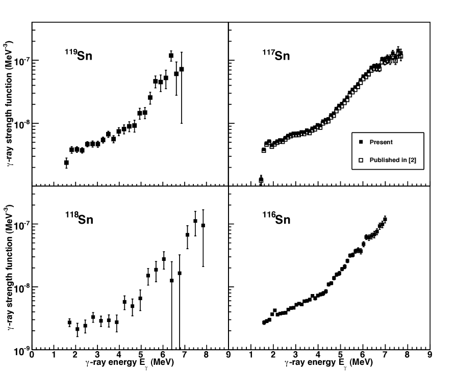
Figure 10: Normalized $\gamma$-ray strength functions as functions of $\gamma$-ray energy. The upper panels show ¹¹⁹Sn (left) and both present and previously published versions of ¹¹⁷Sn (right). The energy bins 120 and 240 keV/ch for ^117,119Sn, respectively. The lower panels show ¹¹⁸Sn (left) and ¹¹⁶Sn (right) with the energy bins of 360 and 120 keV/ch, respectively.

Figure 11 shows the four normalized strength functions of ^116-119Sn together. They are all approximately equal except for ¹¹⁸Sn, which has a lower absolute normalization than the others. This is surprising considering the quadrupole deformation parameter of ¹¹⁸Sn ($\varepsilon_{2}=0.111$) being almost identical to that of ¹¹⁶Sn ($\varepsilon_{2}=0.112$) RIPL-2 . In the following, we therefore multiply the strength of ¹¹⁸Sn with a factor of 1.8 to get it on the same footing as the others. The values of $\rho(S_{n})$ and the scaling parameter $\eta$ (see also Sec. III.1) of these Sn isotopes are collected in Tab. 5. For ¹¹⁸Sn, the $\rho(S_{n})$ may be expected to be larger, while $\eta$ may be expected to be smaller. It would be desirable to remeasure both $D_{0}(S_{n})$ and $\left<\Gamma_{\gamma}\right>$ for this isotope, since the apparent wrong normalization of the strength function of ¹¹⁸Sn depends on these parameters.

Table 5: The Fermigas approximation for $\rho(S_{n})_{\rm BSFG}$, the calculated $\rho(S_{n})$, and the resulting scaling parameter $\eta$, for ^116-119Sn.

Nucleus	$\rho(S_{n})_{\rm BSFG}$	$\rho(S_{n})$	$\eta$
	($10^{4}$ MeV-1)	($10^{4}$ MeV-1)
119Sn	14	6.05(175)	0.44
118Sn	65	38.4(86)	0.59
117Sn	22	9.09(2.68)	0.43
116Sn	89	40.0(20.0)	0.45

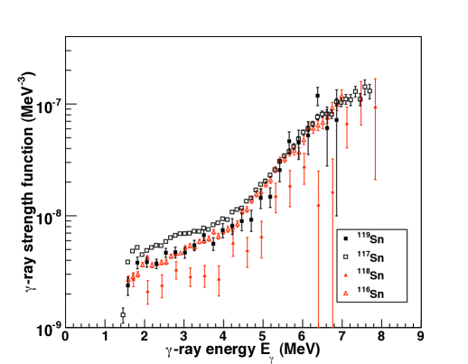
Figure 11: (Color online) The four normalized strength functions of ^116-119Sn shown together.

V.2 Pygmy resonance

Comparing our measurements with other experimental data makes potential resonances easier to localize. Experimental cross section data $\sigma(E_{\gamma})$ are converted to $\gamma$-ray strength $f(E_{\gamma})$ through the relation:

$$f(E_{\gamma})=\frac{1}{3\pi\hbar^{2}c^{2}}\left(\frac{\sigma(E_{\gamma})}{E_{\gamma}}\right)\,.$$ (25)

Figure 12 shows the comparison of the Oslo strength functions of ^116-119Sn with those of the photoneutron cross section reactions ${}^{116,117}{\rm Sn}(\gamma,n)$ from Utsunomiya et al. Utsunomiya and ${}^{119}{\rm Sn}(\gamma,n)$ from Varlamov et al. Varlamov09 , photoabsorption reactions ${}^{116-119}{\rm Sn}(\gamma,x)$ from Fultz et al. Fultz69 , ${}^{116-118}{\rm Sn}(\gamma,x)$ from Varlamov et al. Varlamov03 , and ${}^{116-118}{\rm Sn}(\gamma,x)$ from Leprêtre et al. Lepretre74 . Clearly, the measurements on ^117,119Sn both from Oslo and from Utsunomiya et al. Utsunomiya independently indicate a resonance, from the changes of slopes. For ^116,118Sn, the Oslo data clearly shows the presence of resonances. Hence, the resonance earlier observed in ¹¹⁷Sn Sn_Strength is confirmed also in ^116,118,119Sn. This resonance will be referred to as the pygmy resonance.

In order to investigate the experimental strength functions further, and in particular the pygmies, we have applied commonly used models for the Giant Electric Dipole Resonance (GEDR) and for the magnetic spin-flip resonance, also known as the Giant Magnetic Dipole Resonance (GMDR).

For the GEDR resonance, the Generalized Lorentzian (GLO) model Kopecky87 is used. The GLO model is known to agree well both for low $\gamma$-ray energies, where we measure, and for the GEDR centroid at about 16 MeV. The strength function approaching a non-zero value for low $E_{\gamma}$ is not a property specific for the Sn isotopes, but has been the case for all nuclei studied at the OCL so far.

In the GLO model, the $E1$ strength function is given by Kopecky87 :

$$f^{\rm GLO}_{E1}(E_{\gamma}) = \frac{1}{3\pi^{2}\hbar^{2}c^{2}}\sigma_{E1}\,\Gamma_{E1}$$

$$\times \left[E_{\gamma}\,\frac{\Gamma_{KMF}(E_{\gamma},T_{f})}{\left({E_{\gamma}}^{2}-{E_{E1}}^{2}\right)^{2}+{E_{\gamma}}^{2}\left(\Gamma_{KMF}(E_{\gamma},T_{f})\right)^{2}}\right.$$

$$+ \left.0.7\,\frac{\Gamma_{KMF}(E_{\gamma}=0,T_{f})}{{E_{E1}}^{3}}\right]$$

in units of ${\rm MeV}^{-3}$, where the Lorentzian parameters are the GEDR’s centroid energy $E_{E1}$, width $\Gamma_{E1}$ and cross section $\sigma_{E1}.$ We use the experimental parameters of Fultz Fultz69 , shown in Tab. 6. The GLO model is temperature dependent from the incorporation of a temperature dependent width $\Gamma_{KMF}$. This width is the term responsible for ensuring the non-vanishing GEDR at low excitation energy. It has been adopted from the Kadmenskiĭ, Markushev and Furman (KMF) model KMF and is given by:

$$\Gamma_{KMF}(E_{\gamma},T_{f})=\frac{\Gamma_{r}}{{E_{r}}^{2}}\left({E_{\gamma}}^{2}+4\pi^{2}{T_{f}}^{2}\right)\,,$$ (27)

in units of MeV.

Usually, $T_{f}$ is interpreted as the nuclear temperature of the final state, with the commonly applied expression $T_{f}=~{}\sqrt{U/a}$. On the other hand, we are assuming a constant temperature, i.e., the $\gamma$-ray strength function is independent of excitation energy. This approach is adopted for consistency with the Brink-Axel hypothesis (see Sec. II), where the strength function was assumed to be temperature independent. Moreover, we treat $T_{f}$ as a free parameter in order to fit in the best possible way the theoretical strength prediction to the low energy measurements. The applied values of $T_{f}$ are listed in Tab. 6.

Table 6: Parameters used for the theoretical $\gamma$-ray strength functions of ^116-119Sn. The value of $T_{f}$ in ¹¹⁸Sn has been found for the measured strength function multiplied by 1.8.

Nucleus	$E_{E1}$	$\Gamma_{E1}$	$\sigma_{E1}$	$E_{M1}$	$\Gamma_{M1}$	$\sigma_{M1}$	$T_{f}$
	(MeV)	(MeV)	(mb)	(MeV)	(MeV)	(mb)	(MeV)
119Sn	15.53	4.81	253.0	8.34	4.00	0.963	0.40(1)
118Sn	15.59	4.77	256.0	8.36	4.00	0.956	0.40(1)
117Sn	15.66	5.02	254.0	8.38	4.00	1.04	0.46(1)
116Sn	15.68	4.19	266.0	8.41	4.00	0.773	0.46(1)

The $M1$ spin-flip resonance is modeled with the functional form of a Standard Lorentzian (SLO) RIPL-2 :

$$f_{M1}^{\rm SLO}(E_{\gamma})=\frac{1}{3\pi^{2}\hbar^{2}c^{2}}\frac{\sigma_{M1}{{\Gamma}_{M1}}^{2}E_{\gamma}}{\left({E_{\gamma}}^{2}-{E_{M1}}^{2}\right)^{2}+{E_{\gamma}}^{2}\,{\Gamma_{M1}}^{2}}\,,$$ (28)

where the parameter $E_{M1}$ is the centroid energy, $\Gamma_{M1}$ the width and $\sigma_{M1}$ the cross section, of the GMDR. These Lorentzian parameters are predicted from the expressions in Ref. RIPL-2 , with the results as shown in Tab. 6.

In the absence of any established theoretical prediction about the pygmy resonance, we found that the pygmy is satisfactorily reproduced by a Gaussian distribution Sn_Strength :

$$f_{\rm pyg}(E_{\gamma})=C_{\rm pyg}\cdot\frac{1}{\sqrt{2\pi}\,\sigma_{\rm pyg}}\exp\left[\frac{-\left(E_{\gamma}-E_{\rm pyg}\right)^{2}}{2{\sigma_{\rm pyg}}^{2}}\right)\,,$$ (29)

where $C_{\rm pyg}$ is the pygmy’s normalization constant, $E_{\rm pyg}$ the energy centroid and $\sigma_{\rm pyg}$ the standard deviation. These parameters are treated as free. The total model prediction of the $\gamma$-ray strength function is then given by:

$$f_{\rm total}=f_{E1}+f_{M1}+f_{\rm pyg}\,.$$ (30)

By adjusting the Gaussian pygmy parameters to make the best fit to the experimental data of ^116-119Sn, we obtained the values as presented in Tab. 7. The pygmy fit of ¹¹⁷Sn is updated and corresponds to the present normalization of the strength function. The pygmy fit also gave an excellent fit for ¹¹⁶Sn. For ^118,119Sn, it was necessary to slightly reduce the values of $T_{f}$ and $\sigma_{\rm pyg}$. The similarity of the sets of parameters for the different nuclei is gratifying. As is seen in Fig. 12, these theoretical predictions describe the measurements rather well.

Figure 12: (Color online) Comparison of theoretical predictions including pygmy fits with experimental measurements for ^116-119Sn. The total strengths (solid lines) are modeled as Gaussian pygmy additions to the GLO (E1 + M1) baselines. The SLO (E1 + M1) baselines are also shown, failing to reproduce the measurements for low $E_{\gamma}$. The arrows indicate the neutron separation energies $S_{n}$.
Upper, left panel: Comparison of theoretical predictions of ¹¹⁹Sn with the Oslo measurements, ${}^{117}{\rm Sn}(\gamma,n)$ from Utsunomiya et al. Utsunomiya , ${}^{119}{\rm Sn}(\gamma,x)$ from Fultz et al. Fultz69 , and ${}^{119}{\rm Sn}(\gamma,n)$ from Varlamov et al. Varlamov09 .
Upper, right panel: Comparison of theoretical predictions of ¹¹⁷Sn with the Oslo measurements, ${}^{117}{\rm Sn}(\gamma,n)$ from Utsunomiya et al. Utsunomiya , ${}^{117}{\rm Sn}(\gamma,x)$ from Fultz et al. Fultz69 , ${}^{117}{\rm Sn}(\gamma,x)$ from Varlamov et al. Varlamov03 , and ${}^{117}{\rm Sn}(\gamma,x)$ from Leprêtre et al. Lepretre74 .
Lower, left panel: Comparison of theoretical predictions of ¹¹⁸Sn with the Oslo measurements multiplied with 1.8 (filled squares) (the measurements with the original normalization are also included as open squares), ${}^{116}{\rm Sn}(\gamma,n)$ from Utsunomiya et al. Utsunomiya , ${}^{118}{\rm Sn}(\gamma,x)$ from Fultz et al. Fultz69 , ${}^{118}{\rm Sn}(\gamma,x)$ from Varlamov et al. Varlamov03 , and ${}^{118}{\rm Sn}(\gamma,x)$ from Leprêtre et al. Lepretre74 .
Lower, right panel: Comparison of theoretical predictions of ¹¹⁶Sn with the Oslo measurements, ${}^{116}{\rm Sn}(\gamma,n)$ from Utsunomiya et al. Utsunomiya , ${}^{116}{\rm Sn}(\gamma,x)$ from Fultz et al. Fultz69 , ${}^{116}{\rm Sn}(\gamma,x)$ from Varlamov et al. Varlamov03 , and ${}^{116}{\rm Sn}(\gamma,x)$ from Leprêtre et al. Lepretre74 .

Table 7: Empirical values of ^116-119Sn pygmies Gaussian parameters, the integrated pygmy strengths and the TRK values. For ¹¹⁸Sn, the values have been found from fitting to the measured strength function multiplied by 1.8.

Nucleus	$C_{\rm pyg}$	$E_{\rm pyg}$	$\sigma_{\rm pyg}$	Int. strength	TRK value
	($10^{-7}{\rm MeV}^{-2})$	(MeV)	(MeV)	(MeV$\cdot$mb)	(%)
119Sn	3.2(3)	8.0(1)	1.2(1)	30(15)	1.7(9)
118Sn	3.2(3)	8.0(1)	1.2(1)	30(15)	1.7(9)
117Sn	3.2(3)	8.0(1)	1.4(1)	30(15)	1.7(9)
116Sn	3.2(3)	8.0(1)	1.4(1)	30(15)	1.7(9)

The pygmy centroids of all the isotopes are estimated to be around 8.0(1) MeV. It is noted that an earlier experiment by Winhold et al. Winhold using the $(\gamma,n)$ reactions determined the pygmy centroids for ^117,119Sn to approximately 7.8 MeV, in agreement with our measurements.

Extra strength has been added in the energy region of $\sim(4-11)$ MeV. The total integrated pygmy strengths are 30(15) MeV$\cdot$mb for all four isotopes. This constitutes $1.7(9)\%$ of the classical Thomas-Reiche-Kuhn (TRK) sum rule, assuming all pygmy strength being $E1$. Even though these resonances are rather small compared to the GEDR, they may have a non-negligible impact on nucleosynthesis in supernovas Goriely98 .

If one does not multiply the strength function of ¹¹⁸Sn by 1.8 for the footing equality, then the pygmy of ¹¹⁸Sn becomes very different from those of the other isotopes, and the total prediction is not able to follow as well the measurements for low $E_{\gamma}$. A pygmy fit of the original normalization does however give: $T_{f}=0.28(2)$ MeV, $C_{\rm pyg}=1.8(6)\cdot 10^{-7}{\rm MeV}^{-2}$, $E_{\rm pyg}=8.0(2)$ MeV and $\sigma_{\rm pyg}=1.0(1)$ MeV. This represents a smaller pygmy, giving an integrated strength of 17(8) MeV$\cdot$mb and a TRK value of $1.0(5)\%$.

The commonly applied Standard Lorentzian (SLO) was also tested as a model of the baseline and is included in Fig. 12. The SLO succeeds in reproducing the $(\gamma,x)$ data, but clearly fails for the low-energy strength measurements, both when it comes to absolute value and to shape. The same has been the case also for many other nuclei measured at the OCL. Therefore, we deem the SLO not to be adequate below the neutron threshold.

Probably, the pygmies of all the Sn isotopes are caused by the same phenomenon. It is still indefinite whether the Sn pygmy is of $E1$ or $M1$ character. A clarification would be of utmost importance.

Earlier studies indicate an $E1$ character of the Sn pygmy. Amongst these are the nuclear resonance fluorescence experiments (NRF) performed on ^116,124Sn Govaert and on ^112,124Sn Tonchev , and the Coulomb dissociation experiments performed on ^129-132Sn Adrich ; Klimkiewicz . If the Sn pygmy is of $E1$ character, it may be consistent with the so-called $E1$ neutron skin oscillation mode, discussed in Refs. Paar ; Sarchi ; Isacker .

However, the possibility of an $M1$ character cannot be ruled out. Figure 4 shows that the Sn isotopes have their proton Fermi level located right in between the $g_{7/2}$ and $g_{9/2}$ orbitals, and their neutron Fermi level between $h_{11/2}$ and $h_{9/2}$. Thus, an enhanced $M1$ resonance may be due to proton $g_{7/2}\leftrightarrow g_{9/2}$ and neutron $h_{11/2}\leftrightarrow h_{9/2}$ magnetic spin-flip transitions. The existence of an $M1$ resonance in this energy region has been indicated in an earlier experimental study: proton inelastic scattering experiment on ^120,124Sn Djalali .

VI Conclusions

The level densities of ^118,119Sn and the $\gamma$-ray strength functions of ^116,118,119Sn have been measured using the (³He,  $\alpha\gamma$) and (³He,³He${}^{\prime}\gamma$) reactions and the Oslo method.

The level density function of ¹¹⁹Sn shows pronounced steps for excitation energies below $\sim 4$ MeV. This may be explained by the fact that Sn has a closed proton shell, so that only neutron pairs are broken at low energy. Without any proton pair-breaking smearing out the level density function, the steps from neutron pair-breaking remain distinctive. The entropy has been deduced from the experimental level density functions, with a mean value of the single neutron entropy in ¹¹⁹Sn determined to $(1.7\pm 0.2)\,k_{B}$. These findings are in good agreement with those of ^116,117Sn.

A combinatorial BCS model has been used to extract nuclear properties from the experimental level density. The number of broken proton and neutron pairs as a function of excitation energy is deduced, showing that neutron pair-breaking is the most dominant pair-breaking process for the entire energy region studied. The enhancement factor of collective effects on level density contributes a maximum factor of about 10, which is small compared to that of pair-breaking. The parity distributions are found to be symmetric above $\sim 4$ MeV of excitation energy.

In all the ^116-119Sn strength functions, a significant enhancement is observed in the energy region of $E_{\gamma}\simeq(4-11)$ MeV. The integrated strength of the resonances correspond to $1.7(9)\%$ of the TRK sum rule. These findings are in agreement with the conclusions of earlier studies.

- (1) U. Agvaanluvsan, A. C. Larsen, M. Guttormsen, R. Chankova, G. E. Mitchell, A. Schiller, S. Siem, and A. Voinov, Phys. Rev. C 79, 014320 (2009).
- (2) U. Agvaanluvsan, A. C. Larsen, R. Chankova, M. Guttormsen, G. E. Mitchell, A. Schiller, S. Siem, and A. Voinov, Phys. Rev. Lett. 102, 162504 (2009).
- (3) M. Guttormsen, T. S. Tveter, L. Bergholt, F. Ingebretsen, and J. Rekstad, Nucl. Instrum. Methods Phys. Res. A 374, 371 (1996).
- (4) M. Guttormsen, T. Ramsøy, and J. Rekstad, Nucl. Instrum. Methods Phys. Res. A 255, 518 (1987).
- (5) A. Schiller, L. Bergholt, M. Guttormsen, E. Melby, J. Rekstad, and S. Siem, Nucl. Instrum. Methods Phys. Res. A 447, 498 (2000).
- (6) A. Bohr and B. Mottelson, Nuclear Structure (Benjamin, New York, 1969), Vol. I.
- (7) D. M. Brink, Ph.D. thesis, Oxford University, 1955.
- (8) P. Axel, Phys. Rev. 126, 671 (1962).
- (9) S. F. Mughabghab, Atlas of Neutron Resonances, Fifth Edition, Elsevier Science (2006).
- (10) R. Capote et al., RIPL-3 – Reference Input Parameter Library for Calculation of Nuclear Reactions and Nuclear Data Evaluations, Nuclear Data Sheets 110 (2009), 3107-3214. Available online at http://www-nds.iaea.org/RIPL-3/.
- (11) T. von Egidy, H. H. Schmidt, and A. N. Behkami, Nucl. Phys. A481, 189 (1988).
- (12) T. von Egidy and D. Bucurescu, Phys. Rev. C 72, 044311 (2005); 73, 049901(E) (2006).
- (13) H. Utsunomiya, S. Goriely, M. Kamata, T. Kondo, O. Itoh, H. Akimune, T. Yamagata, H. Toyokawa, Y.-W. Lui, S. Hilaire, and A. J. Koning, Phys. Rev. C 80, 055806 (2009).
- (14) A. Gilbert and A. G. W. Cameron, Can. J. Phys. 43, 1446 (1965).
- (15) G. Audi and A. H. Wapstra, Nucl. Phys. A595, 409 (1995).
- (16) J. Dobaczewski, P. Magierski, W. Nazarewicz, W. Satuła, and Z. Szymański, Phys. Rev. C 63, 024308 (2001).
- (17) N. U. H. Syed, M. Guttormsen, F. Ingebretsen, A. C. Larsen, T. Lönnroth, J. Rekstad, A. Schiller, S. Siem, and A. Voinov, Phys. Rev. C 79, 024316 (2009).
- (18) R. Firestone and V. S. Shirley, Table of Isotopes, 8th ed. (Wiley, New York, 1996), Vol. II.
- (19) A. Schiller, E. Algin, L. A. Bernstein, P. E. Garrett, M. Guttormsen, M. Hjorth-Jensen, C. W. Johnson, G. E. Mitchell, J. Rekstad, S. Siem, A. Voinov, and W. Younes, Phys. Rev. C 68, 054326 (2003).
- (20) M. Guttormsen, M. Hjorth-Jensen, E. Melby, J. Rekstad, A. Schiller, and S. Siem, Phys. Rev. C 63, 044301 (2001).
- (21) A. C. Larsen, M. Guttormsen, R. Chankova, F. Ingebretsen, T. Lönnroth, S. Messelt, J. Rekstad, A. Schiller, S. Siem, N. U. H.Syed, and A. Voinov, Phys. Rev. C 76, 044303 (2007).
- (22) N. U. H. Syed, A. C. Larsen, A. Bürger, M. Guttormsen, S. Harissopulos, M. Kmiecik, T. Konstantinopoulos, M. Krtička, A. Lagoyannis, T. Lönnroth, K. Mazurek, M. Norby, H. T. Nyhus, G. Perdikakis, S. Siem, and A. Spyrou, Phys. Rev. C 80, 044309 (2009).
- (23) M. Guttormsen, U. Agvaanluvsan, E. Algin, A. Bürger, A. C. Larsen, G. E. Mitchell, H. T. Nyhus, S. Siem, H. K. Toft, and A. Voinov, Properties of warm nuclei in the quasi-continuum, in Proceedings of the CNR* 09 Conference, to be published in EPJ Web of Conferences.
- (24) T. Belgya, O. Bersillon, R. Capote, T. Fukahori, G. Zhigang, S. Goriely, M. Herman, A. V. Ignatyuk, S. Kailas, A. Koning, P. Oblozinsky, V. Plujko and P. Young. Handbook for calculations of nuclear reaction data, RIPL-2. IAEA-TECDOC-1506 (IAEA, Vienna, 2006). Available online at http://www-nds.iaea.org/RIPL-2/
- (25) J. Y. Zhang, N. Xu, D. B. Fossan, Y. Liang, R. Ma, and E. S. Paul, Phys. Rev. C 39, 714 (1989).
- (26) J. Bardeen, L. N. Cooper, and J. R. Schrieffer, Phys. Rev. 108, 1175 (1957).
- (27) K. S. Krane, Introductory Nuclear Physics (John Wiley & Sons, 1988).
- (28) Y. Alhassid, S. Liu, and H. Nakada, Phys. Rev. Lett. 99, 162504 (2007).
- (29) J. Kopecky and M. Uhl, Phys. Rev. C 41, 1941 (1990).
- (30) A. Voinov, M. Guttormsen, E. Melby, J. Rekstad, A. Schiller, and S. Siem, Phys. Rev. C 63, 044313 (2001).
- (31) V. V. Varlamov, B. S. Ishkhanov, V. N. Orlin, V. A. Tchetvertkova, Moscow State Univ. Inst. of Nucl. Phys. Reports No.2009, p.3/847 (2009).
- (32) S. C. Fultz, B. L. Berman, J. T. Coldwell, R. L. Bramblett, and M. A. Kelly, Phys. Rev. 186, 1255 (1969).
- (33) V. V. Varlamov, N. N. Peskov, D. S. Rudenko, and M. E. Stepanov, Vop. At. Nauki i Tekhn., Ser. Yadernye Konstanty 1-2 (2003).
- (34) A. Leprêtre, H. Beil, R. Bergere, P. Carlos, A. De Miniac, A. Veyssiere, and K. Kernbach, Nucl. Phys. A219, 39 (1974).
- (35) J. Kopecky and R. E. Chrien, Nucl. Phys. A468, 285 (1987).
- (36) S. G. Kadmenskiĭ, V. P. Markushev, and V. I. Furman, and Yad. Fiz. 37, 277 (1983) [Sov. J. Nucl Phys. 37, 165 (1983)].
- (37) E. J. Winhold, E. M. Bowey, D. B. Gayther, and B. H. Patrick, Physics Letters 32B, 7 (1970).
- (38) S. Goriely, Phys. Lett. B 436, 10 (1998).
- (39) K. Govaert, F. Bauwens, J. Bryssinck, D. De Frenne, E. Jacobs, W. Mondelaers, L. Govor, V. Y. Ponomarev, Phys. Rev. C 57, 2229 (1998).
- (40) A. Tonchev (private communication).
- (41) P. Adrich, A. Klimkiewicz, M. Fallot, K. Boretzky, T. Aumann, D. Cortina-Gil, U. Datta Pramanik, Th. W. Elze, H. Emling, H. Geissel, M. Hellström, K. L. Jones, J. V. Kratz, R. Kulessa, Y. Leifels, C. Nociforo, R. Palit, H. Simon, G. Surówka, K. Sümmerer, and W. Waluś, Phys. Rev. Lett. 95, 132501 (2005).
- (42) Klimkiewicz et al., Phys. Rev. C 76, 051603(R) (2007).
- (43) P. Van Isacker, M. A. Nagarajan, and D. D. Warner, Phys. Rev. C 45, R13 (1992).
- (44) N. Paar, P. Ring, T. Niksic, D. Vretenar, Phys. Rev. C 67, 034312 (2003).
- (45) D. Sarchi et al., Phys. Lett. B 601, 27 (2004).
- (46) C. Djalali, N. Marty, M. Morlet, A. Willis, J. C. Jourdain, N. Anantaraman, G. M. Crawley and, A. Galonsky, and P. Kitching, Nucl. Phys. A388, 1 (1982).