Quantum noise in optical interferometers

Volodymyr G. Voronov Faculty of Physics, Taras Shevchenko National University of Kyiv, Kyiv, Ukraine    Michael Weyrauch Physikalisch-Technische Bundesanstalt, D-38116 Braunschweig, Germany
())
Abstract

We study the photon counting noise in optical interferometers used for gravitational wave detection. In order to reduce quantum noise a squeezed vacuum is injected into the usually unused input port. It is investigated under which conditions the gravitational wave signal may be amplified without increasing counting noise concurrently. Such a possibility was suggested as a consequence of the entanglement of the two output ports of a beam splitter. We find that amplification without concurrent increase of noise is not possible for reasonable squeezing parameters. Photon distributions for various beam splitter angles and squeezing parameters are calculated.

pacs:
42.50.Ar, 42.50.Ex, 42.50.St

I Introduction

Optical interferometers for the detection of gravitational waves need an extremely accurate control of various sources of noise. In an effort to reduce quantum-mechanical noise in such interferometers, Caves proposed the squeezed state technique Caves (1981): into the normally unused port of the interferometer a squeezed vacuum state is injected. Details of this technique have since been analyzed in many experimental and theoretical investigations (e.g. Refs. Yurke et al. (1987); Assaf and Ben-Aryeh (2002)).

A central element of an interferometer is a beam splitter, and as can be easily shown, a photon state, which is a product of the states in each input port, is not a product of the photon states in each output port of the beam splitter. Instead, the two output states of a beam splitter are entangled, and it was the subject of recent work by Barak and Ben-Aryeh Barak and Ben-Aryeh (2008) to investigate the consequences of this entanglement for the photon statistics of an optical interferometer.

In particular, it was suggested that under certain conditions the gravitational wave signal may by amplified significantly without a corresponding increase in counting noise. This effect was attributed to the entanglement effects mentioned above in connection with squeezing.

It is the purpose of this paper to investigate this surprising proposal in detail. To this end we determine the photon distributions in the output state of a beam splitter for weak and strong coherent states injected into one of the input ports of the beam splitter in addition to the squeezed vacuum in the other. Our results are in disagreement with Ref. Barak and Ben-Aryeh (2008) for both weak and strong input states. In particular, we cannot confirm the finding in Ref. Barak and Ben-Aryeh (2008) that the gravitational wave signal may be amplified without concurrent increase of noise.

In order to handle the entanglement effects one needs to disentangle exponential operators. This is rather simple in the present case, and we describe a Lie algebraic method, where the disentangling coefficients are calculated numerically from a set of coupled nonlinear equations. We provide a complete graphical overview of the disentangling coefficients as a function of the squeezing factor of the injected squeezed vacuum state and the angle of the beam splitter.

In section 2 we develop a general formula for the calculation of the photon number distributions in the two output ports of a beam splitter. Furthermore, we discuss the special case where the beam splitter is oriented close to 90 to an incoming strong coherent state with a squeezed vacuum entering the other port. Numerical results will be discussed in section 3. A brief summary concludes the paper. Technical details are relegated to a few Appendices.

II Photon statistics in a Michelson interferometer

We consider a beam splitter and inject a coherent state into port 1 and a squeezed vacuum state into port 2. The incoming photon state is therefore described by

$$|\psi_{\rm in}(\alpha,\zeta)\rangle=\hat{S}_{2}(\zeta)\hat{D}_{1}(\alpha)|0,0\rangle$$ (1)

with

$$\hat{D}_{1}(\alpha)=\exp\left(\alpha\hat{a}_{1}^{\dagger}-\alpha^{*}\hat{a}_{1}\right),\;\;\;\hat{S}_{2}(\zeta)=\exp\left(\frac{\zeta^{*}}{2}\hat{a}_{2}^{2}-\frac{\zeta}{2}\hat{a}_{2}^{\dagger 2}\right).$$ (2)

The coherence parameter $\alpha$ and the squeezing parameter $\zeta$ are complex numbers. The photon field operators $\hat{a}_{i}$ and $\hat{a}_{j}^{\dagger}$ fulfill the boson commutation relation $[\hat{a}_{i},\hat{a}_{j}^{\dagger}]=\delta_{i,j}$.

After passing the beam splitter the field is described by the rotated field operators $\hat{b}_{i}$ and $\hat{b}_{i}^{\dagger}$ with $[\hat{b}_{i},\hat{b}_{j}^{\dagger}]=\delta_{i,j}$ Campos et al. (1989)

$$\left(\begin{array}[]{c}\hat{a}_{1}\\ \hat{a}_{2}\\ \end{array}\right)=\left(\begin{array}[]{cc}\cos\gamma&\sin\gamma\\ -\sin\gamma&\cos\gamma\\ \end{array}\right)\left(\begin{array}[]{c}\hat{b}_{1}\\ \hat{b}_{2}\\ \end{array}\right).$$ (3)

The parameter $\gamma$ parameterizes the splitting ratio of the beam splitter with respect to the incoming beam in port 1.

Now expressing the $\hat{a}$ operators in terms of the $\hat{b}$ operators enables us to write the photon state after passing the beam splitter as follows

$$|\psi_{\rm out}(\alpha,\zeta,\gamma)\rangle=\exp(|\zeta|\hat{A})\hat{D}_{1}(\alpha\cos\gamma)\hat{D}_{2}(\alpha\sin\gamma)|0,0\rangle$$ (4)

with

$$\hat{A}=\hat{s}_{1}\sin^{2}\gamma+\hat{s}_{2}\cos^{2}\gamma+\hat{s}_{12}\sin\gamma\cos\gamma$$ (5)

and

$$\hat{s}_{i}=\frac{1}{2|\zeta|}(\zeta^{*}\hat{b}_{i}^{2}-\zeta\hat{b}_{i}^{\dagger 2})\;\;\;\;\;\;\;\hat{s}_{12}=\frac{1}{|\zeta|}(\zeta\hat{b}_{1}^{\dagger}\hat{b}_{2}^{\dagger}-\zeta^{*}\hat{b}_{1}\hat{b}_{2}).$$ (6)

In the absence of the operator $\hat{s}_{12}$ the output would be obviously characterized by squeezed coherent states in both output ports. However, these states are entangled via $\hat{s}_{12}$ and the output state cannot be factorized. This fact significantly complicates evaluation of the photon statistics of the output state.

However, it is possible to use Lie algebraic disentangling techniques in order to rewrite the output state in a way which enables the determination of photon distributions. To this end we first define the additional operator $\hat{t}_{12}$,

$$\hat{t}_{12}=\hat{b}_{1}\hat{b}_{2}^{\dagger}-\hat{b}_{1}^{\dagger}\hat{b}_{2}.$$ (7)

The operators $\hat{s}_{1},\hat{s}_{2},\hat{s}_{12}$, and $\hat{t}_{12}$ form a closed Lie algebra with the commutation relations,

$\displaystyle[\hat{s}_{1},\hat{s}_{2}]=0,\quad[\hat{s}_{12},\hat{t}_{12}]=-2\hat{s}_{1}+2\hat{s}_{2},$
$\displaystyle[\hat{s}_{1},\hat{s}_{12}]=\hat{t}_{12},\quad[\hat{s}_{2},\hat{s}_{12}]=-\hat{t}_{12},$ (8)
$\displaystyle[\hat{s}_{1},\hat{t}_{12}]=\hat{s}_{12},\quad[\hat{s}_{2},\hat{t}_{12}]=-\hat{s}_{12}.$

As a consequence it is possible to write Eq. (9) as follows Wei and Norman (1963); Scholz et al. (2010)

$$|\psi_{\rm out}\rangle=\exp(\sigma_{T}\hat{t}_{12})\exp(\sigma_{S}\hat{s}_{12})\exp(\sigma_{1}\hat{s}_{1})\exp(\sigma_{2}\hat{s}_{2})\hat{D}_{1}(\alpha\cos\gamma)\hat{D}_{2}(\alpha\sin\gamma)|0,0\rangle.$$ (9)

The output state is now expressed in terms of two squeezed coherent states entangled via the operators $\exp(\sigma_{T}\hat{t}_{12})$ and $\exp(\sigma_{S}\hat{s}_{12})$. The coefficients $\sigma_{T}$, $\sigma_{S}$, $\sigma_{1}$, $\sigma_{2}$ are real functions of the input parameters $r=|\zeta|$ and $\gamma$. A simple method for the numerical determination of these parameters is described in Appendix A.

In order to determine the photon statistics of the output state we need to determine its number (Fock) representation. We start out from the number representation of a squeezed coherent state Scully and Zubairy (1997)

$$\hat{S}(\zeta)\hat{D}(\beta)|0\rangle=\sum_{n=0}^{\infty}\frac{1}{\sqrt{n!}}f_{n}(\zeta,\beta)|n\rangle$$ (10)

with

$$f_{n}(\zeta,\beta)=\frac{(\textnormal{e}^{i\theta}\tanh r)^{n/2}}{2^{n/2}(\cosh r)^{1/2}}\exp\left(-\frac{1}{2}(|\beta|^{2}-\textnormal{e}^{-i\theta}\beta^{2}\tanh r)\right)H_{n}\left(\frac{\beta\textnormal{e}^{-i\theta/2}}{\sqrt{2\cosh r\sinh r}}\right),$$ (11)

$\zeta=r\textnormal{e}^{i\theta}$, and $H_{n}$ the Hermite polynomials. Now applying the two exponential operators $\exp(\sigma_{T}\hat{t}_{12})$ and $\exp(\sigma_{S}\hat{S}_{12})$ on a product of such states yields the Fock representation of the output state. After some straightforward but tedious algebra one obtains the photon distribution $P_{n_{1}n_{2}}$ in the two output ports of the interferometer

$$P_{n_{1}n_{2}}(\alpha,\zeta,\gamma)=\frac{n_{2}!}{n_{1}!}\left|\sum_{m_{4}=0}^{n_{2}}\sum_{m_{3}=0}^{n_{1}+m_{4}}\sum_{m_{2}=0}^{M_{2}}\sum_{m_{1}=0}^{\infty}A_{n_{1}n_{2}}^{m_{1}m_{2}m_{3}m_{4}}f_{N_{1}+m_{1}}(\textnormal{e}^{i\theta}\sigma_{1},\beta_{1})f_{N_{2}+m_{1}}(\textnormal{e}^{i\theta}\sigma_{2},\beta_{2})\right|^{2}$$ (12)

with

$\displaystyle N_{1}=n_{1}-m_{2}-m_{3}+m_{4},\quad N_{2}=n_{2}-m_{2}+m_{3}-m_{4},$
$\displaystyle M_{2}=\min(n_{1}-m_{3}+m_{4},n_{2}+m_{3}-m_{4}),$ (13)
$\displaystyle A_{n_{1}n_{2}}^{m_{1}m_{2}m_{3}m_{4}}=\frac{\nu_{S}^{m_{1}}\lambda_{S}^{m_{2}}\nu_{T}^{m_{3}}\lambda_{T}^{m_{4}}}{m_{1}!m_{2}!m_{3}!m_{4}!}\frac{(n_{1}+m_{4})!}{(n_{2}-m_{4})!}\frac{(n_{2}+m_{3}-m_{4})!}{N_{1}!N_{2}!}\times$
$\displaystyle\quad\quad\quad\quad\quad\quad\quad\textnormal{e}^{\mu_{S}(1+n_{1}+n_{2}-2m_{2})/2}\textnormal{e}^{\mu_{T}(-n_{1}+n_{2}-2m_{4})/2},$
$\displaystyle\zeta=r\textnormal{e}^{i\theta},\quad\beta_{1}=\alpha\cos\gamma,\quad\beta_{2}=\alpha\sin\gamma,$
$\displaystyle\lambda_{S}=\textnormal{e}^{i\theta}\tanh\sigma_{S},\quad\mu_{S}=-2\log(\cosh\sigma_{S})),\quad\nu_{S}=\textnormal{e}^{-i\theta}\tanh\sigma_{S},$
$\displaystyle\lambda_{T}=\tan\sigma_{T},\quad\mu_{T}=-2\log(\cos\sigma_{T})),\quad\nu_{T}=\tan\sigma_{T}.$

The sum over $m_{1}$ in Eq. (12) is in principle unrestricted above. In practice a suitable upper limit must be chosen such that the probability is correctly normalized. Most of the numerical results in the following are calculated from Eq. (12). A few details used for the derivation of Eq. (12) are given in Appendix B.

In addition to the general case discussed above, we investigate the special case $\gamma=\pi/2+\delta$ for which one finds (see Appendix A) $\sigma_{1}=r$, $\sigma_{2}=0$, $\sigma_{S}=-\delta\sinh r$, and $\sigma_{T}=\delta(1-\cosh r)$, if $\delta$ is sufficiently small. We furthermore assume a very strong coherent state incoming in port 1, such that the $b_{2}$ and $b_{2}^{\dagger}$ operators can be replaced in the entanglement factors in Eq. (9) by their expectation values $\alpha$ and $\alpha^{*}$, respectively. The output state can then be written as

$$|\psi_{\rm out}\rangle=\hat{D}_{1}(-\alpha\delta(1-\cosh r))\hat{D}_{1}(-\delta\alpha^{*}\textnormal{e}^{i\theta}\sinh r)\hat{S}_{1}(\zeta)\hat{D}_{1}(-\alpha\delta)\hat{D}_{2}(\alpha)|0,0\rangle$$ (14)

with $\zeta=r\textnormal{e}^{i\theta}$. A similar result was obtained along somewhat different lines in Ref. Barak and Ben-Aryeh (2008), however with opposite sign in the first factor. The operators with index 1 may be combined using the relations given in Appendix C and we obtain for the output state

$$|\psi_{\rm out}\rangle=\textnormal{e}^{i|\alpha|^{2}\delta^{2}\Delta}\hat{S}_{1}(\zeta)\hat{D}_{1}(-\alpha\delta\kappa)\hat{D}_{2}(\alpha)|0,0\rangle$$ (15)

with $\alpha=|\alpha|\textnormal{e}^{i\phi}$ and

$\displaystyle\kappa(r,\theta-2\phi)$ $\displaystyle=$ $\displaystyle|\kappa|\textnormal{e}^{i\lambda}=\cosh r+\textnormal{e}^{i(\theta-2\phi)}\sinh r,$ (16)
$\displaystyle\Delta(r,\theta,\phi)$ $\displaystyle=$ $\displaystyle-\frac{1}{2}\sin(\theta-2\phi)\textnormal{e}^{-2i\phi}\sinh(2r).$

As one can see from Eq. (15), a strong coherent state with coherence parameter $\alpha$ exits through port 2 of the interferometer and a weak squeezed coherent state with coherence parameter $-\alpha\delta\kappa$ and squeezing parameter $\zeta$ exits through port 1. Note, that the coherence parameter depends on the squeezing parameter. The phase factor $\textnormal{e}^{i|\alpha|^{2}\delta^{2}\Delta}$ is irrelevant for the determination of the photon statistics.

The photon statistics in port 1 is immediately obtained from Eq. (10)

$$P_{n_{1}}=\frac{1}{n_{1}!}\left|f_{n_{1}}(\zeta,-\alpha\delta\kappa)\right|^{2}.$$ (17)

The mean and the variance of this distribution may be obtained analytically Scully and Zubairy (1997)

$\displaystyle\langle n_{1}\rangle$ $\displaystyle=$ $\displaystyle\delta^{2}|\alpha|^{2}(\cosh 2r+\cos(\theta-2\phi)\sinh 2r)\times$
$\displaystyle\quad(\cosh 2r-\cos(\theta-2\phi-2\lambda))\sinh 2r)+\sinh^{2}r,$
$\displaystyle\langle\Delta n_{1}^{2}\rangle$ $\displaystyle=$ $\displaystyle\delta^{2}|\alpha|^{2}(\cosh 2r+\cos(\theta-2\phi)\sinh 2r)\times$
$\displaystyle\quad(\cosh 4r-\cos(\theta-2\phi-2\lambda))\sinh 4r)+2\sinh^{2}r\cosh^{2}r.$

The phase $\lambda(r,\theta-2\phi)$ of $\kappa$ defined in Eq. (16) depends on the squeezing factor $r$ and the angle $\theta-2\phi$. This dependence complicates the interpretation of these formulas. We will discuss results calculated from Eqs. (17) and (II) in section III.2.

III Numerical results

As is obvious from Eqs. (9) and (12), in order to determine the photon statistics of the output state one needs to calculate the disentangling coefficients $\sigma_{1}$, $\sigma_{2}$, $\sigma_{S}$, and $\sigma_{T}$. They are easily obtained as solutions of the nonlinear equations (A) derived in Appendix A. Numerical results are plotted in Fig. 1.

Refer to captionRefer to captionRefer to captionRefer to caption
Figure 1: (Color online) Disentangling coefficients $\sigma_{1}$, $\sigma_{2}$, $\sigma_{S}$, and $\sigma_{T}$ as a function of the beam splitter angle $\gamma$ and squeezing factor $r$.

The figures clearly show the special values $\sigma_{1}=r$, $\sigma_{2}=0$ , $\sigma_{S}=0$ , and $\sigma_{T}=0$ for $\gamma=\pi/2$, and $\sigma_{1}=r/2$, $\sigma_{2}=r/2$, $\sigma_{S}=r/2$, and $\sigma_{T}=0$ for $\gamma=\pi/4$. We consider squeezing factors up to $r=1.5$ in our numerical work, since at the present time the largest squeezing factor experimentally realized is about $r=1.3$ corresponding to a maximum squeezing of about -11.5 dB Mehmet et al. (2009).

III.1 Weak coherent field and $\gamma=\pi/4$ and $\gamma=\pi/8$

Refer to captionRefer to captionRefer to caption
Figure 2: (Color online) Photon distributions for $|\alpha|^{2}=20$, $\gamma=\pi/4$, and various squeezing factors $r=0,~{}0.3,~{}0.6,~{}0.9,~{}1.2,~{}1.5$. On the right of the figure we plot the mean and the variance squared of the distributions as a function of the squeezing factor $r$ (full lines). The dashed lines show calculations without the entangling factors.

In Fig. 2 we plot photon distributions in the output port 1 of a beam splitter calculated from Eq. (12) for a weak coherent field ($|\alpha|^{2}=20$) injected into input port 1. The beam splitter is set at an angle $\gamma=\pi/4$, and squeezed vacua with various squeezing parameters $r$ are injected into port 2. For $\gamma=\pi/4$ one finds analytically $\sigma_{1}=r/2,\quad\sigma_{2}=r/2,\quad\sigma_{S}=r/2$, and $\sigma_{T}=0$, and as a consequence, the entanglement operator $\textnormal{e}^{\sigma_{T}\hat{t}_{12}}$ equals unity. We observe that squeezing slightly reduces the variance of the distributions in the output port up to about $r=0.7$, and that it slightly shifts the mean of the distributions to larger photon numbers. This particular case was studied before by Barak and Ben-Aryeh Barak and Ben-Aryeh (2008), and we note that our results are in contrast to Ref. Barak and Ben-Aryeh (2008) where a down shift of the mean was predicted. (We also cannot confirm that the probabilities calculated in Ref. Barak and Ben-Aryeh (2008) are correctly normalized.) We checked, that the reasons for the discrepancies between our results and Ref. Barak and Ben-Aryeh (2008) are missing faculty symbols in all factors under the square roots in equations (36) and (39) of Ref. Barak and Ben-Aryeh (2008). They arise if one applies a power of a creation or destruction operator on a Fock state.

The results shown Fig. 2 clearly indicate that in order to determine the photon statistics of the output of a beam splitter the entanglement factors must not be neglected. In fact, calculations without the entanglement factors would predict an improvement of the counting statistics by injecting a squeezed vacuum, which is not justified. Nevertheless there is an optimum squeezing parameter of about $r=0.7$, where we find a small improvement of the counting statistics by squeezing.

Fig. 3 shows similar results for a beam splitter set at an angle $\gamma=\pi/8$ and otherwise the same parameters. For this angle we need the full numerical solution for the disentangling coefficients as discussed above, in particular, in this case both entangling operators $\textnormal{e}^{\sigma_{T}\hat{t}_{12}}$ and $\textnormal{e}^{\sigma_{S}\hat{s}_{12}}$ contribute. Here, we see squeezing essentially has no effect on the distributions. Both the mean and the variance cannot be significantly influenced by squeezing. Figure 3 shows that calculations without the entanglement factors produce a completely wrong indication of an improved photon statistics gained by injecting a squeezed vacuum.

Refer to captionRefer to captionRefer to caption
Figure 3: (Color online) Photon distributions for $|\alpha|^{2}=20$, $\gamma=\pi/8$, and various squeezing factors $r=0,~{}0.3,~{}0.6,~{}0.9,~{}1.2,~{}1.5$. On the right of the figure we plot the mean and the variance squared of the distributions as a function of the squeezing factor $r$ (full lines). The dashed lines show calculations without the entangling factors.

III.2 Strong coherent field and $\gamma=\pi/2\pm\delta$

In our second numerical example, we study a strong coherent field injected into port 1 of the beam splitter. According to Eq. (14) the output in port 2 is then a strong coherent state, and the output in port 1 (dark port) a weak squeezed coherent state. Its coherence parameter $-\alpha\delta\kappa(\zeta)$ depends on the squeezing parameter $\zeta$ of the squeezed vacuum state injected into input port 2. In the Fig. 4 the dependence of $\kappa$ on the squeezing parameter $\zeta$ is shown. A significantly stronger increase of $\kappa$ with increasing $r$ was predicted in Ref. Barak and Ben-Aryeh (2008). The difference between the results presented here and those obtained in Ref. Barak and Ben-Aryeh (2008) stem from the sign error pointed out after Eq. (14).

Refer to captionRefer to caption
Figure 4: (Color online) Modulus $|\kappa|$ and phase $\lambda$ of the coherence parameter $\kappa=|\kappa|\textnormal{e}^{i\lambda}=\cosh r+\textnormal{e}^{i(\theta-2\phi)}\sinh r$ as a function of the squeezing factor $r$. The label of the curves indicates the angle $\theta-2\phi$.
Refer to captionRefer to captionRefer to caption
Figure 5: (Color online) Photon number probability distribution for $|\alpha\delta|^{2}=20$, $\theta=2\phi$, and different values of the squeezing parameter $r=0,~{}0.3,~{}0.6,~{}0.9,~{}1.2,~{}1.5$ in the dark port. On the right hand side of the plot we show the mean and variance squared of these distributions.

With $\kappa$ as input we calculate the photon number distribution for the output state from Eqs. (17) for $|\delta\alpha|^{2}=20$ and $|\delta\alpha|^{2}=500$, respectively. Furthermore, we determine the mean as well as the variance of these distributions from Eq. (II). Results of these calculations are shown in Figs. 5 and 6.

Optimally we choose a squeezing parameter $\zeta$ and a coherence parameter $\alpha$ so as to amplify the signal in the output port 1 without increasing its noise. Unfortunately, this does not seem to be possible in contrast to the conclusions reached in Ref. Barak and Ben-Aryeh (2008). Analysis of Eqs. (II) as a function of $r$ and $\theta-2\phi$ indicates that a significant amplification of the signal in output port 1 is not possible within the parameter ranges experimentally accessible and considered here. In particular, for $\theta=2\phi$ one finds $\lambda=0$ and $\langle n_{1}\rangle=\delta^{2}|\alpha|^{2}+\sinh^{2}r$.

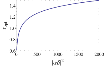
Only the noise can be slightly influenced: a numerical study of the variance of the photon distribution given in Eqs. (II) shows that $\theta=2\phi$ and $\lambda=0$ is the optimal choice. Then, one finds $\langle\Delta n_{1}^{2}\rangle=\delta^{2}|\alpha|^{2}\textnormal{e}^{-2r}+2\sinh^{2}r\cosh^{2}r$. The minimum of the variance depends on the parameter $\alpha\delta$, and in Fig. 7 we show the optimal squeezing parameter as a function of $|\delta\alpha|^{2}$. This squeezing parameter should be chosen in order to minimize photon counting uncertainties. For large squeezing parameters the distributions show characteristic oscillations Scully and Zubairy (1997).

Refer to captionRefer to captionRefer to caption
Figure 6: (Color online) Photon number probability distribution for $|\alpha\delta|^{2}=500$, $\theta=2\phi$, and different values of the squeezing parameter $r=0,~{}0.3,~{}0.6,~{}0.9,~{}1.2,~{}1.5$ in the dark port. On the right hand side of the plot we show the mean and the variance squared of these distributions.
Refer to caption
Figure 7: (Color online) Optimal squeezing parameter as a function of $|\alpha\delta|^{2}$ determined from the minimum of the variance of the distribution function.

IV Summary and conclusions

In a recent paper by Barak and Ben-Aryeh Barak and Ben-Aryeh (2008) it was suggested that due to entanglement effects in the output state of a beam splitter, the gravitational wave signal observed with an interferometer may be amplified without simultaneously increasing quantum mechanical photon counting noise.

In this paper we reanalyze such entanglement effects, and cannot confirm the significant signal amplification predicted in Ref. Barak and Ben-Aryeh (2008) but agree that consideration of such entanglement effects is important in order to calculate the photon counting noise in optical interferometers. We observe that for a strong coherent input in port 1 of the beam splitter and a squeezed vacuum injected in port 2 photon counting statistics slightly improves if the beam splitter is oriented slight off the right angle with the incoming strong coherent field. The differences between the calculations presented here and those of Ref. Barak and Ben-Aryeh (2008) can be traced to algebraic issues, which are discussed explicitly in section III.

It appears that entanglement effects must be carefully studied for any particular interferometer design, a task for which the formulas developed in the present paper may be helpful, in particular the general result Eq. (12) for the calculation of photon distributions in the output state.

Appendix A Disentangling

In order to solve the disentangling problem ($r=|\zeta|$)

$$\exp(r\hat{A})=\exp(\sigma_{T}\hat{t}_{12})\exp(\sigma_{S}\hat{s}_{12})\exp(\sigma_{1}\hat{s}_{1})\exp(\sigma_{2}\hat{s}_{2})$$ (19)

with $\hat{A}$ given in Eq. (5), we consider the Lie algebra of the operators $\left\{\hat{s}_{1},\hat{s}_{2},\hat{s}_{12},\hat{t}_{12}\right\}$ defined in Eqs. (6) and (7) with their commutators given in Eq. (II). The corresponding matrix representations of these operators

$$\hat{s}_{1}=\left(\begin{array}[]{ll}1&0\hbox{}\\ 0&0\hbox{}\end{array}\right),\quad\hat{s}_{2}=\left(\begin{array}[]{ll}0&0\hbox{}\\ 0&1\hbox{}\end{array}\right),\quad\hat{s}_{12}=\left(\begin{array}[]{ll}0&-1\hbox{}\\ -1&0\hbox{}\end{array}\right),\quad\hat{t}_{12}=\left(\begin{array}[]{ll}0&-1\hbox{}\\ 1&0\hbox{}\end{array}\right)$$ (20)

fulfill the same commutation relations.

The matrix representation of the operator $\hat{A}$ in Eq. (19) is then obtained as

$$A=\left(\begin{array}[]{ll}\sin^{2}\gamma&-\cos\gamma\sin\gamma\hbox{}\\ -\cos\gamma\sin\gamma&\cos^{2}\gamma\hbox{}\end{array}\right).$$ (21)

Since $\hat{A}^{n}=\hat{A}$ for all $n\in N$ we find for the left hand side of Eq. (19)

$$\exp(r\hat{A})=\sum_{n=0}^{\infty}{\frac{(r\hat{A})^{n}}{n!}}=\hat{I}+(\textnormal{e}^{r}-1)\hat{A}.$$ (22)

The matrix representation of the right hand side Eq. (19) is also easily calculated

$\displaystyle\exp(\sigma_{T}T_{12})\exp(\sigma_{S}\hat{s}_{12})\exp(\sigma_{1}\hat{s}_{1})\exp(\sigma_{2}\hat{s}_{2})=$ (23)
$\displaystyle\left(\begin{array}[]{ll}\textnormal{e}^{\sigma_{1}}(\sin\sigma_{T}\sinh\sigma_{S}+\cos\sigma_{T}\cosh\sigma_{S})&-\textnormal{e}^{\sigma_{2}}(\sin\sigma_{T}\cosh\sigma_{S}+\cos\sigma_{T}\sinh\sigma_{S})\hbox{}\\ \textnormal{e}^{\sigma_{1}}(\sin\sigma_{T}\cosh\sigma_{S}-\cos\sigma_{T}\sinh\sigma_{S})&-\textnormal{e}^{\sigma_{2}}(\sin\sigma_{T}\sinh\sigma_{S}-\cos\sigma_{T}\cosh\sigma_{S})\hbox{}\end{array}\right).$ (26)

By equating Eqs. (22) and (23) one obtains four equations for the four parameters ${\sigma_{T},\sigma_{S},\sigma_{1},\sigma_{2}}$ to be determined

$\displaystyle\textnormal{e}^{r}\sin^{2}\gamma+\cos^{2}\gamma$ $\displaystyle=$ $\displaystyle\textnormal{e}^{\sigma_{1}}(\sin\sigma_{T}\sinh\sigma_{S}+\cos\sigma_{T}\cosh\sigma_{S}),$
$\displaystyle(1-\textnormal{e}^{r})\cos\gamma\sin\gamma$ $\displaystyle=$ $\displaystyle-\textnormal{e}^{\sigma_{2}}(\sin\sigma_{T}\cosh\sigma_{S}+\cos\sigma_{T}\sinh\sigma_{S}),$ (27)
$\displaystyle(1-\textnormal{e}^{r})\cos\gamma\sin\gamma$ $\displaystyle=$ $\displaystyle\textnormal{e}^{\sigma_{1}}(\sin\sigma_{T}\cosh\sigma_{S}-\cos\sigma_{T}\sinh\sigma_{S}),$
$\displaystyle\textnormal{e}^{r}\cos^{2}\gamma+\sin^{2}\gamma$ $\displaystyle=$ $\displaystyle-\textnormal{e}^{\sigma_{2}}(\sin\sigma_{T}\sinh\sigma_{S}-\cos\sigma_{T}\cosh\sigma_{S}).$

This set of equations is easily solved numerically. Results are shown in Fig. 1.

For $\gamma=\pi/2$ solutions of Eqs. (A) can easily be found analytically,

$$\gamma=\pi/2,\quad\sigma_{1}=r,\quad\sigma_{2}=0,\quad\sigma_{S}=0,\quad\sigma_{T}=0.$$ (28)

If one expands the trigonometric functions on the right hand side of Eqs. (A) keeping only linear terms in the disentangling coefficients, one finds

$$\gamma=\pi/2+\delta,\quad\sigma_{1}=r,\quad\sigma_{2}=0,\quad\sigma_{S}=-\delta\sinh r,\quad\sigma_{T}=\delta(1-\cosh r).$$ (29)

For $\gamma=\pi/4$ one finds

$$\gamma=\pi/4,\quad\sigma_{1}=r/2,\quad\sigma_{2}=r/2,\quad\sigma_{S}=r/2,\quad\sigma_{T}=0.$$ (30)

Appendix B Evaluation of the entanglement factors

The entanglement factors $\exp(\sigma_{T}\hat{t}_{12})$ and $\exp(\sigma_{S}\hat{s}_{12})$ must be further transformed for convenient calculations. Using the fact that the operators $\hat{b}_{1}^{\dagger}\hat{b}_{2}^{\dagger}$, $\hat{b}_{1}\hat{b}_{2}$, and $\frac{1}{2}(1+\hat{b}_{1}^{\dagger}\hat{b}_{1}+\hat{b}_{2}^{\dagger}\hat{b}_{2})$ form an SU(1,1) Lie algebra one easily finds that

$$\exp[\sigma_{S}\hat{s}_{12}]=\exp\left(\hat{b}_{1}^{\dagger}\hat{b}_{2}^{\dagger}\textnormal{e}^{i\theta}\tanh\sigma_{S}\right)\exp\left(-\left(1+\hat{n}_{1}+\hat{n}_{2}\right)\ln(\cosh\sigma_{S})\right)\exp\left(-\hat{b}_{1}\hat{b}_{2}\textnormal{e}^{-i\theta}\tanh\sigma_{S}\right).$$ (31)

as was proved e.g. in Ref. DasGupta (1996). Similarly one proves that

$$\exp[\sigma_{T}\hat{t}_{12}]=\exp\left(\hat{b}_{1}\hat{b}_{2}^{\dagger}\textnormal{e}^{i\theta}\tan\sigma_{T}\right)\exp\left(-\left(\hat{n}_{1}-\hat{n}_{2}\right)\ln(\cos\sigma_{T})\right)\exp\left(-\hat{b}_{1}^{\dagger}\hat{b}_{2}\textnormal{e}^{-i\theta}\tan\sigma_{T}\right).$$ (32)

using the fact that the operators $\hat{b}_{1}\hat{b}_{2}^{\dagger}$, $\hat{b}_{1}^{\dagger}\hat{b}_{2}$, and $-\frac{1}{2}\left(\hat{b}_{1}^{\dagger}\hat{b}_{1}-\hat{b}_{2}^{\dagger}\hat{b}_{2}\right)$ form an SU(2) Lie algebra. Expanding out the exponentials in the expressions above allows for convenient application of these operators on Fock states.

Appendix C Transformations

The following transformations for products of displacement operators and squeezing operators can be easily proved from the Baker-Campbell-Haussdorff theorem and the Boson commutation relations,

$\displaystyle\hat{D}(\alpha_{2})\hat{D}(\alpha_{1})$ $\displaystyle=$ $\displaystyle\hat{D}(\alpha_{1}+\alpha_{2})\exp\left[\frac{1}{2}(\alpha_{2}\alpha_{1}^{*}-\alpha_{2}^{*}\alpha_{1})\right],$
$\displaystyle\hat{D}(\alpha)\hat{S}(\zeta)$ $\displaystyle=$ $\displaystyle\hat{S}(\zeta)\hat{D}(\alpha\cosh r+\alpha^{*}\textnormal{e}^{i\theta}\sinh r),\quad\zeta=r\textnormal{e}^{i\theta}.$ (33)

These relations are used to obtain Eq. (15).


Acknowledgements

We would like to thank Yacob Ben-Aryeh for a useful correspondence and a critical reading of the manuscript. M. W. acknowledges Roman Schnabel for a useful correspondence and Robert Wynands for useful discussions on experimental issues. V.G.V. thanks Physikalisch-Technische Bundesanstalt for support of an internship, while this work was performed.

References

  • Caves (1981) C. M. Caves, Phys. Rev. D 23, 1693 (1981).
  • Yurke et al. (1987) B. Yurke, P. Grangier, and R. Slusher, J. Opt. Soc. Am. B 4, 1677 (1987).
  • Assaf and Ben-Aryeh (2002) O. Assaf and Y. Ben-Aryeh, J. Opt. Soc. Am. B 19, 2716 (2002).
  • Barak and Ben-Aryeh (2008) R. Barak and Y. Ben-Aryeh, J. Opt. Soc. Am. B 25, 361 (2008).
  • Campos et al. (1989) R. A. Campos, B. E. A. Saleh, and M. C. Teich, Phys. Rev. A 40, 1371 (1989).
  • Wei and Norman (1963) J. Wei and E. Norman, J. Math. Phys. 4, 575 (1963).
  • Scholz et al. (2010) D. Scholz, V. G. Voronov, and M. Weyrauch, to be published (2010).
  • Scully and Zubairy (1997) M. O. Scully and M. S. Zubairy, Quantum Optics (Cambridge University Press, Cambride, U.K., 1997), 1st ed.
  • Mehmet et al. (2009) M. Mehmet, H. Vahlbruch, N. Lastzka, K. Danzmann, and R. Schnabel, arXiv:0909.5386 (2009).
  • DasGupta (1996) A. DasGupta, Am. J. Phys. 64, 1422 (1996).