Chaos of the logistic equation with piecewise constant argument

Abstract

We consider the logistic equation with different types of the piecewise constant argument. It is proved that the equation generates chaos and intermittency. Li-Yorke chaos is obtained as well as the chaos through period-doubling route. Basic plots are presented to show the complexity of the behavior.

1 Introduction

The first papers about simple population models with complex dynamics are [1, 2]. The main method of analysis of these models is the reduction to discrete equations: the logistic and Ricker’s equation [4].

In [3], Liu and Gopalsamy investigated the following equation with piecewise constant argument

$$\frac{d\,x(t)}{dt}=r\,x(t)\,\Big{\{}1-a\,x(t)-b\,x([t])\Big{\}},\>\>\>t>0,$$ (1)

where $r,a,b$ are positive constants and $[.]$ denotes the greatest integer function. The authors showed that for certain parameter values of $a$ and $b$, equation (1) generates Li-Yorke chaos [5].

In the present paper the approaches of [1, 2] and [3] are developed for different types of the logistic equation with piecewise constant argument. Transformations of the dependent and independent variables are used to obtain convenient discrete equations for the dynamic analysis. The Li-Yorke theorem [5] is referred to prove chaos. A connection between solutions of continuous models and discrete equations is used to make appropriate simulations.

In the paper following equations are considered:

$$\frac{d\,x(t)}{dt} = (a-b\,x([t]))\,x([t]),$$ (2)

$$\frac{d\,x(t)}{dt} = (a-b\,x([t+1]))\,x(t),$$ (3)

$$\frac{d\,x(t)}{dt} = (a-b\,x([t+1]))\,x([t+1]).$$ (4)

It is seen that we suggest to involve not only delayed, but also advanced arguments in the population models. Although the role of delay in the population dynamics has been discussed vitally [6], the anticipation phenomena has not been considered yet. Anticipatory assumption in a population model may mean that a will, a wish, an anticipation is taken into account. It can be assumed that anticipation is a prediction reached by the decisions of the present time. We introduce anticipation in our population models via function $[t+1]$ [7].

We show that for critical values of the parameters $a,b$ the solutions of the differential equations (2),(3),(4) show intermittency which is “almost periodic” behavior interrupted by chaotic motions [8, 9].

In the population models, we consider $x(t)=N(t)-N_{0}$, where $N(t)$ denotes the size of the population at time $t$ and $N_{0}$ is a positive integer, let say, the average value of a population. Thus, $x$ does not represent the size of the population and it can be negative.

2 Analysis of the equations

Let us start with equation (2). If $t\in[k,k+1)$, $k\in\mathbb{N}_{0}$, it takes the following form

$$\frac{d\,x(t)}{dt}=(a-b\,x_{k})\,x_{k},$$ (5)

then,

$$x(t)=x_{k}+(a-b\,x_{k})\,x_{k}\,(t-k),$$ (6)

and, hence

$$x_{k+1}=x_{k}\,(1+a-b\,x_{k}).$$ (7)

If one makes the change of variable $q_{k}=\frac{b}{1+a}\,x_{k}$ in (7), then obtains

$$q_{k+1}=\mu\,q_{k}\,(1-q_{k}),$$ (8)

where $\mu=1+a$. The right-hand side of equation (8) is the logistic map

$$G(q)=\mu\,q\,(1-q).$$ (9)

When $\mu\cong 3.57$, $G$ generates chaos through period-doubling (see [10] for more details). Since this map is obtained from the solution of the equation (5) and $\mu=1+a$, it is obvious that equation (2) can generate chaos for $a\cong 2.57$.

In [10], one can find that $G$ has intermittent behavior at $\mu=3.8282$. Therefore, equation (6), and consequently, (2), displays intermittency, too.

Let $a=2.8282$, $b=1/50$ and $x(0)=56.7148$. One can see the intermittency phenomena for equation (2) in Figure 1.

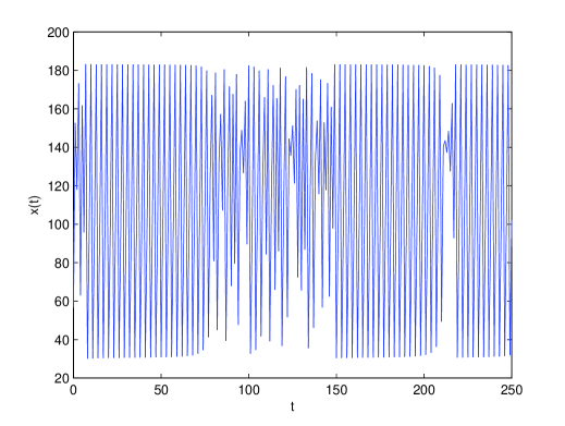
Figure 1: The solution of the differential equation $\frac{d\,x(t)}{dt}=(a-b\,x([t]))\,x([t])$ with $x(0)=56.7148$, $a=2.8282$, $b=1/50$.

Let us consider another equation (3). If $t\in[k,k+1)$, then

$$\frac{d\,x(t)}{dt}=(a-b\,x_{k+1})\,x(t),$$ (10)

and

$$x(t)=x_{k}\,e^{\int_{k}^{t}(a-b\,x_{k+1})\,ds}.$$ (11)

Hence,

$$x_{k}=x_{k+1}\,e^{(b\,x_{k+1}-a)}\>\>\>(k\in\mathbb{N}_{0}).$$ (12)

Now the transformation $k=-n$, $r_{n}=-x_{1-n}$, in (12) yields

$$r_{n+1}=r_{n}\,e^{-b\,r_{n}-a},$$ (13)

where $n$ is a negative integer. The right-hand side of equation (13) is a function of the form

$$T(r)=r\,e^{-a-b\,r}.$$

In their article, May and Oster [1] discussed the behavior of the following discrete-time equation:

$$X_{t+1}=X_{t}\,e^{\gamma\,(1-X_{t})},\>\>\>\gamma>0.$$ (14)

They proved that for certain values of $\gamma$ equation (14) has fixed points of period $k$ for $k=1,2,3,\ldots$ and it generates chaos. Below we will try to extend their results to equation (11) for $a=-\gamma$ and $b=0.01$.

Now let us consider the fixed points of $T$, $T^{2}$ and $T^{3}$ for different values of $a$ with $b=0.01$. Consider the value $a_{c}=-3.102$ which is borrowed from [1], the mapping $T^{3}$ is tangent to $y=r$ line, as shown in Figure 2.

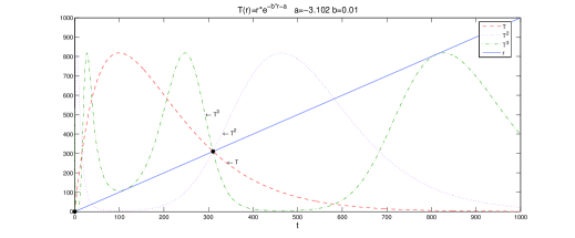
Figure 2: The graphs of $T(r),\,T^{2}(r),\,T^{3}(r)$ and $y=r$ when $a=-3.102$ and $b=0.01$.

When $a=-3.15$, the mapping $T^{3}$ has extra fixed points which are denoted by black stars in Figure 3. Then, there exist period three points which are not period one and two. Consequently, equation (3) admits the chaos through Li and Yorke theorem [5].

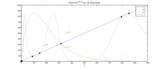
Figure 3: The graphs of $T(r),\,T^{2}(r),\,T^{3}(r)$ and $y=r$ when $a=-3.15$ and $b=0.01$.

For values of $a$ just above $a_{c}$, the system displays intermittency. In common, simulations of the corresponding discrete equation (13) are realized, but we propose to see the complex behavior in its original form. Thus, to compute $x(t)$ for $t\geq 0$ let us apply the following program. First, we fix $r_{n}$ with a negative integer $n$. Then, we calculate the sequence $\left\{r_{n+1},r_{n+2},\ldots,r_{1},r_{0}\right\}$, by using (13) and, then $k=-n$, $r_{n}=-x_{1-n}$ and $x_{0}=x_{1}\,e^{(b\,x_{1}-a)}$. Substituting values of $x_{k}$ and $x_{k+1}$ in (11), we obtain the solution of equation (10). When $a=-3.1$, $b=0.01$ and $r_{-150}=5$, the result of simulation is seen in the Figure 4.

Figure 4: The graph of $x(t)$ for $a=-3.1$, $b=0.01$, $x_{151}=-5$.

Let $a_{\infty}=-2.6924...$ and $b=0.01,\>r_{-50}=70.2344$. In Figure 5, one can see that equation (11) generates chaos.

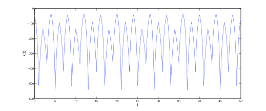
Figure 5: The graph of $x(t)$ for $a_{\infty}=-2.6924...$ and $b=0.01,\>x_{51}=-70.2344$.

Our last system is as follows

$$\frac{d\,x(t)}{dt}=(a-b\,x([t+1]))\,x([t+1]),$$ (15)

where $a$ and $b$ are constants with $a\neq 1.$ The corresponding discrete-time equation is

$$x_{k}=x_{k+1}(1-a+b\,x_{k+1}),\>\>\>(k\in\mathbb{N}_{0}).$$ (16)

Let $k=-n$ and $r_{n}=\frac{b}{a-1}\,x_{1-n}$, the last equation can be written in the following form

$$r_{n+1}=(1-a)\,r_{n}\,(1-r_{n}),$$ (17)

where $n$ is a negative integer. The right-hand side of equation (17) is a function of the form $P(r)=\mu\,r\,(1-r),$ where $\mu=1-a$. Similarly to the equation (9), the last one generates complex dynamics.

3 Conclusion

We discuss the complex behavior of different types of logistic equations with piecewise constant argument of delay and advance types. The idea of anticipation and piecewise constant argument are used together. Transformations of the space and time variables are used to obtain proper discrete-time equations. The parameter values of the discrete-time equations which cause chaos and intemittency are utilized to get analogues for continuous solutions. Simulations of the continuous dynamics are given.

References

- [1] R. May, G. F. Oster, Bifurcations and dynamic complexity in simple ecological models, Am. Nat. 110 (1976) 573-599.
- [2] R. May, Simple mathematical models with very complicated dynamics, Nature 261 (1976) 459-467.
- [3] P. Liu, K. Gopalsamy, Global stability and chaos in a population model with piecewise constant arguments, Appl. Math. Comput. 101 (1999) 63-88.
- [4] W. E. Ricker, Stock and recruitment, J. Fish. Res. Board Can. 11 (1954) 559-623.
- [5] T.-Y. Li, J. A. Yorke, Period three implies chaos, Amer. Math. Monthly 82 (1975) 985-992.
- [6] J. D. Murray, Mathematical biology, New York: Springer, 2003.
- [7] M. U. Akhmet, H. Öktem, S. Pickl, G. W. Weber, An anticipatory extension of Malthusian model, Seventh International Conference on Computing Anticipatory Systems, Computing Anticipatory System, CASYS05, 2006, pp. 260-264.
- [8] Y. Pomeau, P. Manneville, Intermittent transition to turbulence in dissipative dynamical systems, Commun. Math. Phys. 74 (1980) 189-197.
- [9] J. E. Hirsch, B. A. Huberman, D. J. Scalapino, Theory of intermittency, Phys. Rev. A 25 (1982) 519-532.
- [10] S. H. Strogatz, Nonlinear dynamics and Chaos: with applications to physics, biology, chemistry, and engineering, Reading, Mass.: Addison- Wesley Pub., 1994.