Anisotropic Poisson Processes of Cylinders

Abstract

Main characteristics of stationary anisotropic Poisson processes of cylinders (dilated $k$-dimensional flats) in $d$-dimensional Euclidean space are studied. Explicit formulae for the capacity functional, the covariance function, the contact distribution function, the volume fraction, and the intensity of the surface area measure are given which can be used directly in applications.

Keywords porous media, fiber process, anisotropy, intrinsic volumes, stochastic geometry
Mathematics Subject Classification (2000) 60D05 60G10

1 Introduction

Porous fiber materials find vast applications in modern material technologies. Their use ranges from light polymer-based non-woven materials, see Helfen et al (2003), to fiber-reinforced textile and fuel cells as in Mukherjee and Wang (2006). Their porosity, percolation, acoustic absorption and liquid permeability are of special interest. It is known that these properties depend to a great extent on the microscopic structure of fibers, in particular, on the orientation of a typical fiber. If all directions of fibers are equiprobable one speaks of isotropy. Many materials are made by pressing an isotropic collection of fibers together thus producing strongly anisotropic structures. As examples, pressed non-woven materials used as an acoustic trim in car production, see Schladitz et al (2006), paper making process as in Corte and Kallmes (1962), and Molchanov et al (1993), and gas diffusion layers of fuel cells, here Mathias et al (2003), Manke et al (2007) can be mentioned; see Figure 1.

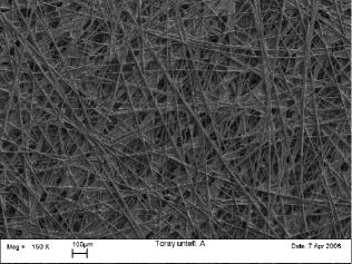
Figure 1: Microscopic structure of the gas diffusion layer as used in polymer electrolyte membrane fuel cells (courtesy of the Centre for Solar Energy and Hydrogen Research, Ulm)

To quantify this dependence between the physical and the geometric structural properties of porous materials, their intrinsic volumes (sometimes also called Minkowski functionals or quermassintegrals) are used. More formally, porous fiber materials are usually modeled as homogeneous random closed sets described in Matheron (1975) and Serra (1982). The mean volume and surface area of such sets in an observation window averaged by the volume of the window are examples of intensities of intrinsic volumes which are treated in detail in this paper.

The intention of this paper is to give formulae for cylinder processes which can be used directly in applications, which is also demonstrated in the optimization example. Thus the focus is on stationary Poisson processes which are the most common in applications. A rather theoretical analysis can be found in the recent paper by Hoffmann (2009), where formulae for the curvature measures of a more general non-stationary model of Poisson cylinder processes can be found. In Weil (1987) the model for cylinders as used in this paper is introduced, and curvature measures for different kinds of (not necessarily Poisson) point processes are calculated. As opposed to that, in this paper formulae for the covariance function, the contact distribution function, and a different approach for the calculation of the specific surface area of Poisson cylinder processes are worked out which have straightforward applied value.

As a model for fiber materials shown in Figure 1, we consider anisotropic stationary cylinder processes as homogeneous Poisson point processes in the space of cylinders. Isotropic models of this kind (named also processes of “thick” fibers, lamellae, membranes or Poisson slices) have been studied in detail, cf. Matheron (1975), Serra (1982), Davy (1978), Ohser and Mücklich (2000). See Schneider (1987) for further references. In the present paper, we generalize some of their results to the anisotropic case.

After giving some preliminaries on cylinder processes (Section 2), we obtain formulae for the capacity functional, covariance function and contact distribution function in Section 3. In Section 4, we prove the formulae for the intensity of the surface area measure of anisotropic stationary Poisson processes of cylinders. Formulae for the intensities of other intrinsic volumes can be found in the recent paper by Hoffmann (2009). In the last section, we show how the volume fraction of an anisotropic Poisson process of cylinders can be maximized under certain constraints. In the solution, we use the formulae obtained in previous sections.

Since the formulae obtained in Sections 3–4 are rather complex, examples in the most interesting dimensions 2 and 3 are given, which can be directly used in applications.

2 Cylinder Processes

Let $G(k,d)$ be the Grassmann manifold of all non-oriented $k$-dimensional linear subspaces of $\mathbb{R}^{d}$, and $\mathfrak{G}$ the $\sigma$-algebra of Borel subsets of $G(k,d)$ in its usual topology. Let $\mathcal{C}$ $(\mathcal{K})$ be the set of all compact (compact convex) non-empty sets in $\mathbb{R}^{d}$. Denote by $\mathcal{R}$ the convex ring, i.e., the family of all finite unions of non-empty compact convex sets. We provide these sets with the Hausdorff metric, and denote the resulting Borel $\sigma$-algebra of $\mathcal{R}$ by $\mathfrak{R}$.

Denote by $\nu_{k}(\cdot)$ the $k$-dimensional Lebesgue measure in $\mathbb{R}^{k}$, and by $\mathcal{H}^{k}(\cdot)$ the $k$-dimensional Hausdorff measure. For any set $S\subset\mathbb{R}^{d}$ denote by $S^{\perp}$ the linear subspace of the vectors which are orthogonal to all elements of $S$. For $\xi$ being a $k$-dimensional flat (i.e. a $k$-dimensional linear subspace) we denote the $(d-k)$-dimensional Lebesgue measure in $\xi^{\perp}$ by $\nu_{d-k}^{\xi}$. Let $\kappa_{k}$ ($\omega_{k}$) be the volume (surface area) of a unit $k$-dimensional ball, respectively.

For a convex set $K\in\mathcal{K}$ and $\mathbf{x}\in\mathbb{R}^{d}$ let $p(K,\mathbf{x})$ be the unique point in $K$ which is the closest to $\mathbf{x}$. Then there exist measures $\Phi_{k}(K,\cdot)$ on $\mathcal{B}(\mathbb{R}^{d})$, for $k=0,\dots,d$ with

$$\nu_{d}(\{\mathbf{x}\in K\oplus B_{r}(\mathbf{o}):p(K,\mathbf{x})\in B\})=\sum_{k=0}^{d}r^{d-k}\kappa_{d-k}\Phi_{k}(K,B),$$

where $K_{1}\oplus K_{2}=\{k_{1}+k_{2}|k_{1}\in K_{1},k_{2}\in K_{2}\}$, and $B_{r}(o)$ is the ball of radius $r$ centered in the origin $o$. Furthermore we define $\Phi_{k}(\emptyset,B)=0$ for all $B\in\mathcal{B}(\mathbb{R}^{d})$. These measures are called curvature measures. Since they are locally determined, they can be extended to functions with locally polyconvex sets as first argument in such a way that they remain additive. One should remark that these generalized curvatures measures are not necessarily positive, but signed measures. For a detailed introduction, see Schneider and Weil (2008). The intrinsic volumes of $K$ can be defined as total curvature measures $V_{k}^{d}(K)=\Phi_{k}(K,\mathbb{R}^{d})$ for $k=0,\ldots,d$.

Following the approach introduced in Weil (1987), we define a cylinder as the Minkowski sum of a flat $\xi\in G(k,d)$ and a set $K\subset\xi^{\perp}$ with $K\in\mathcal{R}$. Note that $K$ is not limited to sets with an associated point in the origin. The flat $\xi$ is also called the direction space of $\xi\oplus K$ and $K$ is called the cross section or base. For a cylinder $Z=K\oplus\xi$ we define the functions $L(Z)=\xi$ and $K(Z)=K$. Furthermore, define $\mathcal{Z}_{k}$ as the set of all cylinders which have a $k$-dimensional direction space and base in $\mathcal{R}$. For the volume of the cross-section of the cylinder we introduce the notation $A(Z)=\nu_{d-k}^{L(Z)}(K(Z))$. By $S(K)$ we denote the surface area of a set $K$. In the case of $K$ being the cross-section of a cylinder $K\oplus L$ we shall use this notation for the surface area of $K$ in the space $L^{\perp}$.

We call a measure $\varphi$ on $\mathcal{Z}_{k}$ locally finite if $\varphi(\{Z\in\mathcal{Z}_{k}|Z\cap K\neq\emptyset\})<\infty$ for all $K\in\mathcal{C}$. Let $\mathcal{M}(\mathcal{Z}_{k})$ be the set of locally finite counting measures on $\mathcal{Z}_{k}$ supplied with the usual $\sigma$-algebra $\mathfrak{M}$. A point process $\Xi$ on $\mathcal{Z}_{k}$ which is a measurable mapping from a probability space $(\Omega,\mathcal{F},\textbf{P})$ into $(\mathcal{M}(\mathcal{Z}_{k}),\mathfrak{M})$ is called a cylinder process. Its distribution is given by the probability measure $\textbf{P}_{\Xi}\colon\mathfrak{M}\to[0,1]$, $\textbf{P}_{\Xi}(\cdot)=\textbf{P}(\Xi\in\cdot)$. A cylinder process is called Poisson if $\Xi(B)$ is Poisson distributed with mean $\Lambda(B)$ for some locally finite measure $\Lambda$ on $\mathcal{Z}_{k}$ and all Borel sets $B\subset\mathcal{Z}_{k}$, and $\Xi(B_{1}),\Xi(B_{2}),\dots,\Xi(B_{n})$ are independent for all disjoint Borel sets $B_{1},B_{2},\dots,B_{n}\subset\mathcal{Z}_{k}$, and all $n\geq 2$, see details in Schneider and Weil (2008). The measure $\Lambda$ is called the intensity measure of $\Xi$. The Poisson cylinder process is called simple, if it has no multiple points. This is the case if and only if $\Lambda$ is diffuse. For the rest of this paper we assume that $\Xi$ is a simple Poisson cylinder process. In this case, the union $U_{\Xi}=\cup_{Z\in\Xi}Z$ is a random closed set, see (Schneider and Weil, 2008, p. 96), where we denote by $Z\in\Xi$ the cylinders $Z$ in the support set of $\Xi$.

The cylinder process $\Xi$ is called stationary if its distribution is invariant with respect to translations in $\mathbb{R}^{d}$ and isotropic if it is invariant w.r.t. rotations about the origin. Let $\mathcal{Z}_{k}^{o}$ be the set of all cylinders $K\oplus\xi$ with $\xi\in G(k,d),K\subset\xi^{\perp}$, and for which the midpoint of the circumsphere of $K$ lies in the origin.

Following Weil (1987), we define $i\colon(\mathbf{x},Z)\mapsto\mathbf{x}+Z$ for $\mathbf{x}\in\mathbb{R}^{d}$ and $Z\in\mathcal{Z}_{k}^{o}$. If $\Xi$ is stationary, then a number $\lambda\geq 0$ and a probability measure $\theta$ on $\mathcal{Z}_{k}^{o}$ exist such that

$$\Lambda(i(A\times C))=\lambda\int_{C}\nu_{d-k}^{L(Z)}(A)\theta(\textup{d}Z)$$

for all Borel sets $A\subset\mathbb{R}^{d},C\subset\mathcal{Z}_{k}^{o}$. Then $\lambda$ is called the intensity and $\theta$ the shape distribution of $\Xi$.

As shown in (König and Schmidt, 1991, p. 61), $\theta$ can be decomposed further. Analogously to $i$ define $j\colon(\varrho\times\xi)\mapsto\varrho\oplus\xi$ for $\varrho\in\mathcal{R}$ and $\xi\in G(k,d)$. Then there exist a probability measure $\alpha$ on $\mathfrak{G}$ (directional distribution of $\Xi$) and a probability kernel $\beta\colon\mathfrak{R}\times G(k,d)\to[0,1]$ for which $\beta(\cdot,\xi)$ is concentrated on subsets of $\xi^{\perp}$ such that for arbitrary $R\in\mathfrak{R}$ and $G\in\mathfrak{G}$ the equation

$$\theta(j(R\times G))=\int_{G}\beta(R,\xi)\alpha(\textup{d}\xi)$$ (1)

holds.

3 Capacity functional and related characteristics

In this section, we calculate the capacity functional (cf. (Stoyan et al, 1995, p. 195)) for the union set $U_{\Xi}$ of the stationary Poisson process $\Xi$ of cylinders with $k$-dimensional direction space introduced as above. As a corollary, explicit formulae for the volume fraction, the covariance function, and the contact distribution function of $U_{\Xi}$ follow easily. It is worth mentioning that the resulting formula (2) for the capacity functional generalizes the formula in (Serra, 1982, pp. 572-573), given for Poisson slices in $\mathbb{R}^{3}$, and a model with this capacity functional has already been proposed in (Matheron, 1975, p. 148).

3.1 Capacity functional

For any random closed set $X$, the capacity functional $T_{X}(B)=\textbf{P}(X\cap B\neq\emptyset),B\in\mathcal{C}$, determines uniquely the distribution of $X$.

Let $\pi_{\eta}(B)$ be the orthogonal projection of a set $B\subset\mathbb{R}^{d}$ along a linear subspace $\eta\subset\mathbb{R}^{d}$ onto $\eta^{\perp}$.

Lemma 1.

The capacity functional of the union set $U_{\Xi}$ of the cylinder process $\Xi$ is given by

$$T_{U_{\Xi}}(B)=1-\exp\left\{-\lambda\int_{\mathcal{Z}_{k}^{o}}\nu_{d-k}^{L(Z)}(-K(Z)\oplus{\pi}_{L(Z)}(B))\,\theta(\textup{d}Z)\right\}.$$ (2)

Proof.

Let $B$ be a compact set in $\mathbb{R}^{d}$. Then by Fubini’s theorem and (Schneider and Weil, 2008, p. 96), we get

$$1-T_{U_{\Xi}}(B) =\exp\{-\Lambda(\{Z\in\mathcal{Z}_{k}|Z\cap B\neq\emptyset\})\}=\exp\left\{-\int_{\mathcal{Z}_{k}}\mathbf{1}\{\tilde{Z}\cap B\neq\emptyset\}\Lambda(\textup{d}\tilde{Z})\right\}$$

$$=\exp\left\{-\lambda\int_{\mathcal{Z}_{k}^{o}}\int_{L(Z)^{\perp}}\mathbf{1}\{(Z+\mathbf{x})\cap B\neq\emptyset\}\,\textup{d}\mathbf{x}\,\theta(\textup{d}Z)\right\}$$

$$=\exp\left\{-\lambda\int_{\mathcal{Z}_{k}^{o}}\int_{L(Z)^{\perp}}\mathbf{1}\{(K(Z)+\mathbf{x})\cap{\pi}_{L(Z)}(B)\neq\emptyset\}\,\textup{d}\mathbf{x}\,\theta(\textup{d}Z)\right\},$$

where $\tilde{Z}=\mathbf{x}+Z$.

One can easily see that $K(Z)+\mathbf{x}$ hits ${\pi}_{L(Z)}(B)$ if and only if $\mathbf{x}$ belongs to the Minkowski sum of $-K(Z)$ and ${\pi}_{L(Z)}(B)$.

Thus we have

$$1-T_{U_{\Xi}}(B) =\exp\left\{-\lambda\int_{\mathcal{Z}_{k}^{o}}\int_{L(Z)^{\perp}}\mathbf{1}\{(K(Z)+\mathbf{x})\cap{\pi}_{L(Z)}(B)\neq\emptyset\}\,\textup{d}\mathbf{x}\,\theta(\textup{d}Z)\right\}$$

$$=\exp\left\{-\lambda\int_{\mathcal{Z}_{k}^{o}}\int_{L(Z)^{\perp}}\mathbf{1}\{\mathbf{x}\in-K(Z)\oplus{\pi}_{L(Z)}(B)\}\,\textup{d}\mathbf{x}\,\theta(\textup{d}Z)\right\}$$

$$=\exp\left\{-\lambda\int_{\mathcal{Z}_{k}^{o}}\nu_{d-k}^{L(Z)}(-K(Z)\oplus{\pi}_{L(Z)}(B))\,\theta(\textup{d}Z)\right\}.$$

∎

A few remarks are in order.

• It follows from the local finiteness of $\Lambda$ that

  $$\int_{\mathcal{Z}_{k}^{o}}\nu_{d-k}^{L(Z)}(-K(Z)\oplus{\pi}_{L(Z)}(B))\,\theta(\textup{d}Z)<\infty,$$ (3)

  cf. (Schneider and Weil, 2008, p. 96, Theorem 3.6.3. and remark).

• The choice of $k=0$ yields the capacity functional of the stationary Boolean Model $\Xi^{\prime}$ with the primary grain $K$ and intensity $\lambda$, cf. (Matheron, 1975, p. 62):

  $$T_{\Xi^{\prime}}(B)=1-\textup{e}^{-\lambda E\nu_{d}(-K\oplus B)}\,.$$

• Another important special case is that of $K$ being a.s. a point. Then the model coincides with a $k$-flat process $\Xi^{\prime\prime}$, cf. (Matheron, 1975, p. 67) with the capacity functional

  $$T_{\Xi^{\prime\prime}}(B)=1-\exp\left\{-\lambda\int_{\mathcal{Z}_{k}^{o}}\nu_{d-k}^{L(Z)}({\pi}_{L(Z)}(B))\,\theta(\textup{d}Z)\right\}.$$

• The case of $B=\{\mathbf{o}\}$ yields the volume fraction $p=\textbf{P}(\mathbf{o}\in U_{\Xi})=\linebreak E\nu_{d}(U_{\Xi}\cap[0,1]^{d})$ of $U_{\Xi}$:

  $$p=T_{U_{\Xi}}(\{\mathbf{o}\})=1-\exp\left\{-\lambda\int_{\mathcal{Z}_{k}^{o}}A(Z)\,\theta(\textup{d}Z)\right\}.$$ (4)

  A generalization of this formula can also be found in Hoffmann (2009) in the non-stationary setting.

  Throughout this paper, we assume that $p>0$, i.e. $\int_{\mathcal{Z}_{k}^{o}}A(Z)\theta(\textup{d}Z)>0$. Thus, we have $p\in(0,1)$, cf. inequality (3).

3.2 Covariance function

In the following we investigate the covariance function of $U_{\Xi}$. It is defined as$C_{U_{\Xi}}(\mathbf{h})=\textbf{P}(\mathbf{o},\mathbf{h}\in\Xi)$, $\mathbf{h}\in\mathbb{R}^{d}$, cf. (Stoyan et al, 1995, p. 68).

Because of the relation $C_{U_{\Xi}}(\mathbf{h})=\textbf{P}(\mathbf{o},\mathbf{h}\in\Xi)=2p-T_{U_{\Xi}}(\{\mathbf{o},\mathbf{h}\})$ it is closely connected with the capacity functional of the set $B=\{\mathbf{o},\mathbf{h}\}$, which is

$$T_{U_{\Xi}}(\{\mathbf{o},\mathbf{h}\})=1-\exp\left\{-\lambda\int_{\mathcal{Z}_{k}^{o}}\nu_{d-k}^{L(Z)}(\{\mathbf{o},{\pi}_{L(Z)}(\mathbf{h})\}\oplus-K(Z))\,\theta(\textup{d}Z)\right\}.$$ (5)

Let $\gamma_{A}$ denote the covariogram of a measurable set $A\subset L(Z)^{\perp}$ defined by

$$\gamma_{A}(\mathbf{x})=\nu_{d-k}^{L(Z)}(A\cap(A-\mathbf{x}))$$

for $\mathbf{x}\in L(Z)^{\perp}$.

Lemma 2.

For $\mathbf{h}\in\mathbb{R}^{d}$ we have

$$\begin{split}C_{U_{\Xi}}(\mathbf{h})=&\ 1-2\exp\left\{-\lambda\int_{\mathcal{Z}_{k}^{o}}A(Z)\,\theta(\textup{d}Z)\right\}\\ &\ +\exp\left\{-2\lambda\int_{\mathcal{Z}_{k}^{o}}A(Z)\,\theta(\textup{d}Z)+\lambda\int_{\mathcal{Z}_{k}^{o}}\gamma_{K(Z)}({\pi}_{L(Z)}(\mathbf{h}))\,\theta(\textup{d}Z)\right\}.\end{split}$$ (6)

Proof.

Consider the term $\{\mathbf{o},{\pi}_{L(Z)}(\mathbf{h})\}\oplus-K(Z)=-K(Z)\cup({\pi}_{L(Z)}(\mathbf{h})-K(Z))$. Its volume is equal to

$$\ \nu_{d-k}^{L(Z)}(-K(Z)\oplus\{\mathbf{o},{\pi}_{L(Z)}(\mathbf{h})\})$$

$$= \ 2A(Z)-\nu_{d-k}^{L(Z)}(K(Z)\cap(K(Z)-{\pi}_{L(Z)}(\mathbf{h})))$$

$$= \ 2A(Z)-\gamma_{K(Z)}({\pi}_{L(Z)}(\mathbf{h})).$$

Using equations (4) and (5), the covariance $C_{U_{\Xi}}(\mathbf{h})$ rewrites

$$C_{U_{\Xi}}(\mathbf{h})= \ 2p-T_{U_{\Xi}}(\{\mathbf{o},\mathbf{h}\})$$

$$= \ 1-2\exp\left\{-\lambda\int_{\mathcal{Z}_{k}^{o}}A(Z)\,\theta(\textup{d}Z)\right\}$$

$$+\exp\left\{-\lambda\int_{\mathcal{Z}_{k}^{o}}\nu_{d-k}^{L(Z)}(-K(Z)\oplus\{\mathbf{o},{\pi}_{L(Z)}(\mathbf{h})\})\,\theta(\textup{d}Z)\right\}$$

$$= \ 1-2\exp\left\{-\lambda\int_{\mathcal{Z}_{k}^{o}}A(Z)\,\theta(\textup{d}Z)\right\}$$

$$\ +\exp\left\{-2\lambda\int_{\mathcal{Z}_{k}^{o}}A(Z)\,\theta(\textup{d}Z)+\lambda\int_{\mathcal{Z}_{k}^{o}}\gamma_{K(Z)}({\pi}_{L(Z)}(\mathbf{h}))\,\theta(\textup{d}Z)\right\}.$$

∎

Example.

In the following, we give an example of a cylinder process in two dimensions with cylinders of constant thickness $2a$ where the integrals in (6) can be calculated explicitly.

Let $l$ be an arbitrary line through the origin, $\varphi$ the angle between the $x$-axis and $l^{\perp}$, and $\mathbf{h}=(r,\psi)$ a vector in polar coordinates. We use the notation $B_{a}(\mathbf{o})\times\varphi$ with $\varphi\in[0,\pi)$ for a cylinder with radius $a$ and direction space $l$. Since $|{\pi}_{l}(\mathbf{h})|=r|\cos(\varphi-\psi)|$, formula (6) rewrites

$$C_{U_{\Xi}}(\mathbf{h})=1-2\textup{e}^{-2\lambda a}+\textup{e}^{-4\lambda a+\lambda I},$$

where

$$I =\int_{0}^{\pi}(2a-|{\pi}_{l}(\mathbf{h})|)\mathbf{1}\{|{\pi}_{l}(\mathbf{h})|\leq 2a\}\,\theta(B_{a}(\mathbf{o})\times\textup{d}\varphi)$$

$$=\int_{\varphi\in[0,\pi]:|\cos(\varphi-\psi)|\leq\frac{2a}{r}}(2a-r|\cos(\varphi-\psi)|)\,\theta(B_{a}(\mathbf{o})\times\textup{d}\varphi).$$

In the isotropic case ($\theta(B_{a}(\mathbf{o})\times\textup{d}\varphi)=\textup{d}\varphi/\pi$) we can choose $\psi$ arbitrarily, for example $\psi=\pi/2$. This yields

$$I=\int_{\varphi\in[0,\pi]:\sin\varphi\leq\frac{2a}{r}}(2a-r\sin\varphi)\frac{\textup{d}\varphi}{\pi}.$$

In case $r\leq 2a$ this simplifies to

$$I=2a-r\int_{0}^{\pi}\sin\varphi\frac{\textup{d}\varphi}{\pi}=2a-r\frac{2}{\pi}.$$

And for $r>2a$ we get

$$I= \ \frac{2a}{\pi}\left(\int_{0}^{\arcsin\frac{2a}{r}}\textup{d}\varphi+\int_{\pi-\arcsin\frac{2a}{r}}^{\pi}\textup{d}\varphi\right)+$$

$$+\frac{r}{\pi}\left(\int_{0}^{\arcsin\frac{2a}{r}}(-\sin\varphi)\,\textup{d}\varphi+\int_{\pi-\arcsin\frac{2a}{r}}^{\pi}(-\sin\varphi)\,\textup{d}\varphi\right)$$

$$= \ \frac{4a}{\pi}\arcsin\left(\frac{2a}{r}\right)+\frac{2r}{\pi}\left(\cos\left(\arcsin\left(\frac{2a}{r}\right)\right)-1\right)$$

$$= \ 2a-\frac{4a}{\pi}\arccos\left(\frac{2a}{r}\right)-\frac{2r}{\pi}\left(1-\sqrt{1-\left(\frac{2a}{r}\right)^{2}}\right),$$

which gives us the final formula

$$C_{U_{\Xi}}(\mathbf{h})=\begin{cases}1-2\textup{e}^{-2\lambda a}+\textup{e}^{-2\lambda a-\frac{2\lambda r}{\pi}},&\text{if }r\leq 2a,\\ 1-2\textup{e}^{-2\lambda a}+\exp\bigg{\{}-2\lambda a-\\ \quad-\frac{\lambda}{\pi}\left(4a\arccos\left(\frac{2a}{r}\right)+2r\left(1-\sqrt{1-\frac{4a^{2}}{r^{2}}}\right)\right)\bigg{\}},&\text{if }r>2a.\\ \end{cases}$$

The first derivative of $C_{U_{\Xi}}(\mathbf{h})$ will be needed later for the calculation of the intensity $\overline{S}_{\Xi}$ of the surface area measure of $U_{\Xi}$.

Proposition 1.

Suppose that $\Xi$ is a simple stationary Poisson cylinder process with shape distribution $\theta$ and $\int_{\mathcal{Z}_{k}^{o}}S(K(Z))\theta(\textup{d}Z)<\infty$. Then the derivative of the covariance function in direction $\mathbf{h}$ at the origin is given by

$$C_{U_{\Xi}}^{\prime}(\mathbf{o},\mathbf{h})$$

$$=\lambda \exp\left\{-\lambda\int_{\mathcal{Z}_{k}^{o}}A(Z)\,\theta(\textup{d}Z)\right\}\int_{\mathcal{Z}_{k}^{o}}\gamma_{K(Z)}^{\prime}(\mathbf{o},{\pi}_{L(Z)}(\mathbf{h}))\,[\mathbf{h},L(Z)]\,\theta(\textup{d}Z),$$

where $\gamma_{A}^{\prime}(\mathbf{o},\eta)$ denotes the derivative of $\gamma_{A}$ at the origin in direction $\eta$, and $[\xi,\eta]$ is the volume of the parallelepiped spanned over the orthonormal bases of the linear subspaces of $\xi$ and $\eta$.

Proof.

To simplify the notation, we shall also write $[\mathbf{x},\eta]$ for $[\xi,\eta]$ if $\xi$ is the line spanned by $\mathbf{x}$. By (4), we have

$$C_{U_{\Xi}}(\mathbf{o})=p=1-\exp\left\{-\lambda\int_{\mathcal{Z}_{k}^{o}}A(Z)\,\theta(\textup{d}Z)\right\}$$

and thus

$$C_{U_{\Xi}}(\mathbf{h})-C_{U_{\Xi}}(\mathbf{o})=\exp\left\{-\lambda\int_{\mathcal{Z}_{k}^{o}}A(Z)\,\theta(\textup{d}Z)\right\}(\textup{e}^{J}-1),$$

where

$$J=\lambda\int_{\mathcal{Z}_{k}^{o}}[\gamma_{K(Z)}({\pi}_{L(Z)}(\mathbf{h}))-A(Z)]\,\theta(\textup{d}Z).$$

We observe that $A(Z)-\nu_{d-k}^{L(Z)}(K(Z)\cap(K(Z)-{\pi}_{L(Z)}(\mathbf{h})))$ is equal to zero if${\pi}_{L(Z)}(\mathbf{h})=\mathbf{o}$, and is less than or equal to $|{\pi}_{L(Z)}(\mathbf{h})|S(K(Z))$, otherwise.

This yields

$$|J|\leq\lambda|\mathbf{h}|\int_{\mathcal{Z}_{k}^{o}}S(K(Z))\,\theta(\textup{d}Z)=O(|\mathbf{h}|),\quad\mathbf{h}\rightarrow\mathbf{o}.$$

Thus we obtain $\textup{e}^{J}-1=J+o(J)=J+o(|\mathbf{h}|)$ for $\mathbf{h}\rightarrow\mathbf{o}$, and

$$C_{U_{\Xi}}^{\prime}(\mathbf{o},\mathbf{h})=\lim_{\mathbf{h}\rightarrow\mathbf{o}}\frac{C_{U_{\Xi}}(\mathbf{h})-C_{U_{\Xi}}(\mathbf{o})}{|\mathbf{h}|}=\exp\left\{-\lambda\int_{\mathcal{Z}_{k}^{o}}A(Z)\,\theta(\textup{d}Z)\right\}\left(\lim_{\mathbf{h}\rightarrow\mathbf{o}}\frac{J}{|\mathbf{h}|}\right).$$

So we need to investigate the behavior of $J/|\mathbf{h}|$ as $\mathbf{h}\rightarrow\mathbf{o}$. By the dominated convergence theorem, we get

$$\lim_{\mathbf{h}\rightarrow\mathbf{o}}\frac{J}{|\mathbf{h}|} =\lambda\int_{\mathcal{Z}_{k}^{o}}\lim_{\mathbf{h}\rightarrow\mathbf{o}}\Bigg{(}\frac{\nu_{d-k}^{L(Z)}(K(Z)\cap(K(Z)-{\pi}_{L(Z)}(\mathbf{h})))-A(Z)}{\frac{|\mathbf{h}|}{|{\pi}_{L(Z)}(\mathbf{h})|}|{\pi}_{L(Z)}(\mathbf{h})|}\Bigg{)}\,\theta(\textup{d}Z)$$

$$=\lambda\int_{\mathcal{Z}_{k}^{o}}\lim_{t\rightarrow\mathbf{o}}\Bigg{(}\frac{\nu_{d-k}^{L(Z)}(K(Z)\cap(K(Z)-t))-A(Z)}{|t|}\Bigg{)}|\cos\angle(\mathbf{h},L(Z)^{\perp})|\,\theta(\textup{d}Z)$$

$$=\lambda\int_{\mathcal{Z}_{k}^{o}}\gamma_{K(Z)}^{\prime}(\mathbf{o},t)\,[\mathbf{h},L(Z)]\,\theta(\textup{d}Z),$$

where $|{\pi}_{L(Z)}(\mathbf{h})|/|\mathbf{h}|=|\cos\angle(\mathbf{h},L(Z)^{\perp})|$, $t={\pi}_{L(Z)}(\mathbf{h})$, and $\angle(\mathbf{h},L(Z)^{\perp})$ is the angle between vector $\mathbf{h}$ and plane $L(Z)^{\perp}$. ∎

3.3 Contact distribution function

Let $B$ be an arbitrary compact set with $\mathbf{o}\in B$ (called the structuring element), and let $r>0$. The contact distribution function (cf. (Stoyan et al, 1995, p. 71)) $H_{B}(r)=\textbf{P}(U_{\Xi}\cap rB\neq\emptyset\,|\,\mathbf{o}\notin U_{\Xi})$ of the union set of the stationary Poisson cylinder process $\Xi$ with structuring element $B$ and volume fraction $p\in(0,1)$ can be calculated as follows:

$$\begin{split}H_{B}(r)=&\ 1-\frac{\textbf{P}(U_{\Xi}\cap rB=\emptyset)}{1-p}=1-\frac{1-T_{U_{\Xi}}(rB)}{1-p}\\ =&\ 1-\frac{\exp\left\{-\lambda\int_{\mathcal{Z}_{k}^{o}}\nu_{d-k}^{L(Z)}(-K(Z)\oplus{\pi}_{L(Z)}(rB))\,\theta(\textup{d}Z)\right\}}{\exp\left\{-\lambda\int_{\mathcal{Z}_{k}^{o}}A(Z)\,\theta(\textup{d}Z)\right\}}\\ =&\ 1-\exp\left\{-\lambda\int_{\mathcal{Z}_{k}^{o}}\left[\nu_{d-k}^{L(Z)}(-K(Z)\oplus{\pi}_{L(Z)}(rB))-A(Z)\right]\,\theta(\textup{d}Z)\right\}.\end{split}$$ (7)

Further simplification of this formula is possible in some special cases.

Consider the contact distribution function $H_{B}$ with $B$ being a line segment between the origin and a unit vector $\eta$. In this special case the contact distribution function is called linear. With a slight abuse of notation we shall use a vector to represent the line segment between the origin and the endpoint of the vector. It will be clear from the context whether the vector or the line segment is meant.

Lemma 3.

If the probability kernel $\beta(\cdot,\xi)$ (cf. (1)) is concentrated on convex bodies and isotropic in the first argument for all $\xi\in G(k,d)$ then for a unit vector $\eta$ the linear contact distribution function of $U_{\Xi}$ is given by

$$H_{\eta}(r)=1-\textup{e}^{-\lambda rC_{o}(\eta)}$$ (8)

with

$$C_{o}(\eta)=c_{d,k}\int_{G(k,d)}\int_{\mathcal{K}\cap\xi^{\perp}}S(K)\beta(\textup{d}K,\xi)[\xi,\eta]\alpha(\textup{d}\xi),$$

$c_{d,k}=\frac{\omega_{d-k+1}}{2\pi\omega_{d-k}}$, and $\mathcal{K}\cap\xi^{\perp}$ denotes the family of all convex bodies in $\xi^{\perp}$.

Proof.

It follows from (7) that (8) holds iff

$$r\,C_{o}(\eta)=\int_{\mathcal{Z}_{k}^{o}}\left[\nu_{d-k}^{L(Z)}(-K(Z)\oplus{\pi}_{L(Z)}(r\eta))-A(Z)\right]\,\theta(\textup{d}Z).$$

Using the notation introduced in (Schneider, 1993, p. 275-279) for mixed volumes (here all mixed volumes and surface measures are w.r.t. $L(Z)^{\perp}$) we calculate

$$\nu_{d-k}^{L(Z)}(-K(Z)\oplus{\pi}_{L(Z)}(r\eta)) -A(Z)$$

$$= \ (d-k)V({\pi}_{L(Z)}(r\eta),K(Z),\dots,K(Z))$$

$$= \ \frac{r}{2}\int_{S^{d-1}\cap L(Z)^{\perp}}|\langle u,\pi_{L(Z)}(\eta)\rangle|\,S_{d-k-1}(K(Z),\textup{d}u),$$

where $\langle\cdot,\cdot\rangle$ denotes the scalar product, and $S_{d-k-1}(K(Z),\cdot)$ is the surface area measure of $K(Z)$ in $L(Z)^{\perp}$.

Thus,

$$C_{o}(\eta)= \ \frac{1}{2}\int_{\mathcal{Z}_{k}^{o}}\int_{S^{d-1}\cap L(Z)^{\perp}}|\langle u,\pi_{L(Z)}(\eta)\rangle|\,S_{d-k-1}(K(Z),\textup{d}u)\,\theta(\textup{d}Z)$$

$$= \ \frac{1}{2}\int_{G(k,d)}\int_{\mathcal{K}\cap\xi^{\perp}}\int_{S^{d-1}\cap\xi^{\perp}}|\langle u,\pi_{\xi}(\eta)\rangle|\,S_{d-k-1}(K,\textup{d}u)\,\beta(\textup{d}K,\xi)\,\alpha(\textup{d}\xi).$$

Because of the rotation invariance of $\beta(\cdot,\xi)$, the value of the integral does not change if we replace $K$ with $\vartheta K$ for an arbitrary rotation $\vartheta$ in $\xi^{\perp}$. Furthermore, we get the following equation since the the surface area measure is invariant w.r.t. rotations when they are applied to both arguments.

$$\int_{S^{d-1}\cap\xi^{\perp}}|\langle u,\pi_{\xi}(\eta)\rangle|\,S_{d-k-1}(\vartheta K,\textup{d}u)=\int_{S^{d-1}\cap\xi^{\perp}}|\langle\vartheta u,\pi_{\xi}(\eta)\rangle|\,S_{d-k-1}(K,\textup{d}u).$$

Thus, integration over the group $\text{rot}(\xi^{\perp})$ of rotations in $\xi^{\perp}$ equipped with the Haar probability measure leads to

$$\int_{S^{d-1}\cap\xi^{\perp}}|\langle u,\pi_{\xi}(\eta)\rangle|\,S_{d-k-1}(K,\textup{d}u)$$

$$= \ \int_{\text{rot}(\xi^{\perp})}\int_{S^{d-1}\cap\xi^{\perp}}|\langle u,\pi_{\xi}(\eta)\rangle|\,S_{d-k-1}(K,\textup{d}u)\,\textup{d}\vartheta$$

$$= \ \int_{S^{d-1}\cap\xi^{\perp}}\int_{\text{rot}(\xi^{\perp})}|\langle\vartheta u,\pi_{\xi}(\eta)\rangle|\,\textup{d}\vartheta\,S_{d-k-1}(K,\textup{d}u)$$

$$= \ 2c_{d,k}\,S(K)[\xi,\eta],$$

where $c_{d,k}$ is the constant from the claim, and we used (Spodarev, 2002, Corollary 5.2) for the last equality.

This leads to

$$C_{o}(\eta)=c_{d,k}\int_{G(k,d)}\int_{\mathcal{K}\cap\xi^{\perp}}S(K)\beta(\textup{d}K,\xi)[\xi,\eta]\alpha(\textup{d}\xi).$$

∎

Now let the structuring element $B$ be the ball $B_{1}(\mathbf{o})$. In this case the contact distribution function is called spherical. It is obvious that ${\pi}_{L(Z)}(B_{r}(\mathbf{o}))$ is a ball of radius $r$ in the $(d-k)$-dimensional subspace $L(Z)^{\perp}$. If $K(Z)$ is almost surely convex then the use of the classical Steiner formula leads to

$$E\nu_{d-k}^{L(Z)}(-K(Z)\oplus{\pi}_{L(Z)}(B_{r}(\mathbf{o})))=\ EA(Z)+\sum_{i=1}^{d-k}\kappa_{i}EV_{d-k-i}^{d-k}(K(Z))r^{i},$$

which yields

$$H_{B_{1}(\mathbf{o})}(r)=1-\exp\left\{-\lambda\sum_{i=1}^{d-k}\kappa_{i}r^{i}\int_{\mathcal{Z}_{k}^{o}}V_{d-k-i}^{d-k}(K(Z))\,\theta(\textup{d}Z)\right\}.$$

Example.

In what follows, the case of dimensions two and three is considered in detail. It is assumed that the conditions of Lemma 3 hold.

• For $d=2,k=1$ Lemma 3 yields

  $$C_{o}(\eta)=c_{2,1}\int_{G(1,2)}\int_{\mathcal{K}\cap\xi^{\perp}}S(K)\beta(\textup{d}K,\xi)[\xi,\eta]\alpha(\textup{d}\xi)=\int_{G(1,2)}2[\xi,\eta]\alpha(\textup{d}\xi).$$

  Hence, it holds $H_{\eta}(r)=1-\exp\left\{-2\lambda\,r\int_{G(1,2)}\,[\xi,\eta]\,\alpha(\textup{d}\xi)\right\}$, and so $H_{\eta}(r)$ does not depend on $K(Z)$.

  And for the structuring element being $B=B_{1}(\mathbf{o})$ one gets

  $$H_{B_{1}(\mathbf{o})}(r)=1-\exp\left\{-2\lambda\,r\int_{\mathcal{Z}_{1}^{o}}V_{0}^{1}(K(Z))\,\theta(\textup{d}Z)\right\}=1-\textup{e}^{-2\lambda\,r}.$$

  Interestingly the result does not depend on the distribution of the cross section.

• For $d=3,k=1$ we get

  $$C_{o}(\eta)= \ \frac{2}{\pi}\int_{G(1,3)}\int_{\mathcal{K}\cap\xi^{\perp}}S(K)\beta(\textup{d}K,\xi)[\xi,\eta]\alpha(\textup{d}\xi)$$

  which yields

  $$H_{\eta}(r)=1-\exp\left\{-\frac{2\lambda r}{\pi}\int_{G(1,3)}\int_{\mathcal{K}\cap\xi^{\perp}}S(K)\beta(\textup{d}K,\xi)[\xi,\eta]\alpha(\textup{d}\xi)\right\}.$$

  For $K(Z)=B_{a}(\mathbf{o})$ we have

  $$C_{o}(\eta)=\frac{2\pi a}{\pi}\int_{G(k,d)}[\xi,\eta]\,\alpha(\textup{d}\xi).$$

  Thus,

  $$H_{\eta}(r)=1-\textup{e}^{-2\lambda ra\int_{G(k,d)}[\xi,\eta]\,\alpha(\textup{d}\xi)}.$$

  And if the structuring element is the unit ball ($B=B_{1}(\mathbf{o})$) then

  $$H_{B_{1}(\mathbf{o})}(r)= \ 1-\exp\left\{-\lambda\left(2r\int_{\mathcal{Z}_{1}^{o}}V_{1}^{2}(K(Z))\,\theta(\textup{d}Z)+r^{2}\int_{\mathcal{Z}_{1}^{o}}\kappa_{2}\,\theta(\textup{d}Z)\right)\right\}$$

  $$= \ 1-\exp\left\{-\lambda\left(r\int_{\mathcal{Z}_{1}^{o}}S(K(Z))\,\theta(\textup{d}Z)+r^{2}\pi\right)\right\},$$

  where $S(K(Z))$ is the perimeter of $K(Z)$.

  If additionally $K(Z)$ is a ball of constant radius $a$ then

  $$H_{B_{1}(\mathbf{o})}(r)=1-\textup{e}^{-2\pi a\lambda r-\pi\lambda r^{2}}.$$

4 Specific surface area

In the recent paper Hoffmann (2009), the specific intrinsic volumes of a rather general non-stationary cylinder process are given. In the stationary anisotropic case, some of these formulae can be simplified. In this section, we give an alternative proof for the specific surface area of the union set $U_{\Xi}$ of a simple stationary anisotropic Poisson cylinder process $\Xi$ leading to a simpler formula than that of Hoffmann (2009) which can be immediately used in applications.

The specific surface area $\overline{S}_{\Xi}$ is defined as the mean surface area of $U_{\Xi}$ per unit volume. More formally, consider the measure $S_{U_{\Xi}}(B)=E\mathcal{H}^{d-1}(\partial U_{\Xi}\cap B)$ for all Borel sets $B\subset\mathbb{R}^{d}$. We assume that this measure is locally finite, i.e. $S_{U_{\Xi}}(B)<\infty$ for all compact $B$. Sufficient conditions for this can be found in Lemma 4. Due to the stationarity of $\Xi$, the measure $S_{U_{\Xi}}$ is translation invariant. By Haar’s lemma, there exists a constant $\overline{S}_{\Xi}\geq 0$ such that $S_{U_{\Xi}}(B)=\overline{S}_{\Xi}\,\nu_{d}(B)$ for all Borel sets $B$, cf. Ambartzumian (1990). The factor $\overline{S}_{\Xi}$ is called the specific surface area of $U_{\Xi}$.

Lemma 4.

The specific surface area $\overline{S}_{\Xi}$ of the union set $U_{\Xi}$ of a stationary anisotropic cylinder process $\Xi$ is finite if $\int_{\mathcal{Z}_{k}^{o}}S(K(Z))\theta(\textup{d}Z)<\infty$.

Proof.

Let $B:=B_{1}(\mathbf{o})$ be the unit ball about the origin. Then we calculate using the abbreviation $L_{o}=L(Z_{o})$ and Campbell’s theorem

$$S_{U_{\Xi}}(B)=E\mathcal{H}^{d-1}(\partial U_{\Xi}\cap B)\leq E\sum_{Z\in\Xi}\mathcal{H}^{d-1}(\partial Z\cap B)=\int_{\mathcal{Z}_{k}}\mathcal{H}^{d-1}(\partial Z\cap B)\Lambda(\textup{d}Z)$$

$$=\lambda\int_{\mathcal{Z}_{k}^{o}}\int_{L_{o}^{\perp}}\mathcal{H}^{d-1}((\partial Z_{o}+\mathbf{x})\cap B)\,\nu_{d-k}^{L_{o}}(\textup{d}\mathbf{x})\,\theta(\textup{d}Z_{o})$$

$$=\lambda\int_{\mathcal{Z}_{k}^{o}}\int_{L_{o}^{\perp}}\int_{\partial Z_{o}+\mathbf{x}}\mathbf{1}_{B}(\mathbf{y})\mathcal{H}^{d-1}(\textup{d}\mathbf{y})\,\nu_{d-k}^{L_{o}}(\textup{d}\mathbf{x})\,\theta(\textup{d}Z_{o})$$

$$=\lambda\int_{\mathcal{Z}_{k}^{o}}\int_{L_{o}^{\perp}}\int_{\partial Z_{o}}\mathbf{1}_{B}(\mathbf{y}+\mathbf{x})\mathcal{H}^{d-1}(\textup{d}\mathbf{y})\,\nu_{d-k}^{L_{o}}(\textup{d}\mathbf{x})\,\theta(\textup{d}Z_{o})$$

$$\leq\lambda\int_{\mathcal{Z}_{k}^{o}}\int_{\partial Z_{o}}\int_{L_{o}^{\perp}}\mathbf{1}_{\pi_{L_{o}^{\perp}}(B)}(\pi_{L_{o}^{\perp}}(\mathbf{y}))\mathbf{1}_{\pi_{L_{o}}(B)}(\pi_{L_{o}}(\mathbf{y})+\mathbf{x})\nu_{d-k}^{L_{o}}(\textup{d}\mathbf{x})\,\mathcal{H}^{d-1}(\textup{d}\mathbf{y})\,\theta(\textup{d}Z_{o})$$

$$=\lambda\int_{\mathcal{Z}_{k}^{o}}\int_{\partial Z_{o}}\mathbf{1}_{\pi_{L_{o}^{\perp}}(B)}(\pi_{L_{o}^{\perp}}(\mathbf{y}))\nu_{d-k}^{L_{o}}(\pi_{L_{o}}(B))\,\mathcal{H}^{d-1}(\textup{d}\mathbf{y})\,\theta(\textup{d}Z_{o})$$

$$=\lambda\nu_{d-k}^{L_{o}}(\pi_{L_{o}}(B))\int_{\mathcal{Z}_{k}^{o}}\mathcal{H}^{d-1}(\partial Z_{o}\cap(\pi_{L_{o}^{\perp}}(B)\times L_{o}^{\perp}))\,\theta(\textup{d}Z_{o})$$

$$=\lambda\kappa_{d-k}\int_{\mathcal{Z}_{k}^{o}}\nu_{d-k}^{L_{o}^{\perp}}(\pi_{L_{o}^{\perp}}(B))\mathcal{H}^{d-k-1}(\partial K(Z_{o}))\,\theta(\textup{d}Z_{o})$$

$$=\lambda\kappa_{k}\kappa_{d-k}\int_{\mathcal{Z}_{k}^{o}}S(K(Z_{o}))\,\theta(\textup{d}Z_{o}).$$

This yields $\overline{S}_{\Xi}=S_{U_{\Xi}}(B)/\nu_{d}(B)<\infty$. ∎

The following results hold for any random closed set $X$ with realizations almost surely from the extended convex ring $\mathcal{S}$ which is defined as the family of sets $B$ with $B\cap W\in\mathcal{R}$ for any convex compact observation window $W$.

Lemma 5.

Let $X\in\mathcal{S}$ be an arbitrary stationary random closed set with finite specific surface area. Then the specific surface area of $X$ is given by

$$S_{X}=\frac{d\kappa_{d}}{\kappa_{d-1}}\int_{G(1,d)}\lambda(\xi)\textup{d}\xi,$$ (9)

where $\textup{d}\xi$ is the Haar probability measure on $G(1,d)$, $\lambda(\xi)=\frac{1}{2}E\Phi_{0}(X\cap\xi,B_{1}(\mathbf{o})\cap\xi)$ is the intensity of the number of connected components of $X\cap\xi$ on a line $\xi\in G(1,d)$.

Proof.

By Crofton’s formula for polyconvex sets (cf. (Schneider and Weil, 2008, Th. 6.4.3)) and Fubini’s theorem, we have

$$S_{X}= \ \frac{1}{\kappa_{d}}E\mathcal{H}^{d-1}(\partial X\cap B_{1}(\mathbf{o}))=\frac{2}{\kappa_{d}}E\Phi_{d-1}(X,B_{1}(\mathbf{o}))$$

$$= \ \frac{2\Gamma(\frac{d+1}{2})\sqrt{\pi}}{\kappa_{d}\Gamma(d/2)}E\int_{G(1,d)}\int_{\xi^{\perp}}\Phi_{0}(X\cap(\xi+\mathbf{x}),B_{1}(\mathbf{o})\cap(\xi+\mathbf{x}))\nu_{d-1}^{\xi}(\textup{d}\mathbf{x})\textup{d}\xi$$

$$= \ \frac{d\kappa_{d}}{\kappa_{d-1}}\int_{G(1,d)}\frac{1}{2}E\Phi_{0}(X\cap\xi,B_{1}(\mathbf{o})\cap\xi)\textup{d}\xi.$$

∎

The following result generalizes the well-known formula

$$S_{X}=-\frac{d\kappa_{d}}{\kappa_{d-1}}C^{\prime}_{X}(0)$$ (10)

(Stoyan et al, 1995, p. 204), for stationary, isotropic, and a.s. regular random closed sets $X\in\mathcal{S}$ to the anisotropic case. A closed set is called regular if it coincides with the closure of its interior. Note that, since in the isotropic case $C_{X}(h)$, $h\in\mathbb{R}^{d}$ depends only on the length of $h$, and not on $h$ itself, in this formula $C_{X}$ is a function of a real variable, namely the length of $h$. For the particular case of stationary anisotropic random sets in $\mathbb{R}^{3}$ formula (11) can also be found (without a rigorous proof) in Berryman (1987).

Theorem 1.

Let $X$ be an a.s. regular stationary random closed set with realizations from $\mathcal{S}$ and finite specific surface area. If $C_{X}(\mathbf{h})$ is its covariance function then the specific surface area of $X$ is given by the formula

$$S_{X}=-\frac{d\kappa_{d}}{\kappa_{d-1}}\int_{G(1,d)}C_{X}^{\prime}(\mathbf{o},\mathbf{r}_{\xi})\textup{d}\xi,$$ (11)

where $C_{X}^{\prime}(\mathbf{h},\mathbf{v})$ is the derivative of $C_{X}(\mathbf{h})$ at $\mathbf{h}$ in direction of unit vector $\mathbf{v}$, and $\mathbf{r}_{\xi}$ is a direction unit vector of a line $\xi\in G(1,d)$.

Proof.

For a stationary random closed set $U\subset\mathbb{R}$ from the extended convex ring denote by $-U$ the set reflected at the origin. Define a random variable $V$ which is uniformly distributed on $\{-1,1\}$ and independent of $U$. The random closed set $UV$ is obviously isotropic, and thus formula (10) yields $S_{UV}=-2C^{\prime}_{UV}(0)$. Since $S_{U}=S_{UV}$ and $C_{U}^{\prime}(0)=C_{UV}^{\prime}(0)$, this means that $S_{U}=-2C^{\prime}_{U}(0)$.

Applying this to $U=X\cap\xi$, $\xi\in G(1,d)$, we get $\lambda(\xi)=\frac{1}{2}S_{X\cap\xi}=-C_{X\cap\xi}^{\prime}(0)=-C_{X}^{\prime}(\mathbf{o},\mathbf{r}_{\xi})$. Lemma 5 completes the proof. ∎

If $X$ is an a.s. regular two-dimensional stationary random closed set with realizations in $\mathcal{S}$, formula (11) simplifies to

$$S_{X}=-\pi\int_{0}^{\pi}C_{X}^{\prime}(\mathbf{o},\varphi)\frac{\textup{d}\varphi}{\pi}=-\int_{0}^{\pi}C_{X}^{\prime}(\mathbf{o},\varphi)\textup{d}\varphi.$$

The following result is a direct corollary of Proposition 1, Theorem 1, and Fubini’s theorem.

Corollary 1.

Let $\Xi$ be a stationary Poisson cylinder process with intensity $\lambda$, shape distribution $\theta$ and cylinders with regular cross-section $K(Z)\in\mathcal{R}$ for $\theta$-almost all $Z\in\mathcal{Z}_{k}$ and finite specific surface area. Then, the specific surface area of $U_{\Xi}$ is given by the formula

$$\overline{S}_{\Xi}= \ -\lambda\frac{\kappa_{d}d}{\kappa_{d-1}}\int_{\mathcal{Z}_{k}^{o}}\int_{G(1,d)}\gamma^{\prime}_{K(Z)}(\mathbf{o},{\pi}_{L(Z)}(\mathbf{r}_{\xi}))\ [\xi,L(Z)]\,\textup{d}\xi\,\theta(\textup{d}Z)\times$$

$$\ \times\exp\left\{-\lambda\int_{\mathcal{Z}_{k}^{o}}A(Z)\,\theta(\textup{d}Z)\right\}.$$

Example.

Assume that $K(Z)$ is convex and regular for $\theta$-almost all $Z\in\mathcal{Z}_{k}$.

• For arbitrary $d$, and $k=d-1$ it holds for $\textup{d}\xi$-a.e. line $\xi\in G(1,d)$ that

  $$\gamma_{K(Z)}^{\prime}(\mathbf{o},{\pi}_{L(Z)}(\mathbf{r}_{\xi}))=-1$$

  and

  $$\int_{G(1,d)}[\xi,L(Z)]\,\textup{d}\xi=\int_{G(d-1,d)}[\xi^{\perp},L(Z)]\,\textup{d}\xi=\frac{(d+1)\kappa_{d+1}\kappa_{1}}{d\kappa_{d}2\kappa_{2}}=\frac{(d+1)\kappa_{d+1}}{d\kappa_{d}\pi},$$

  see (Spodarev, 2002, Corollary 5.2).

  This yields

  $$\overline{S}_{\Xi} =\lambda\frac{(d+1)\kappa_{d+1}}{\pi\kappa_{d-1}}\exp\left\{-\lambda\int_{\mathcal{Z}_{d-1}^{o}}\nu_{1}^{L(Z)}(K(Z))\,\theta(\textup{d}Z)\right\}$$

  $$=2\lambda\exp\left\{-\lambda\int_{\mathcal{Z}_{d-1}^{o}}\nu_{1}^{L(Z)}(K(Z))\,\theta(\textup{d}Z)\right\}.$$

• For $d=3$, $k=1$, $K=B_{a}(\mathbf{o})$ it can be calculated that $\gamma_{K(Z)}^{\prime}(\mathbf{o},{\pi}_{L(Z)}(\xi))=-\pi a$, $\int_{G(1,3)}[\xi,L(Z)]\,\textup{d}\xi=1/2$ (see also (Stoyan et al, 1995, p. 298), or (Spodarev, 2002, Corollary 5.2)), and thus we have

  $$\overline{S}_{\Xi}=4\lambda\frac{1}{2}\pi a\textup{e}^{-\lambda\pi a^{2}}=2\pi a\lambda\textup{e}^{-\lambda\pi a^{2}},$$

  which coincides with the case of isotropic cylinders, compare (Ohser and Mücklich, 2000, p. 64).

5 Optimization Example

In this section we show how the formulae from Sections 3 and 4 can be applied to solve an optimization problem for cylinder processes.

The following problem originates from the fuel cell research. The gas diffusion layer of a polymer electrolyte membrane fuel cell is a porous material made of polymer fibers (see Figure 1) which can be modeled well by an anisotropic Poisson process of cylinders in $\mathbb{R}^{3}$. In a gas diffusion layer, the volume fraction of the polymer material lies between 70 and 80 percent, and the directional distribution of fibers is concentrated on a small neighborhood of a great circle of a unit sphere $\mathcal{S}^{2}$, i.e. all fibers are almost horizontal. In order to optimize the water and gas transport properties, it is desirable to have a relatively small variation of the size of pores in the medium, where we define a pore at a point $x$ in the complement of $U_{\Xi}$ as the maximal ball with center in $x$ which does not hit $U_{\Xi}$.

We investigate the following mathematical simplification of this problem, which can be solved analytically in some particular cases.

For a fixed intensity $\lambda$ of the Poisson cylinder process $\Xi$, find a shape distribution of cylinders $\theta$ which maximizes the volume fraction $p$ of $U_{\Xi}$ provided that the variance of the typical pore radius $H$ is small. In other words, solve the optimization problem

$$\begin{cases}p\rightarrow\max_{\theta},\\ \text{Var}H<\varepsilon,\end{cases}$$ (12)

where $H$ is a random variable with distribution function $H_{B_{1}(\mathbf{o})}(r)$.

As it will be clear later, the condition on the directional distribution $\alpha$ of fibers that all fibers are almost horizontal can be neglected since the directional component of the shape distribution $\theta$ has no influence on the solution.

To simplify the notation, let $c_{s}=\int_{\mathcal{Z}_{1}^{o}}S(K(Z))\theta(\textup{d}Z)$ and $\Phi(x)$ be the distribution function of a standard normally distributed random variable.

First we take a look at the moments of the pore radius $H$ (assuming that $r\geq 0$), remembering that $H_{B_{1}(\mathbf{o})}(r)=1-\textup{e}^{-\lambda(rc_{s}+r^{2}\pi)}$ (as shown in an example in Section 3.3) and thus the density of $H$ is equal to $\frac{\textup{d}}{\textup{d}r}H_{B_{1}(\mathbf{o})}(r)=\lambda(c_{s}+2\pi r)\textup{e}^{-\lambda(rc_{s}+r^{2}\pi)}$. It holds

$$EH =\int_{0}^{\infty}r\lambda(c_{s}+2\pi r)\exp\left(-\pi\lambda\left(r+\frac{c_{s}}{2\pi}\right)^{2}\right)\exp\left(\frac{c_{s}^{2}\lambda}{4\pi}\right)\,\textup{d}r$$

$$=\exp\left(\frac{c_{s}^{2}\lambda}{4\pi}\right)\lambda\int_{\frac{c_{s}}{2\pi}}^{\infty}\left(r-\frac{c_{s}}{2\pi}\right)\left(2\pi r\right)\textup{e}^{-\pi\lambda r^{2}}\,\textup{d}r$$

$$=\exp\left(\frac{c_{s}^{2}\lambda}{4\pi}\right)\frac{1}{\sqrt{\lambda}}\left(1-\Phi\left(c_{s}\sqrt{\tfrac{\lambda}{2\pi}}\right)\right).$$

Furthermore it can be calculated that

$$EH^{2} =\exp\left(\frac{c_{s}^{2}\lambda}{4\pi}\right)\lambda\int_{0}^{\infty}r^{2}(c_{s}+2\pi r)\exp\left(-\pi\lambda\left(r+\frac{c_{s}}{2\pi}\right)^{2}\right)\,\textup{d}r$$

$$=\frac{1}{\pi\lambda}-\exp\left(\frac{c_{s}^{2}\lambda}{4\pi}\right)\frac{c_{s}}{\pi\sqrt{\lambda}}\left(1-\Phi\left(c_{s}\sqrt{\tfrac{\lambda}{2\pi}}\right)\right).$$

Defining $c_{e}=\exp\left(\frac{c_{s}^{2}\lambda}{4\pi}\right)$ and $c_{\Phi}=\left(1-\Phi\left(c_{s}\sqrt{\frac{\lambda}{2\pi}}\right)\right)$, this leads to

$$EH^{2}-(EH)^{2} =\frac{1}{\pi\lambda}-\frac{c_{e}c_{\Phi}c_{s}}{\pi\sqrt{\lambda}}-\frac{c_{e}^{2}c_{\Phi}^{2}}{\lambda}\leq\varepsilon,$$

multiplication with $\pi\lambda$ yields the equivalent condition

$$1-\sqrt{\lambda}c_{e}c_{\Phi}c_{s}-\pi c_{e}^{2}c_{\Phi}^{2}\leq\varepsilon\pi\lambda,$$

which holds if and only if

$$\left(c_{e}c_{\Phi}+\frac{\sqrt{\lambda}c_{s}}{2\pi}\right)^{2}-\frac{\lambda c_{s}^{2}}{4\pi^{2}}+(\varepsilon\lambda-1/\pi)\geq 0.$$

This is always fulfilled if $\varepsilon\geq\frac{1}{\pi\lambda}$ and $\frac{\lambda c_{s}^{2}}{4\pi^{2}}-(\varepsilon\lambda-1/\pi)\leq 0$ or, equivalently, $c_{s}\leq 2\pi\sqrt{\varepsilon-\frac{1}{\pi\lambda}}$.

In the following we always assume that $\varepsilon\geq\frac{1}{\pi\lambda}$ and replace the condition $\text{Var}H<\varepsilon$ by a stronger sufficient condition

$$c_{s}=\int_{\mathcal{Z}_{1}^{o}}S(K(Z))\theta(\textup{d}Z)\leq 2\pi\sqrt{\varepsilon-\tfrac{1}{\pi\lambda}}.$$ (13)

Hence, (12) is reduced to the optimization problem

$$\begin{cases}\int_{\mathcal{Z}_{1}^{o}}A(Z)\theta(\textup{d}Z)\rightarrow\max_{\theta},\\ \int_{\mathcal{Z}_{1}^{o}}S(K(Z))\theta(\textup{d}Z)\leq 2\pi\sqrt{\varepsilon-\tfrac{1}{\pi\lambda}}.\end{cases}$$ (14)

The solution of the optimization problem (14) yields cylinders with $\theta$-a.s. circular base. Notice that this solution does not depend on the directional distribution component $\alpha$ of $\theta$. Indeed, cylinders $Z$ can be replaced by cylinders $Z^{\prime}$ which have the same direction space and surface area ($S(K(Z))=S(K(Z^{\prime}))$) but are circular. Then the isoperimetric inequality yields $A(Z^{\prime})\geq A(Z)$. Thus, it holds that

$$\int_{\mathcal{Z}_{1}^{o}}S(K(Z))\theta(\textup{d}Z)=\int_{\mathcal{Z}_{1}^{o}}S(K(Z^{\prime}))\theta(\textup{d}Z)$$

and

$$\int_{\mathcal{Z}_{1}^{o}}A(Z)\theta(\textup{d}Z)\leq\int_{\mathcal{Z}_{1}^{o}}A(Z^{\prime})\theta(\textup{d}Z),$$

which means that the circular version is at least not worse than the original version.

Thus, we assume that the cylinders are $\theta$-a.s. circular and denote the radius of a cylinder $Z$ by $R(Z)$. It follows from condition (13) that

$$\int_{\mathcal{Z}_{1}^{o}}S(K(Z))\theta(\textup{d}Z)=2\pi\int_{\mathcal{Z}_{1}^{o}}R(Z)\theta(\textup{d}Z)\leq 2\pi\sqrt{\varepsilon-\tfrac{1}{\pi\lambda}},$$

i.e. the new condition is that the expectation of the radius of a typical cylinder is less or equal than $\sqrt{\varepsilon-\frac{1}{\pi\lambda}}$.

Furthermore, it follows from (14) that maximizing $p$ is equivalent to maximizing $\int_{\mathcal{Z}_{1}^{o}}R(Z)^{2}\,\theta(\textup{d}Z)$.

The above calculation shows that the volume fraction of $70\%-80\%$ in the optimized gas diffusion layer of a fuel cell can be achieved best by taking fibers with circular cross sections, relatively small mean radius and high variance of this radius.

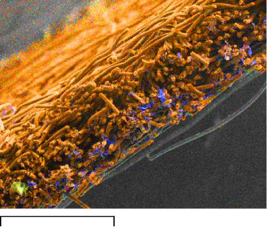
300 $\mu$m

Figure 2: Microscopic picture of the gas diffusion layer

Figure 2 shows that cross sections of fibers of gas diffusion layers are almost circular. There are also gas diffusion layers with a little variance in the fiber radii, although they are mostly nearly constant. Anyhow the variance of the fiber radii is of course limited, since it is impossible to produce fibers with an arbitrarily large radius.

We have to remark that from a practical point of view the optimization problem (12) is not well posed. For the construction of gas diffusion layers, mainly the intensity of the fibers $\lambda$ can be varied. Hence a practically relevant optimization should involve maximizing the volume fraction $p$ with respect to $\lambda$ as well. Since the latter problem is much more involved than the one discussed here, it would go beyond the scope of this paper.
Acknowledgements We would like to thank Werner Nagel, Rolf Schneider, Dietrich Stoyan, Wolfgang Weil, and anonymous referees for their useful comments which helped us to improve the paper. Furthermore, we are indebted to Christoph Hartnig and Werner Lehnert for discussions about fuel cells and for providing Figures 1 and 2.

References

• Ambartzumian (1990) Ambartzumian RV (1990) Factorization Calculus and Geometric Probability, Encyclopedia of Mathematics and Its Applications, vol 33. Cambridge University Press, Cambridge
• Berryman (1987) Berryman JG (1987) Relationship between specific surface area and spatial correlation functions for anisotropic porous media. J Math Phys 28:244–245
• Corte and Kallmes (1962) Corte H, Kallmes O (1962) Formation and structure of paper: Statistical geometry of a fiber network. Transactions 2nd Fundamental Research Symposium 1961, Oxford pp 13–46
• Davy (1978) Davy P (1978) Stereology — a statistical viewpoint. PhD thesis, Australian National University, Canberra
• Helfen et al (2003) Helfen L, Baumbach T, Schladitz K, Ohser J (2003) Determination of structural properties of light materials by three–dimensional synchrotron–radiation imaging and image analysis. G I T Imaging & Microscopy 4:55–57
• Hoffmann (2009) Hoffmann LM (2009) Mixed Measures of Convex Cylinders and Quermass Densities of Boolean Models. Acta Appl Math 105(2):141–156
• König and Schmidt (1991) König D, Schmidt V (1991) Zufällige Punktprozesse. Teubner, Stuttgart
• Manke et al (2007) Manke I, Hartnig C, Grünerbel M, Lehnert W, Kardjilov N, Haibel A, Hilger A, Banhart J (2007) Investigation of water evolution and transport in fuel cells with high resolution synchrotron X-ray radiography. Applied Physics Letters 90:174,105
• Matheron (1975) Matheron G (1975) Random Sets and Integral Geometry. J. Wiley & Sons, New York
• Mathias et al (2003) Mathias M, Roth J, Fleming J, Lehnert W (2003) Diffusion media materials and characterisation. Handbook of Fuel Cells III
• Molchanov et al (1993) Molchanov IS, Stoyan D, Fyodorov KM (1993) Directional analysis of planar fibre networks: Application to cardboard microstructure. J Microscopy 172:257–261
• Mukherjee and Wang (2006) Mukherjee PP, Wang CY (2006) Stochastic microstructure reconstruction and direct numerical simulation of the PEFC catalyst layer. Journal of the Electrochemical Society 153(5):A840–A849
• Ohser and Mücklich (2000) Ohser J, Mücklich F (2000) Statistical Analysis of Microstructures in Materials Science. J. Wiley & Sons, Chichester
• Schladitz et al (2006) Schladitz K, Peters S, Reinel-Bitzer D, Wiegmann A, Ohser J (2006) Design of acoustic trim based on geometric modelling and flow simulation for non–woven. Computational Materials Science 38(1):56–66
• Schneider (1987) Schneider R (1987) Geometric inequalities for Poisson processes of convex bodies and cylinders. Results in Mathematics 11:165–185
• Schneider (1993) Schneider R (1993) Convex Bodies. The Brunn–Minkowski Theory. Cambridge University Press, Cambridge
• Schneider and Weil (2008) Schneider R, Weil W (2008) Stochastic and Integral Geometry. Probability and Its Applications, Springer
• Serra (1982) Serra J (1982) Image Analysis and Mathematical Morphology. Academic Press, London
• Spodarev (2002) Spodarev E (2002) Cauchy–Kubota–type integral formulae for the generalized cosine transforms. Izv Akad Nauk Armen, Mat [J Contemp Math Anal, Armen Acad Sci] 37(1):47–64
• Stoyan et al (1995) Stoyan D, Kendall WS, Mecke J (1995) Stochastic Geometry and its Applications, 2nd edn. J. Wiley & Sons, Chichester
• Weil (1987) Weil W (1987) Point processes of cylinders, particles and flats. Acta Appl Math 9:103–136