DESY 10-077
HEPTOOLS 10-019
SFB/CPP-10-44
News on Ambre and CSectors

Abstract

Mellin-Barnes and sector decomposition methods are used to evaluate tensorial Feynman diagrams in the Euclidean kinematical region. Few software packages are shortly described and few examples demonstrate their use.

1 Introduction

Mellin-Barnes (MB) methods (see e.g. [1] and references therein) and sector decomposition (SD) methods (see e.g. [2] and references therein) are frequently used in theoretical high energy physics calculations. We will restrict ourselves here mainly to Feynman loop integrals in $d$ dimensions. There are nowadays public software packages which may help to automatize these calculations. On the MB Tools webpage [3] there are useful codes which realize: analytic continuations of Mellin-Barnes integrals – MB.m [4] and MBresolve.m [5]; parametric expansions of Mellin-Barnes integrals – expansion.m (author M. Czakon) and barnesroutines.m (author D. Kosower). For the creation of MB representations and later calls of other tools, AMBRE.m can be used [6, 7], which we describe here. AMBRE v1.x generates multiloop scalar [planar] and one-loop Feynman integrals. Here we extend the package to v2.0, which may treat also tensor [planar] structures. For the sector decomposition method, there are two public programs. FIESTA [8] and FIESTA2 [9] calculate scalar Feynman integrals with Mathematica, while Bogner/Weinzierl’s (BW) program [10] allows to calculate basic polynomials needed for the calculation of any Feynman integral with the c++ based computer algebra system Ginac [11]. Here we describe the Mathematica program CSectors.m which may serve as a kind of user interface to BW and Ginac in order to calculate fully automatically tensor Feynman integrals.

2 General tensor structure

We consider the $L$ loop Feynman momentum integrals with $N$ propagators $P_{n}$ and tensor structure $T(k)$:

$$G_{L}[T(k)]\equiv\frac{1}{(i\pi^{d/2})^{L}}\int\frac{d^{d}k_{1}\dots d^{d}k_{L}T(k)}{P_{1}\dots P_{N}}$$ (1)

$$= \frac{1}{(i\pi^{d/2})^{L}}\int\frac{d^{d}k_{1}\ldots d^{d}k_{L}~{}~{}T(k)}{(q_{1}^{2}-m_{1}^{2})^{\nu_{1}}\ldots(q_{N}^{2}-m_{N}^{2})^{\nu_{N}}}$$

$$= \frac{(-1)^{N_{\nu}}}{\Gamma(\nu_{1})\dots\Gamma(\nu_{N})}$$

$$\times~{}\int\prod_{j=1}^{N}dx_{j}x_{j}^{\nu_{j}-1}\delta\left(1-\sum_{i=1}^{N}x_{i}\right)$$

$$\times~{}\sum_{r\leq m}\frac{\Gamma\left(N_{\nu}-\frac{d}{2}L-\frac{r}{2}\right)}{(-2)^{\frac{r}{2}}}{{\frac{U^{N_{\nu}-\frac{d}{2}(L+1)-m}}{F^{N_{\nu}-\frac{d}{2}L-\frac{r}{2}}}}}$$

$$\times~{}{{\left\{{\cal A}_{r}P^{m-r}\right\}^{[\mu_{1},\ldots,\mu_{m}]}}}.$$

The momenta $q_{i}$ are linear combinations of internal momenta $k_{j}$ and external momenta $p_{n}$, and $T(k)$ is a tensor structure, e.g. ($1,k_{l}^{\mu},k_{l}^{\mu}k_{n}^{\nu},\ldots$). Further, $N_{\nu}=\sum\nu_{n}$. The general scalar $L$ loop integrals $G_{L}[1]$ are implemented in AMBRE.m v1.x, however tensor structures were allowed only for the one-loop case, $G_{1}[T(k)]$. The symbol $\{R\}^{[a_{1}\cdots a_{r}]}$ means the totally symmetrized sum of all possible combinations in the argument. We give as an explicit example the rank $R=3$ tensor:

$$\sum_{r\leq 3}\left\{{\cal A}_{r}P^{3-r}\right\}^{[\mu_{1}\mu_{2}\mu_{3}]}$$

$$= \left\{{{A_{0}}}P^{3}+{{A_{1}P^{2}}}+A_{2}P^{1}+{{A_{3}P^{0}}}\right\}^{[\mu_{1}\mu_{2}\mu_{3}]}$$

$$= P^{\mu_{1}}P^{\mu_{2}}P^{\mu_{3}}+\tilde{g}^{\mu_{1}\mu_{2}}P^{\mu_{3}}+\tilde{g}^{\mu_{2}\mu_{3}}P^{\mu_{1}}$$

$$+~{}\tilde{g}^{\mu_{3}\mu_{1}}P^{\mu_{2}}.$$

It is $A_{0}=P^{0}=1$, and $A_{r}$ is zero for $r$ odd, while ${\cal A}_{r}=\tilde{g}^{\left[\mu_{1}\mu_{2}\right.}\cdots\tilde{g}^{\left.\mu_{r-1}\mu_{r}\right]}$ for $r$ even. Further, $\tilde{g}^{\mu_{i}\mu_{j}}=(\tilde{M}^{-1})_{ab}g^{\mu_{i}\mu_{j}}$ and $P_{a}^{\mu_{i}}=\sum_{l}[\tilde{M}_{al}Q_{l}]^{\mu_{i}}$. The $\tilde{M}$ and $Q_{l}$ are defined from $\sum_{i=1}^{n}P_{i}x_{i}=\sum_{i=1}^{N}(q_{i}^{2}-m_{i}^{2})x_{i}=\sum_{i,j=1}^{L}k^{T}_{i}M_{ij}k_{j}-2\sum_{j=1}^{L}k^{T}_{j}Q_{j}+J$ and $\tilde{M}=\text{det}(M)M^{-1}$. The $U$ and $F$ polynomials were defined e.g. in [6, 7].

3 The package AMBRE.m

In [12] it is shown how the tensor structures introduced in section 2 lead, in the loop-by-loop approach, to a list of Mellin-Barnes representations. For that purpose, the following basic function of the AMBRE.m package is invoked:

MBrepr[{numerator},{propagators},
{internal momenta}].

Let us take the example of figure 1, and sketch a sample math file.

First, packages must be loaded:

<< MBv1.2.m

<< AMBRE.m

<< MBnum.m (3)

or

<< MBresolve.m (4)

<< barnesroutines.m

As indicated, barnesroutines.m works with version 1.2 of MB.m. If we want to use this package, the MB integrals up to the needed power in $\epsilon$ must be prepared first (by analytic continuation), and the second part of the sample MB_SE5l0m.m file may look as follows:

invariants = {p1^2 -> s};
repr = MBrepr[{k1*p1, k1*p1, k2*p1},
 {PR[k1,0,n1]*PR[k2,0,n2]*PR[k2-k1,0,n3]
 *PR[k1+p1,0,n4]*PR[k2+p1,0,n5]},
  {k2,k1}];

in the case of the MBnum.m package, followed by:

SetOptions[MBnum, Analytical -> True,
 Numerical -> False, ShowMBrep -> True];
MBanalytic = MBnum[repr, 1, {s -> -11},
 {n1->1, n2->1, n3->1, n4->1, n5->1}, 2];

or, in the case of the MBresolve.m package, followed by:

step1=MBresolve[#/.powers,eps]&/@repr;
step2=MBexpand[step1,
       Exp[2*eps*EulerGamma],{eps,0,1}];
MBanalytic=MBmerge[step2];

(6)

Finally, after getting the MB integrals at the $\epsilon$ level needed (here $\epsilon^{1}$, second argument of the MBnum function), we “Simplify” the result using Barnes lemmas with the internal MB.m functions MBmerge and MBintegrate:

after =
Process[MBanalytic, Range[10]]//MBmerge;
SEnumMB=MBintegrate[after,{s->-11}]

The phrase Range[10] means that we assume to get up to 10 dimensional MB representations; in fact, they are maximally 2-dimensional here.

The final result is:

$${\rm SEnumMB}=-7.5625/\epsilon^{2}-20.4506/\epsilon$$

$$-178.18\pm 0.0171936$$

$$+(18.3642\pm 0.0248465)\epsilon.$$ (7)

Singularities are here at most 1-dimensional integrals, so MB.m solves them within Mathematica very accurately and no error is given.

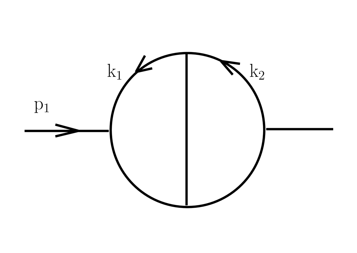
Figure 1: A 2-loop self energy topology.

4 The package CSectors.m

The package CSectors.m allows to derive integral representations for Feynman integrals, which are decomposed into so-called sectors with a well-defined singularity structure. The invariants should be of the Euclidean type. The structure of the main function is analogous to that in Ambre.m:

DoSectors[{numerator},{propagators},
{internal momenta}][low,des]

The sample executable file might look as follows:

#!/bin/bash
math << \FILE

<< CSectors.m

invariants = {p1^2->s}

SetOptions[DoSectors, SetStrategy -> C,
TextDisplay->True, SourceName->SE5l0m_num,
TempFileDelete->False];

max=0; s=-11;
invariants = {p1^2 -> s};

SEnumSD = DoSectors[{k1*p1,k1*p1,k2*p1},
 {PR[k1,0,1]*PR[k2,0,1]*PR[k2-k1,0,1]*
  PR[k1+p1,0,1]*PR[k2+p1,0,1]},{k2,k1}]
  [-2,max]

FILE

The numerical result in the example is (see also file SD_LL2010.out at [13]):

$${\rm SEnumSD}=-178.1927-7.56258/\varepsilon^{2}$$

$$-20.4505/\varepsilon+18.394000000000005\varepsilon,$$

$$\{0.011130644628528934,0.00029563/\varepsilon^{2},$$

$$0.00302109/\varepsilon,0.06629380324170578*\varepsilon\}.$$ (8)

The second bracket gives an error estimation. Due to the tensor structure (1), a number $A$ of integrals $I_{i}$ appear at a given $\epsilon$ level. An error for the numerical result $I_{\epsilon}$ at $\epsilon$ level is estimated in a standard way:

$$\Delta I_{\epsilon}=\sqrt{\sum_{i=1}^{A}(\Delta I_{i})^{2}}.$$ (9)

In the MB.m package the error $\Delta I$ is, for the single MB integral $I$, controlled by switching on an appropriate MB.m option: Debug->True. Let us just note that the error can be underestimated, see [4] and MB.m for details.

5 Mellin-Barnes approach versus Sector Decomposition approach

All the results given in the last section in (7) and (4) have been obtained with default parameters needed for numeric defined by the WB and MB.m packages. The total time of calculation on a Xeon PC with 32 GB RAM was in the MB case 17s and about 5 minutes for both the C- and X-strategies in the SD case.

Calculational times can differ substantially depending on methods and integrals. In table 1 and table 2, results for the massless and massive planar 2-loop topology B1 are given, see Fig. 2 and [14, 15] for the topology’s definition.

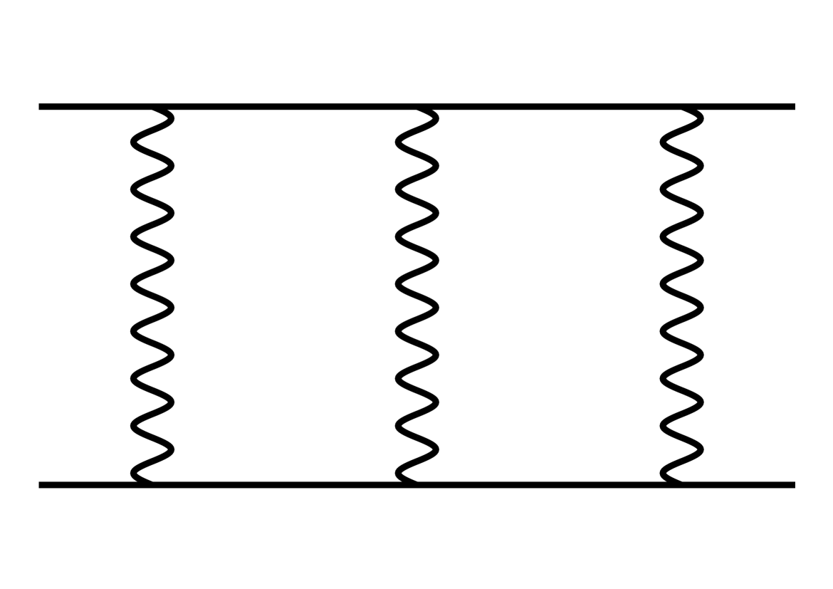
Figure 2: The planar 2-loop Bhabha topology B1.

Table 1: The scalar massless 2-loop planar double box $B1$, shown in figure 2. The scalar case allows for direct comparisons of the packages discussed here with FIESTA2. For source and output files see [7] and [13].

massless	AMBRE and MB
$\epsilon^{0}$	$-0.1034\pm 6\cdot 10^{-6}$
$\epsilon^{-1}$	$-0.10907$
$\epsilon^{-2}$	$-0.00966$
$\epsilon^{-3}$	$0.083188$
$\epsilon^{-4}$	$-0.022857$
T [s]	$22$
massless	CSectors, X-strat.
$\epsilon^{0}$	$-0.1035\pm 0.0002$
$\epsilon^{-1}$	$-0.10915\pm 0.00008$
$\epsilon^{-2}$	$-0.00966\pm 0.00001$
$\epsilon^{-3}$	$0.083191\pm 0.000005$
$\epsilon^{-4}$	$-0.0228574\pm 1\cdot 10^{-6}$
T [s]	$1712$
massless	FIESTA2
$\epsilon^{0}$	$0.103267\pm 0.001117$
$\epsilon^{-1}$	$0.109049\pm 0.000348$
$\epsilon^{-2}$	$0.009656\pm 0.000082$
$\epsilon^{-3}$	$-0.08319\pm 0.000012$
$\epsilon^{-4}$	0.022858
T [s]	$350$
$s=-5$, $t=-7$

Table 2: The scalar massive 2-loop planar double box $B1$.

massive	AMBRE and MB
$\epsilon^{0}$	$0.2246$
$\epsilon^{-1}$	$0.06359$
$\epsilon^{-2}$	$-0.023524$
T [s]	$42$
massive	CSectors, C-strat.
$\epsilon^{0}$	$0.2246\pm 0.0001$
$\epsilon^{-1}$	$0.06357\pm 0.00003$
$\epsilon^{-2}$	$-0.023524\pm 4\cdot 10^{-6}$
T [s]	$362$
massive	FIESTA2
$\epsilon^{0}$	$-0.224756\pm 0.000485$
$\epsilon^{-1}$	$-0.063622\pm 0.000102$
$\epsilon^{-2}$	$0.023528\pm 0.00001$
T [s]	$35$
$s=-5$, $t=-7$, $m=1$

We can see that in the case of the massless box B1, the MB method can be much faster than the SD method. In the massive case the difference is smaller, moreover, the SD method can be often faster. In addition results obtained by FIESTA2 [9] are presented. Note a difference in sign between FIESTA2 and MB/SD, see [9] for FIESTA2 conventions.

For completeness, the FIESTA2 sample Mathematica file for getting the numbers in Table 2 is reproduced:

<< FIESTA_2.0.0.m;
CIntegratePath="./CIntegrateMP"
QLinkPath = "./QLink64"

invariants =
{p1^2->m^2,p2^2->m^2,p3^2->m^2,p4^2->m^2,
 p1*p2->1/2*s-m^2,p3*p4->1/2*s-m^2,
 p1*p3->1/2*t-m^2,p2*p4->1/2*t-m^2,
 p2*p3->1/2*u-m^2,p1*p4->1/2*u-m^2}
 /.u->4*m^2-s-t/.m->1//Simplify;
kinematics = {s -> -5, t -> -7};

integral=PR[k1,1,n1]*PR[k1+p1,0,n2]*
 PR[k1+p1+p2,1,n3]*PR[k1-k2,0,n4]*
 PR[k2,1,n5]*PR[k2+p1+p2,1,n6]*
 PR[k2 + p1 + p2 + p4, 0, n7];
fintegral=(List @@ integral)
  /.PR[q_,m_,n_]->-(q^2-m^2);

SDEvaluate[UF[{k1,k2},fintegral,
        Join[invariants, kinematics]],
         {1,1,1,1,1,1,1},0]

6 Summary

The CSectors.m package has been prepared in order to allow an easy use of the SD package by Bogner/Weinzierl for the evaluation of Feynman tensor integrals. The AMBRE package has been enlarged to involve tensor structures for multiloop integrals in an automatic way. We are planning for the near future to automatize the construction of MB representations for nonplanar diagrams, what deserves not to use the loop-by loop approach. Further, we will foresee to build MB representations for special forms of linear propagators which are present e.g. in the HQET theory or in calculations of the QCD static potential (see the talk by V. Smirnov at this conference [16]).

References

- [1] V. A. Smirnov, Evaluating Feynman integrals, Springer Tracts Mod. Phys. 211 (2004) 1–244.
- [2] G. Heinrich, Sector Decomposition, Int. J. Mod. Phys. A23 (2008) 1457–1486. arXiv:0803.4177, doi:10.1142/S0217751X08040263.
-
[3]
MB Tools webpage
http://projects.hepforge.org/mbtools/ - [4] M. Czakon, Automatized analytic continuation of Mellin-Barnes integrals, Comput. Phys. Commun. 175 (2006) 559–571. arXiv:hep-ph/0511200.
- [5] A. V. Smirnov, V. A. Smirnov, On the Resolution of Singularities of Multiple Mellin- Barnes Integrals, Eur. Phys. J. C62 (2009) 445–449. arXiv:0901.0386, doi:10.1140/epjc/s10052-009-1039-6.
- [6] J. Gluza, K. Kajda, T. Riemann, AMBRE - a Mathematica package for the construction of Mellin-Barnes representations for Feynman integrals, Comput. Phys. Commun. 177 (2007) 879–893. arXiv:0704.2423[hep-ph].
- [7] Katowice webpage http://www.us.edu.pl/gluza/ambre, DESY webpage http://www-zeuthen.desy.de/theory/research/CAS.html.
- [8] A. Smirnov, M. Tentyukov, Feynman Integral Evaluation by a Sector decomposiTion Approach (FIESTA), Comput.Phys.Commun. 180 (2009) 735–746. arXiv:0807.4129, doi:10.1016/j.cpc.2008.11.006.
- [9] A. V. Smirnov, V. A. Smirnov, M. Tentyukov, FIESTA 2: parallelizeable multiloop numerical calculations. arXiv:0912.0158.
- [10] C. Bogner, S. Weinzierl, Resolution of singularities for multi-loop integrals, Comput. Phys. Commun. 178 (2008) 596–610. arXiv:0709.4092, doi:10.1016/j.cpc.2007.11.012.
- [11] C. W. Bauer, A. Frink, R. Kreckel, Introduction to the GiNaC framework for symbolic computation within the C++ programming language, J. Symbolic Computation 33 (2002) 1–12. arXiv:cs/0004015.
- [12] K. Kajda, et al., long write-up, in preparation.
- [13] Katowice webpage http://www.us.edu.pl/gluza/csectors, DESY webpage http://www-zeuthen.desy.de/theory/research/CAS.html.
- [14] M. Czakon, J. Gluza, T. Riemann, A complete set of scalar master integrals for massive 2- loop bhabha scattering: Where we are, Nucl. Phys. Proc. Suppl. 135 (2004) 83–87. arXiv:hep-ph/0406203.
- [15] M. Czakon, J. Gluza, T. Riemann, Master integrals for massive two-loop Bhabha scattering in QED, Phys. Rev. D71 (2005) 073009. arXiv:hep-ph/0412164.
- [16] A. Smirnov, A. Petukhov, The number of master integrals is finite, talk at LL2010. arXiv:1004.4199.