Phase transitions in cellular automata
for cargo transport and kinetically constrained traffic

Abstract

A probabilistic cellular automaton for cargo transport is presented that generalizes the totally asymmetric exclusion process with a defect from continuous time to parallel dynamics. It appears as an underlying principle in cellular automata for traffic flow with non-local jumps for the kinetic constraint to drive as fast as possible. The exactly solvable model shows a discontinuous phase transition between two regions with different cargo velocities.

1 Introduction

Non-equilibrium phase transitions can rarely be calculated exactly, i.e. without need of approximations or fits of numerical data. One paradigmatic system where this is possible is the totally asymmetric simple exclusion process (TASEP) (see [1] and references therein). The model is defined on a 1d discrete lattice with sites being either empty (holes) or occupied by a single particle. A randomly chosen particle moves to the right at rate $1$ provided that the site is empty. For open boundaries with particle input at rate $\alpha$ and output at rate $\beta$ this leads to three different phases: a low-density, a high-density and a maximum-current phase. For finite systems the process can be solved exactly by the matrix-product Ansatz (see [2] for a recent and exhaustive review) and the complete thermodynamic behavior that is relevant for understanding the phase diagram can be extracted from the asymptotics of this solution. On the ring the process has a uniform groundstate [1]. However the presence of a defect particle leads to a rich phase behavior [3]. In the defect TASEP usual particles move $10\rightarrow 01$ at rate $1$, the single defect particle moves itself forward $20\rightarrow 02$ at rate $\alpha$ and can be overtaken by usual particles $12\rightarrow 21$ with $\beta$ The solution is formally related to the open-boundary case. There is one shock phase and three phases where it behaves once like a particle, once like a hole and once like a second-class particle. The second-class particle case corresponds to $\alpha=\beta=1$. To the left the second-class particle looks like a hole (as seen from a particle) and to the right it looks like a particle (as seen from a hole). This case was studied in [4] since it can be used to study the shock in the TASEP on the infinite line with step-initial condition. The connection is that, due to its very special dynamics, the defect $2$ samples the random shock position on preferring configurations like $000021111$.
The defect TASEP can alternatively be understood as a cargo transport process: The defect is a usual particle carrying a cargo which can be handed over to a particle behind. See [5] for a different definition of cargo in the same context. These mechanisms play a fundamental role in the biology of intracellular transport. Processive motors like kinesin transport cargo over long distances [6]. The cargo can alternatively be interpreted as virus particles that use carrier particles in order to attain the interior of a cell, see [5] for further references.
The Nagel-Schreckenberg model [7] is often referred to as the minimal model for one-lane traffic-flow on a freeway. There it is essential to allow for faster and slower cars to get a realistic flow-density relation: cars can move up to $v_{max}$ sites per time step. Further all cars are updated simultaneously according to a parallel update and move independently with probability $p$. For $v_{\rm max}=1$ it is equivalent to the TASEP with parallel dynamics. The steady state on the ring shows nearest-neighbor correlations and has a simple pair-factorized form [8]. For open boundaries the matrix-product technique could be generalized to obtain the exact steady state [9, 10]. It can be interpreted as a pair-factorized state as on the ring modulated by a matrix-product state [11].
In this article we introduce a generalization of the cargo-transport process to discrete time with parallel updating and give its exact solution. Here we restrict ourselves to light cargo, i.e. the case where the speed of a particle is not lowered by the presence of cargo. This appears naturally in the steady state of a traffic cellular automaton [11]. We will see that non-local jump processes where particles drive as fast as possible can lead for non-deterministic hopping to a discontinuous phase transition on the ring.

2 The Cellular-Automaton Model and its Solution

Consider a periodic one-dimensional lattice with sites being either occupied by a particle (in state $\tau=1$) or empty ($\tau=0$). One of the particles carries a cargo to which we refer to as a defect ($\tau=2$). The particles are updated simultaneously and every particle (with or without cargo) moves forward with probability $p$. If the site behind it is occupied, the cargo carrying particle can independently give its cargo back at probability $\beta$. This simple dynamics is encoded in detail in the transitions

$$10 \rightarrow 01, \text{at rate }p,$$ (1)

$$020 \rightarrow x02, \text{at rate }p,$$ (2)

$$120 \rightarrow 210, \text{at rate }\beta(1-p),$$ (3)

$$\rightarrow 102, \text{at rate }(1-\beta)p,$$ (4)

$$\rightarrow 201, \text{at rate }\beta p,$$ (5)

$$121 \rightarrow 21x, \text{at rate }\beta,$$ (6)

with $x$ being either $0$ or $1$ indicating that the site can be either empty or occupied due to the parallel update. For example the evolution of the pattern $020$ can be affected by a particle to the left moving itself forward. This is quite a general scenario that might apply to biological intracellular cargo transport. The parallel update reflects highly active transport where many particles move at the same time.
For $\beta=0$ the cargo is attached to one special particle for all times and its dynamics is the same as for the other particles. This corresponds to the usual TASEP (with parallel update) and the single occupation $\tau=2$ can be replaced by $\tau=1$. The steady state for a lattice with $L+1$ sites (with one of them occupied by the defect) is

$$P(\tau_{1},\tau_{2},\dots,\tau_{L+1})=\prod\limits_{i=1}^{L+1}P(\{\tau_{i-1},\tau_{i}\}),$$ (7)

thus it factorizes [8] into symmetric two-site factors $P(\tau_{i-1}\tau_{i})\equiv P(\{\tau_{i-1},\tau_{i}\})$ with

$$P(00) = 1-\rho-J/p,$$ (8)

$$P(10) = J/p,$$ (9)

$$P(11) = \rho-J/p.$$ (10)

Here $J$ is the particle current

$$J(\rho)=\frac{1-\sqrt{1-4p\rho(1-\rho)}}{2}.$$ (11)

We found [11] that the steady state for $\beta>0$ can be calculated exactly too. Here (7) is generalized to

$$P(2,\tau_{1},\dots,\tau_{L}) \propto \tilde{f}(\tau_{1})f(\tau_{1}\tau_{2})\dots f(\tau_{L-1}\tau_{L})\tilde{f}(\tau_{L})$$ (12)

$$\times \langle W|\left[\prod\limits_{i\geq 1}\tau_{i}D+(1-\tau_{i})E\right]|V\rangle$$

This is a pair-factorized state (mainly the steady state for $\beta=0$) modulated by a matrix-product state. Up to the normalization this is very related to the TASEP with open boundaries [9, 11]. The vectors $\langle W|$ and $|V\rangle$ represent the defect and the matrices $D$ and $E$ represent particles and holes respectively. The operators obey the algebra

$$\langle W|EE = (1-p)\langle W|E,$$ (13)

$$\langle W|ED = (1-p)\left(\langle W|D+p\right),$$ (14)

$$DE = (1-p)\left[D+E+p\right],$$ (15)

$$D|V\rangle = \frac{p(1-\beta)}{\beta}|V\rangle,$$ (16)

for details see [11]. Note that the relations (15) and (16) are quadratic and the other relations are cubic. Accordingly the dynamical rules in (1-6) are quadratic (for $10$ and $12$) and cubic (for $20$) respectively. The thermodynamic particle current (11) obviously is unaffected by the cargo.
This steady state appears also in cellular-automaton models for traffic flow with non-local jumps under kinetic constraint. Consider the following process on a periodic one-dimensional lattice with sites being either occupied by one car (in state $\tau=1$) or empty ($\tau=0$). The update rules applied simultaneously to all cars ($\equiv$ particles) are

$$100 \rightarrow 001,\quad{\rm with}\;{\rm probability}\;p,$$

$$101 \rightarrow 01x,\quad{\rm with}\;{\rm probability}\;\beta,$$

where $x$ denotes either a particle or hole. The maximum velocity $v_{\rm max}$ thus is two sites per time step instead of one in the usual TASEP and the kinetic constraint is that cars can not drive at reduced speed 1 if they could move at maximum speed. This leads under the parallel dynamics to a non-local repulsion between cars, so that finally in the thermodynamic limit only even gaps ($0,2,4,\dots$ holes) have non-vanishing probability. Figure 1 a) shows schematically the allowed moves in a stationary configuration.

Figure 1: a) Allowed moves in a stationary configuration: only one odd gap between particles b) Equivalence of moves and according reduction of lattice units

For even number of holes the process is equivalent to the TASEP and for odd number of holes it is equivalent to the cargo-transport process. In this case a single hole in an environment of particles and hole pairs is formed that plays the role of cargo attached to varying particles. In figure 1 b) one sees that the particle movement of a single site is equivalent to backward movement of the $01$ position. The $01$ pair plays the role of the defect, having the characteristic ‘Janus face’, looking to the left like a hole and to the right like a particle. Usual holes are replaced by hole twins $00$. To be precise, the probabilities (8,9) would be rewritten here as $P(00)\equiv P(0000)$, $P(01)\equiv P(001)\equiv P(0001)$. In the following we restrict ourselves in the terminology to the cargo-transport process.

3 The Phase Diagram

There is a discontinuous phase transition at [11] the density

$$\rho_{c}=\frac{\beta(1-\beta)}{p-\beta^{2}}.$$ (17)

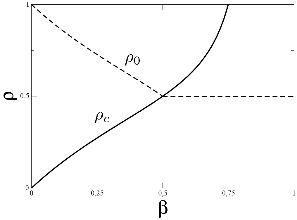
Figure 2: The phase diagram shows the $\rho$-$\beta$ plane for $p=3/4$. The thick line separates the two phases and on the dashed line the velocity of the defect changes its sign.

For $\rho<\rho_{c}$ and $\rho>\rho_{c}$ one finds different velocities of the defect which can be calculated through

$$v=p(1-\rho_{+})(1-\beta\rho_{-})-\beta\rho_{-}.$$ (18)

Here $\rho_{-}$ and $\rho_{+}$ are the densities directly behind and in front of the defect $2$. The dynamics of the defect is obtained from (1-6). It moves either forward with probability $p$ if it has a hole in front while at the same time there is no particle directly behind that simultaneously catches the cargo: first term in (18). Or it moves backwards with probability $\beta$ if it has a particle behind: second term in (18). The neighboring densities are in terms of the current $J(\rho)$ defined in (11):

$$\rho_{-}= \begin{cases}\dfrac{1}{\beta(1-\rho)^{2}}\dfrac{J^{2}(\rho-J)^{2}}{p(\rho-J)^{2}+(1-p)J^{2}},&\rm{for}\;\rho<\rho_{c},\\ \dfrac{p\rho-J}{p\rho-\beta J}&\rm{for}\;\rho>\rho_{c},\end{cases}\hfill$$ (19)

$$1-\rho_{+}= \begin{cases}\left(\dfrac{J}{p\rho}\right)^{2},&\rm{for}\;\rho<\rho_{c},\\ \dfrac{p-\beta}{p^{2}(1-\beta)}\dfrac{J}{\rho}&\rm{for}\;\rho>\rho_{c}.\end{cases}$$ (20)

Note that there are many ways to express the results due to the relation $J(1-J)=p\rho(1-\rho)$. In other words the square root in $J$ appears in every power of $J$ with a certain prefactor. Equations (19,20) yield

$$\frac{v(\rho)}{p}=\begin{cases}\dfrac{1-2\rho}{1-2J},&\rm{for}\;\rho<\rho_{c},\\ \dfrac{J-\beta\rho}{p\rho-\beta J}&\rm{for}\;\rho>\rho_{c}.\end{cases}$$ (21)

The defect velocity vanishes for

$$\rho_{0}=\begin{cases}\dfrac{p-\beta}{p-\beta^{2}},&{\rm for}\;\beta<1-\sqrt{1-p},\\ 1/2,&{\rm for}\;\beta>1-\sqrt{1-p},\end{cases}$$ (22)

and is positive for $\rho>\rho_{0}$ and negative for $\rho<\rho_{0}$. This leads to the phase diagram, depicted in figure 2.

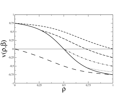
Figure 3: Velocity of the defect for $p=3/4$ for varying $\beta$. Continuous line: result for $\rho<\rho_{c}(\beta)$. The broken lines correspond to $\beta=0$, $\beta=0.25$, $\beta=0.5$, $\beta=0.67$ from top (dashed) to bottom (dotted) and are valid for $\rho>\rho_{c}(\beta)$. The segmented line is the velocity of holes

The formulae (17) and (22) can alternatively be interpreted in terms of a critical value $\beta_{c}\equiv\beta(\rho_{c})$ and $\beta_{0}\equiv\beta(\rho_{0})$. This gives

$$\beta_{c}=J(\rho_{c})/(1-\rho_{c}),\quad\beta_{0}=J(\rho_{c})/\rho_{c}.$$ (23)

The value of $\beta_{c}$ and $\beta_{0}$ respectively then is essentially the absolute velocity of holes and particles at the transition. Figure 3 shows the character of the defect and the discontinuous phase transition. For $\beta=0$ its velocity is given by the upper curve and equals the velocity of particles. In the zero-density limit the velocity is independently of $\beta$ equal to $p$. For increasing $\beta$ the second phase appears: The velocity of the defect jumps at $\rho=\rho_{c}(\beta)$ from the continuous curve to the corresponding dashed curve. $\rho_{c}$ increases with $\beta$ until $\beta=p$ where $\rho_{c}=1$, so that the system is completely in the second phase for all densities. Note that for $\beta=1/2$ one has $\rho_{c}=1/2$. Finally in the limit of the fully occupied lattice $\rho=1$ and $\rho_{c}\leq 1$ the velocity equals $\beta$ for $\beta\leq p$. However for $\rho_{c}>1$ it can never increase the value of $p$ which there is the corresponding velocity of the holes given by the segmented line.
For the phase $\rho<\rho_{c}$, which is purely present for $\beta\geq p$, it is important to stress that the quantities $\rho_{+}$, $\beta\rho_{-}$ and $v$ are independent of $\beta$. The density profile is symmetric around the defect and has an algebraic decay. This corresponds to the second-class particle phase in the defect TASEP mentioned in the introduction. As in continuous time the defect velocity (21) is given by $v=dJ/d\rho$ which has the form of a group velocity and becomes $v=1-2\rho$ for small $p$, compare table 1. Thus the defect travels with the velocity of the density disturbance.

4 Limits

Table (1) shows the limit of small hopping probabilities: $p\equiv dt$, $\beta=\tilde{\beta}dt$ with $dt\rightarrow 0$. Note in comparison that the velocity of normal particles is always $J/\rho$ which gives $p(1-\rho)+p^{2}(1-\rho)^{2}+\dots$ This limit has been studied in the traffic picture in [12, 13] and corresponds to the defect TASEP.

$\rho$	$v$	$1-\rho_{+}$	$\rho_{-}$
$\rho<\rho_{c}$	$(1-2\rho)dt$	$(1-\rho)^{2}\left[1+2\rho(1-\rho)dt\right]$	$\rho^{2}/\tilde{\beta}\left[1-(1-\rho)(1-3\rho)dt\right]$
$\rho>\rho_{c}$	$(1-\tilde{\beta}-\rho)dt$	$(1-\tilde{\beta})(1-\rho)\left[1+(\tilde{\beta}+\rho(1-\rho))dt\right]$	$\rho\left[1-(1-\rho)(1-\tilde{\beta}-\rho)dt\right]$

Table 1: Continuous-time limit $p\equiv dt$, $\beta\equiv\tilde{\beta}dt$: Values to the order $\mathcal{O}(dt)$ of velocity, empty-space density in front and particle density behind the defect in the two phases. Here $\rho_{c}\sim\beta\left[1-\beta(1-\beta)dt\right]$

As mentioned before, in the limit $\beta=0$ the defect moves only forward and loses its role as a defect. Therefore the steady state is the same as for the TASEP. Thus one has the expressions given in table (2).

$v$	$1-\rho_{+}$	$\rho_{-}$
$\;p\dfrac{P(10)}{\rho}=\dfrac{J}{\rho}\;$	$\;\dfrac{P(10)}{\rho}=\dfrac{J}{p\rho}\;$	$\;\dfrac{P(11)}{\rho}=1-\dfrac{J}{p\rho}\;$

Table 2: Limit of the discrete-time TASEP $\beta=0$

In comparison the results from (19,20,21) for $\rho>\rho_{c}$ are rewritten and expanded around the TASEP value:

$$\rho_{-}(\beta) = \frac{P(11)}{\rho-\beta P(10)}=\frac{P(11)}{\rho}\left[1+\frac{P(10)}{\rho}\beta+\dots\right]$$ (24)

$$1-\rho_{+}(\beta) = \frac{p-\beta}{p(1-\beta)}\frac{P(10)}{\rho}=\frac{P(10)}{\rho}\left[1-\frac{1-p}{p}\beta-\dots\right]$$ (25)

$$v(\beta) = \frac{J-\beta\rho}{\rho-\beta P(10)}=\frac{J}{\rho}-\left(1-\frac{J^{2}}{p\rho^{2}}\right)\beta-\dots$$ (26)

One sees that $\rho_{-}$ is mainly the same as for $\beta=0$ but the density to which the numerator is adressed is reduced by backward moving so that $\rho_{-}$ is increased. The same holds for the velocity $v$. $1-\rho_{+}$ is even the same as for $\beta=0$ up to a scale which is, using (17) and (22), given by $\rho_{c}/\rho_{0}$.
For $p=1$ (24)-(26) yield the results displayed in table 3.

$\rho$	$v$	$1-\rho_{+}$	$\rho_{-}$
$\rho<1/2$	$1$	$1$	$0$
$\rho>1/2$	$\dfrac{1-\rho-\beta\rho}{\rho-\beta(1-\rho)}$	$\dfrac{1-\rho}{\rho}$	$\dfrac{2\rho-1}{\rho-\beta(1-\rho)}$

Table 3: The partially deterministic case $p=1$: Velocity, empty-space density in front and particle density behind the defect.

For $\rho<1/2$ all particles are separated and move deterministically as in the TASEP. For $\rho>1/2$ the effect of $\beta$ on the velocity remains for all possible values and the phase transition disappears.

5 Conclusions

A cellular automaton for cargo transport was introduced that generalizes the (continuous-time) defect TASEP. The parallel update is often more realistic in describing active many-particle transport and makes the link between deterministic and random-sequential dynamics. The point of interest was a single defect, i.e. a particle carrying light cargo in an environment of particles and holes on a periodic 1d lattice. Particles move forward with probability $p$ and if a particle is directly behind the particle that carries the cargo it may catch the cargo with probability $\beta$. We found a discontinuous phase transition between two phases with different cargo velocities. Successively increasing $\beta$ lowers its velocity only until $\beta=p$. Then a saturation effect appears where the velocity becomes independent of $\beta$. The same holds for the stationary state of a cellular automaton for traffic where the ‘cargo’ corresponds to small headway that is formed dynamically. It is attached to one car from behind. If the subsequent car comes close enough it will catch it up. The fact that the cargo process appears in a seemingly unrelated non-local jump process underlines its universal role. The exact matrix-product state and its cubic algebra holds also for the two-species case where multiple cargo is present. It is also trivially generalized to case where cargo lowers the speed of the particle to $\alpha<p$. For $p=\beta$ and in the presence of several second-class particles it serves also as a model system for the study of shocks on the infinite line.

References

- [1] Derrida, B.: The asymmetric simple exclusion process: An exactly soluble nonequilibrium system. Phys. Rep. 301, 65 (1998)
- [2] Blythe, R.A., Evans, M.R.: Nonequilibrium steady states of matrix product form: A solver’s guide. J Phys. A 40, R333 (2007)
- [3] Mallick, K. Shocks in the asymmetry exclusion model with an impurity. J. Phys. A 29, 5375–5386 (1996)
- [4] Derrida, B., Janowsky, S.A., Lebowitz, J.L., Speer, E.R. Exact solution of the asymmetric exclusion process: Shock profiles. J. Stat. Phys. 73, 5/6, 813–843 (1993)
- [5] Goldman, C., Sena, E.: The dynamics of cargo driven by molecular motors in the context of asymmetric simple exclusion processes. Physica A 388, 3455–3464 (2009)
- [6] Korn, C., Klumpp, S., Lipowsky, R., Schwarz, U.S. Stochastic simulations of cargo transport by processive molecular motors. J. Chem. Phys. 131, 245107 (2009)
- [7] Nagel, K., Schreckenberg, M.: A cellular automaton model for freeway traffic.J. Phys. I France 2, 2221– 2229 (1992)
- [8] Schreckenberg, M., Schadschneider, A., Nagel, K. and Ito, N. Discrete stochastic models for traffic flow. Phys. Rev. E 51, 4, 2939–2949 (1995)
- [9] Evans, M.R., Rajewsky, N., Speer, E.R.: Exact solution of a cellular automaton for traffic. J. Stat. Phys. 95, 45–96 (1999)
- [10] de Gier, J. and Nienhuis, B.: Exact stationary state for an asymmetric exclusion process with fully parallel dynamics. Phys. Rev. E 59, 4899–4911 (1999)
- [11] Woelki, M. and Schreckenberg, M. Exact matrix-product states for parallel dynamics: Open boundaries and excess mass on the ring. J. Stat. Mech P05014 (2009)
- [12] Woelki, M., Schreckenberg, M.: Headway oscillations and phase transitions for diffusing particles with increased velocity. J. Phys. A 42, 325001 (2009)
- [13] Woelki, M. and Schreckenberg, M.: Phase transitions and even/odd effects in asymmetric exclusion models. In: Appert-Roland, C. et.al. (eds.) Traffic and Granular Flow 2007, pp. 435-440. Springer (2008)