Long duration gamma-ray bursts: hydrodynamic instabilities in collapsar disks

Abstract

We present 3D numerical simulations of the early evolution of long-duration gamma-ray bursts in the collapsar scenario. Starting from the core-collapse of a realistic progenitor model, we follow the formation and evolution of a central black hole and centrifugally balanced disk. The dense, hot accretion disk produces freely-escaping neutrinos and is hydrodynamically unstable to clumping and to forming non-axisymmetric ($m=1$, 2) modes. We show that these spiral structures, which form on dynamical timescales, can efficiently transfer angular momentum outward and can drive the high required accretion rates ($\geq 0.1-1~{}\textrm{M}_{\odot}~{}\textrm{s}^{-1}$) for producing a jet. We utilise the smoothed particle hydrodynamics code, Gadget-2, modified to implement relevant microphysics, such as cooling by neutrinos, a plausible treatment approximating the central object and relativistic effects. Finally, we discuss implications of this scenario as a source of energy to produce relativistically beamed $\gamma$-ray jets.

1 Introduction

Gamma-ray bursts (GRBs) were first reported by Klebesadel, Strong & Olson (1973) using data from the Vela satellites. The study consisted of 16 bursts lasting $\leq 30$ s, which were detected in an energy range of 0.2-1.5 MeV. Since then, the number of observed GRBs has risen into the thousands, using multiwavelength instruments, with burst durations spanning more than 5 orders of magnitude. Initial estimates of the total output of electromagnetic energy have been scaled down to $\approx 10^{50-52}~{}\rm{erg}$ with the assumption of relativistic beaming in jets. Observations to date of temporal duration and spectral hardness ratios confirm a bimodal distribution for the population: short duration bursts (SGRBs, $<2$ s) and long duration bursts (LGRBs, $>2$ s), with distinct progenitor scenarios assumed for each class. Here, we examine the latter with the aid of numerical simulations. In constructing realistic models, we first consider the observational constraints on progenitors and the microphysical processes which control the early phases of LGRB evolution and provide the required conditions for jet production.

A major breakthrough for the understanding of LGRBs came with their observed association with rather energetic Type Ic (core-collapse) supernovae (SNe), sometimes called hypernovae (HNe): first, with GRB980425 and SN1998bw (Galama et al., 1998), and then with GRB030329 and SN2003dh (Stanek et al., 2003). Properties of these and subsequent LGRB-SN associations are listed in Table 1. Studies of host galaxies have shown that LGRBs tend to occur in star forming regions (Le Floc’h et al., 2003), which may tend to have low-metallicity ($<0.3-0.5~{}Z_{\odot}$) (Fruchter et al., 2006). The emergent picture of the LGRB event is that of a massive (short-lived), stellar progenitor collapsing in on itself, which led to the adoption of the ‘collapsar’ model (Woosley, 1993) originally used in the context of core-collapse SNe.

Table 1: LGRB-HNe associations, with quantities calculated from observations (Pian et al., 2006; Mazzali et al., 2006; Nomoto et al., 2006; Valenti et al., 2008; Chornock et al., 2010; Starling et al., 2010).

GRB	Distance	$\textrm{T}_{90}$	$E_{\rm{iso}}$	SN	Bol. lum.	$M(^{56}$Ni)	$v_{\rm{max}}$
	($z_{\rm{est}}$)	(s)	($10^{50}$ erg)		($10^{42}$ erg s-1)	($\textrm{M}_{\odot}$)	($10^{3}$ km s-1)
980425	0.0085	34.9	0.01	1998bw	8.3	0.5-1.0	27
030329	0.169	22.8	180	2003dh	9.1	0.35	28
031203	0.105	37.0	0.26	2003lw†	11.0	0.55	18
100316D	0.059	$\sim$2300	$\geq 0.39$	2010bh	∗	∗	26
060218‡	0.033	$\sim$2100	0.62	2006aj	5.8	0.2	26
-	-	-	-	2003jd	5.6	0.3	$>$15

^† first observation 2 weeks after explosion;  ^‡ determined to be XRF;  ^∗ values unpublished, to date.

Briefly, the typical scenario begins with a rotating, massive star ($M/\textrm{M}_{\odot}>25-30$, possibly smaller if a remnant from a merger) collapsing to form a black hole (BH) from its core and a centrifugally-supported accretion disk, with continued infall from the surrounding stellar interior. The precise means of converting the energy of the disk material into high-energy photons and forming a relativistic jet is uncertain; however, the most studied methods, such as the Blandford-Znajek (B-Z) mechanism creating Poynting-flux (Blandford & Znajek, 1977; Lee, Wijers & Brown, 2000; Li, 2000) and neutrino annihilation accelerating plasma (Paczyński, 1990; Popham, Woosley & Fryer, 1999), require extreme and broadly similar conditions for the disk-BH system in order to reproduce observed GRB energies. In either case, accretion rates must be quite high, $\dot{M}_{\rm{acc}}\gtrsim 0.1-1.0~{}\textrm{M}_{\odot}~{}\textrm{s}^{-1}$. Structurally, the disk must be dense ($\rho>10^{8-10}~{}\textrm{g}~{}\textrm{cm}^{-3}$) and hot ($T\gtrsim 10^{10}~{}\rm{K}\sim 1~{}\rm{MeV}$), placing it in a regime where various scattering processes lead to large amounts of neutrino production. Most regions of these disks, while optically thick to electromagnetic radiation, are optically thin to neutrinos and therefore are able to cool quite efficiently; such disks are referred to as ‘neutrino-dominated accretion flows’ (NDAFs).

It is a great challenge for a physically realistic collapsar model to form such a disk (see discussion below in §2). The progenitor must possess enough specific angular momentum so that material will balance centrifugally outside of the BH innermost stable circular orbit (ISCO), which, for a moderately spinning 2-3 $\textrm{M}_{\odot}$ BH, is given by $j_{\rm{ISCO}}\geq 2-4\times 10^{16}~{}\textrm{cm}^{2}~{}\textrm{s}^{-1}$. It is then difficult to transfer that momentum outward efficiently to reach the required BH accretion rates. We note that some collapsar models have employed a rapidly rotating magnetar as a central engine (e.g. Usov, 1992; Thompson, 1994; Wheeler et al., 2000; Bucciantini et al., 2009), but we do not consider these alternative scenarios here.

Early studies treated NDAFs as thin disks using the Shakura-Sunyaev $\alpha$-viscosity ansatz to drive the accretion, for either steady state (Popham et al. 1999; Narayan, Piran & Kumar 2001; Kohri & Mineshige 2002) or time-dependent (Janiuk et al., 2004) solutions, typically assuming that the magneto-rotational instability (MRI) (Balbus & Hawley, 1991) could provide a physical mechanism for angular momentum transfer. A recent 2D study by Lopez-Camara, Lee & Ramirez-Ruiz (2009) with sophisticated equation of state (EoS) and cooling prescription found high accretion rates ($>0.1~{}\textrm{M}_{\odot}~{}\textrm{s}^{-1}$) and near-GRB neutrino luminosities ($\lesssim 10^{52}$ erg s^-1) for disks driven solely by the $\alpha$-viscosity, though (as presented here) the inclusion of azimuthal dynamics seems to be necessary to understand the full behaviour of collapsar flows. Ideal magneto-hydrodynamic (MHD) studies (Proga et al., 2003; Masada et al., 2007) have also produced high accretion rates, as have 2D numerical simulations studying viscosity-driven convection (for SGRB disks, Lee, Ramirez-Ruiz & Page, 2005); the creation of collapsar jets predominantly by the interplay of magnetic fields and neutrino annihilation has been investigated using 2D MHD and GRMHD (Nagataki et al., 2007; Nagataki, 2009). 3D simulations including general relativity have studied tori related to SGRBs producing high accretion and neutrino production rates (Setiawan, Ruffert & Janka, 2004; Shibata, Sekiguchi & Takahashi, 2007). However, the dominant physical processes during the evolution of a realistic, 3D collapsar system remains uncertain.

We consider the picture in which the hydrodynamic properties of a collapsar disk provide a mechanism for the high mass accretion rates giving rise to the LGRB. Since a BH formed from the iron core of a collapsed star has a mass of $\approx 2-3~{}\textrm{M}_{\odot}$, for a disk with sufficient mass to accrete at $0.1~{}\textrm{M}_{\odot}~{}\textrm{s}^{-1}$, the resulting disk/central object mass ratio, $\gtrsim 1/10$, is already quite large compared to most astrophysical systems. This ratio, combined with the high temperatures and densities mentioned earlier, has strong implications for the evolution of the system. Such self-gravitating disks are susceptible locally to clumping and are unstable globally to the formation of structures such as spiral arms, which are quite efficient at transferring angular momentum outwards and matter inwards. Moreover, neutrino production from the cooling material provides a possible mechanism for creating a jet from accelerated plasma, in addition to further destabilising such disks (Rice et al., 2003).

It is important to note that LGRBs exhibit a wide variety of characteristics in lightcurve shapes and afterglow spectra, as well as in associations with HNe (e.g., see discussion by Nomoto et al., 2007). To date, only four LGRBs have been linked with HNe (Table 1), while many partnerless ones have been seen at relatively close distances. Broadlined SNe Ic bright enough to be classified as HNe have been observed without LGRBs (Modjaz et al., 2008, and within); and at least one ‘HN’ has been associated with a less-energetic X-ray flash (XRF), XRF 060218-SN 2006aj (Campana et al., 2006). Certainly, viewing effects due to jet collimation play a role in some of the differences between events (Mazzali et al., 2005). For example, XRFs and unaccompanied HNe may be explained as LGRBs viewed slightly and greatly off-angle, respectively (the latter interpretation is supported by observed rates, e.g. Podsiadlowski et al., 2004).

It may be possible to explain much of this heterogeneity by considering the variation of a few physical factors among (qualitatively) similar progenitors: different values of rotation, core size or metallicity; varied circumstellar environments; etc. Certainly, LGRBs and related events have been observed across a wide range of epochs and environments. Assuming that (most) characteristics have reasonable ranges for permitting bursts, one would expect to have not only significant variation in burst behaviour but also the occurence of closely related, non-GRB events. For instance, systems with most (but not all) of the appropriate progenitor factors would likely yield ‘near-’ or imperfect LGRBs, i.e., producing weak or unobservable jets, or yielding sub-critical amounts of nucleosynthetic material for powering HNe. Complete understanding of LGRBs would include both mapping out the phase space of these factors, as well as determining properties of related phenomena by altering factors of successful events.

Here, we present a self-consistent model for powering LGRB engines via the collapsar mechanism using 3D numerical simulations. Starting with a physically realistic progenitor (from a stellar evolution code) soon after collapse, we follow the subsequent formation and evolution of an accretion disk around a compact object (a proto-neutron star (PNS) which accretes matter and becomes a BH). The aim of this study is to include as many as possible of the important microphysical and dynamical features of the system. Therefore, it has been necessary to use several approximations such as a simplified equation of state, appropriate for a radiation dominated polytrope; a time-independent estimation of electron fraction; and assumptions of nuclear statistical equilibrium (NSE), where appropriate, in determining constituent matter. To include effects of general relativity (GR) tractably, we first turn to standard pseudo-potentials with kinematic rescaling. We discuss the individual validity of these simplifications below. We note that, even while including several different types of physics, we generally find that the average estimated error for each approximation is $\lesssim$10-20%.

In §2, observational constraints on LGRBs are discussed, leading to our choice of progenitor and requirements of disk behaviour; in §3, we briefly introduce the numerical method used here, smoothed particle hydrodynamics (SPH); in §4, the further physics added to the SPH code are outlined, including a central object, relativistic effects, the calculation of electron fraction and constituent nuclei in the material, and cooling from neutrino production; in §5, the initial conditions of the various models are described; in §6-7, results of simulations with the shellular and cylindrical angular momentum profiles, respectively, are presented, with those of low temperature (shellular) models in §8; in §9, a test scenario with a simple jet is given; in §10, comparisons are made between models utilizing Newtonian and pseudo-Newtonian potentials; and finally, general trends and conclusions are discussed in §11.

2 Progenitor and Engine Requirements

In this section we review the broad constraints which LGRB observations and previously understood physics require from any physical collapsar progenitor. We also discuss how the success of any model is determined here, by judging the results of the formation and evolution of the disk-compact object system.

2.1 Observational and physical constraints

First, the progenitor must be massive, $M/\textrm{M}_{\odot}\geq 25-30$ for a single-star (Fryer, 1999), in order to form a BH from mainly core material. Also, a large supply of matter must be present, assuming that rapid accretion continues for most of the LGRB duration and that the event may be accompanied by a SN; e.g., an average accretion rate of $\dot{M}=0.5~{}\textrm{M}_{\odot}~{}\textrm{s}^{-1}$ for a 100 s burst would require 50 M_⊙, plus the mass of the SN ejecta as well. This progenitor range is in accordance with that of the large remnant mass ($\approx 3~{}\textrm{M}_{\odot}$) observed for SN 1998bw and the associated SN kinetic energies (related to the amount of radioactive nickel produced), $2-5\times 10^{52}~{}\rm{erg}$ (Nakamura et al., 2001). To date, all HNe associated with LGRBs have possessed broad-line spectral features, suggesting expansion velocities $\geq~{}20,000~{}\rm{km~{}s}^{-1}$ (e.g., see Pian et al. (2006) and references within).

Second, the LGRB-associated SNe were classified as Type Ic, due to the observed spectra containing neither H nor He lines. Therefore, it seems that, in general, the progenitor should possess no envelope at the time of collapse or, at least, one with only a very small amount of H and He. Furthermore, this lack of an envelope assists jet propagation near breakout from the star, greatly reducing the amount of radiation energy through dissipation into kinetic energy (avoiding the so-called ‘baryon mass-loading problem’).

In order to form a disk, a progenitor must be rotating rapidly, so that the entire star does not collapse directly into a BH. Instead, a large fraction becomes centrifugally balanced around a PNS/BH formed by the core, which in turn accretes material. Disk-BH systems are common in astrophysics (quasars, X-ray binaries, etc.) and tend to produce collimated outflows aligned along or near the rotation axis. Such systems are also typically very efficient in converting the energy of infalling matter into outgoing, beamed radiation. Any centrifugally supported disk must have enough specific angular momentum to remain outside of the BH $R_{\rm{ISCO}}$, noted before as $j\approx\rm{a~{}few}\,\times 10^{16}~{}\rm{cm^{2}~{}s^{-1}}$.

Finally, any collapsar disk must transport angular momentum outwards and mass inwards with great enough efficiency to produce the accretion rates required to power a GRB jet. In a study by Popham et al. (1999), most models required accretion rates of $\dot{M}>0.1~{}\textrm{M}_{\odot}~{}\textrm{s}^{-1}$ to produce a jet by B-Z or of $\dot{M}>0.1-1~{}\textrm{M}_{\odot}~{}\textrm{s}^{-1}$ for $\nu$-production and annihilation to produce luminosities $\gtrsim 10^{51}\textrm{erg}~{}\textrm{s}^{-1}$, although this depended on several factors such as BH spin, disk viscosity, etc. In the collapsar, a disk will be maintained by the continually infalling, high-$j$ stellar material which reaches centrifugal balance.

These few requirements are perhaps surprisingly difficult to combine within a self-consistent, robust model. As mentioned previously, during the evolution of the centrifugally formed disk, it becomes a formidable challenge to transfer angular momentum outwards efficiently enough to meet the necessary accretion rates. Similarly, difficulties arise in satisfying the characteristics of the progenitor itself; a massive star can easily lose its H/He envelope, but the typical mechanism of radiatively driven winds then causes the star to lose angular momentum efficiently as well (Langer, 1998; Langer, Heger & García-Segura, 1998).

Here, we address the latter difficulty by utilising a pre-collapse progenitor evolved from the merger of two helium stars (more details below in §5). The remnant object remains massive, while the merging process is able to eject outer envelope material from the system during a common-envelope phase (Podsiadlowski, Joss & Hsu, 1992). The polar direction is particularly cleared of H/He, benefitting jet propagation, and the remnant can easily retain sufficient angular momentum to form a centrifugally balanced disk. This is neither a very exotic nor overly restrictive requirement for the progenitor population, as at least half of all massive stars are estimated to be in binary and multi-star systems (Garmany, Conti & Massey, 1980; Kobulnicky & Fryer, 2007).

2.2 Disk evolution

We discuss here the dynamics controlling the evolution of the collapsar disk in different phases. First, after the initial collapse, viscous processes (along with neutrino cooling) determine transport and energy dissipation. Then, given the large self-gravity and the rapid cooling rate of the disk, we expect spiral arms to form on a dynamical timescale due to hydrodynamic instability. While viscous dissipation is still present in this latter phase, the spiral structure dominates the global transfer of angular momentum and leads to rapid accretion.

2.2.1 Disk viscosity

The evolution of thin and slim disks has been widely studied, typically in a low density regime but with an increasing interest in high density disks. Viscous processes in accretion disks convert kinetic energy to heat and transfer angular momentum outwards, though generally not at rates nearly as high as those required to drive LGRB production. Typically, this viscosity is attributed to the formation of convective currents, due to some combination of Maxwell (magnetic) and Reynolds (turbulent) stresses. Often in studies, these processes are parametrised as the $\alpha$ of Shakura & Sunyaev (1973), similar to an efficiency, which relates the overall viscosity to the local sound speed, $c_{\rm{s}}$, and scale height, $H$:

$$\nu=\alpha c_{\rm{s}}H\,.$$ (1)

Though a topic of some dispute, it is reasonable to assume that $\alpha\leq 1$, corresponding to a convection cell with size less than the disk height and with subsonic turnover.

Studies of Newtonian disks have shown that the presence of magnetic fields can lead to a magnetorotational instability (MRI), which induces efficient angular momentum transfer and dissipation (Balbus & Hawley, 1991), dominating disk dynamics with a maximal growth rate on the order of the dynamical timescale. This analysis assumes a Boussinesq (incompressible) flow, where the rotation profile is monotonically decreasing with radius, and that the plasma $\beta\geq 3$ (ratio of hydrostatic to magnetic pressure). Simulations using ideal (infinite conductivity) MHD have shown both axisymmetric and non-axisymmetric perturbations, leading to large accretion rates (Fromang, Balbus & De Villiers 2004; Fromang et al. 2004). In a physical disk, however, both the finite conductivity and resistivity of material can be important in damping the growth of the MRI, as discussed in Appendix A. We do not include any magnetic effects here, except by proxy through the influence of the $\alpha$-viscosity.

It has been shown that the numerical viscosity terms in SPH behave very similarly to a shearing viscosity in rotating systems. In the case of thin disks, (2D) studies have shown that the effective viscosity, $\nu_{\rm{SPH}}$, is proportional to the $\alpha$-viscosity (Murray, 1996; Taylor & Miller, in preparation). Therefore, the physical viscous process are essentially parametrised by the SPH viscosity.

2.2.2 Hydrodynamic instability

The Toomre parameter, $Q_{\rm{T}}$, (Safronov, 1960; Toomre, 1964; Goldreich & Lynden-Bell, 1965) has been used to characterise stability in several gaseous, stellar and hydrodynamic self-gravitating disk systems (e.g., Gammie, 2001; Rice et al., 2003). Moreover, it has been applied to describe both local stability against clumping and fragmentation, and the more global formation of spirals and non-axisymmetric modes. These structures can dramatically change the evolution of a disk. The Toomre parameter is given by

$$Q_{\rm{T}} = \frac{\kappa c_{\rm{s}}}{\pi G\Sigma}\,,$$ (2)

$$\kappa^{2} \equiv \frac{1}{R^{3}}\frac{d(\rm{a_{R}}\textit{R}^{3})}{dR}\,,$$

where $\kappa$ is the epicyclic frequency ($=\Omega$, orbital velocity, for Newtonian cases, and then often the stability parameter is approximated by $Q^{\prime}_{\rm{T}}=\Omega c_{\rm{s}}/\pi G\Sigma_{\rm{D}}$); $\rm{a_{R}}$, radial acceleration; $c_{\rm{s}}$, local sound speed; $G$, gravitational constant; and $\Sigma$, surface density of the disk. The exact critical value below which a disk is unstable to non-axisymmetric perturbations varies with the specific system but is usually $\approx 1$. For example, a finite-thickness, isothermal fluid disk has a critical value, $Q_{\rm{T}}\approx 0.676$ (Goldreich & Lynden-Bell, 1965; Gammie, 2001).

Physically, the Toomre parameter describes a competition between the locally stabilising influences of pressure, $P$ ($c_{\rm{s}}^{2}\propto T\propto P/\rho$), and epicyclic motion, and the destabilising influence of self gravity, which tends to enhance local clumpiness and global non-axisymmetry. From a global perspective, Hachisu, Tohline & Eriguchi (1987) have shown that (for cloud fragmentation) a parameter similar to $Q_{\rm{T}}$ can be derived by comparing relevant timescales in the system: the free-fall time, $\tau_{\rm{ff}}=(3\pi/32{\it G}\rho)^{\rm{1/2}}$; the sound crossing time, $\tau_{\rm{sd}}=2\pi{\it R}/c_{\rm{s}}$, for a cylinder of characteristic radius, $R$; and the epicyclic period, $\tau_{\rm{ep}}=2\pi/\kappa$. Besides identifying two stability criteria from the ratios $\tau_{\rm{ff}}/\tau_{\rm{sd}}$ and $\tau_{\rm{ff}}/\tau_{\rm{ep}}$, the product of these ratios is directly proportional to the Toomre parameter as given by Eq. 2 above, $Q_{\rm{T}}\propto\tau_{\rm{ff}}^{2}/\tau_{\rm{sd}}\tau_{\rm{ep}}$.

Studies of rotating polytropic disk models have suggested that $m=1$ and $m=2$ instabilities can develop on dynamical timescales (Imamura, Durisen & Pickett, 2000). There, angular momentum was transported outward in an initial pulse, followed by continued mass drain through the bar/spiral’s interaction with outer material.

Additionally, cooling plays a large role in the disk dynamics and evolution. Besides causing vertical contraction, the rate of cooling, $\dot{Q}^{-}$, has an important effect on the dynamical formation of non-axisymmetric structure. Simulations of both local and global stability (Gammie, 2001; Rice et al., 2003, respectively) showed that when the cooling timescale for a fluid element of specific internal energy, $\epsilon$, is of the order of the disk orbital period, i.e.

$$t_{\rm{cool}}\equiv\frac{\epsilon}{\dot{Q}^{-}}\approx\rm{a~{}few}\,\Omega^{-1},$$ (3)

then massive disks can rapidly become unstable to fragmentation and/or to non-axisymmetric structure formation on dynamical timescales.

One can think of this cooling effect entering into the Toomre criterion via thermal pressure and the $1^{\rm{st}}$ Law of Thermodynamics. If a fluid element in equilibrium is compressed without a cooling mechanism, then $P$ ($\propto\epsilon\rho$) increases, resisting compression and returning the volume to equilibrium. If the same element is compressed in the presence of a cooling mechanism, the internal energy necessarily increases less (or decreases), and $P$ cannot restore the same equilibrium. In some cases, these local overdensities propagate as spirals, becoming global modes.

While useful predictions of disk stability can be made from these analytic arguments, the resulting phenomena are highly nonlinear. Furthermore, in the collapsar case the further effects of relativistic dynamics (on both the epicyclic frequency and the disk structure) are uncertain. Therefore, any discussion of disk behaviour and evolution in the presence of non-axisymmetric perturbations requires 3D numerical modelling for a range of initial conditions.

2.3 Energetic requirements

The full details of the process of producing a relativistically beamed GRB jet are uncertain, and in this study we do not select one of the several proposed mechanisms. Here, we discuss the necessary conditions given by analytic arguments for disk-BH evolution in both the Blandford-Znajek (B-Z) and neutrino annihilation scenarios, which currently are the leading jet mechanisms and have been widely studied. The very complicated LGRB central engine and process of jet formation are thus characterised in terms of a few measurable, ‘physical’ quantities of the evolving system, which is obviously a great simplification and relies on many assumptions for each model. In the current field of LGRB studies, these approximations serve as the best evaluation for a collapsar system to produce a burst, but they can neither preclude new mechanisms nor definitively describe the full behaviour of an individual one.

In the B-Z mechanism, rotational energy of the disk-BH system is converted into Poynting-flux jets along the rotation axis. In addition to the BH spin and mass accretion rates, the flux of the outflow depends on the strength of a central magnetic (dipole) field which reaches outward from the BH. For a $3~{}\textrm{M}_{\odot}$ BH with a $10^{15}$ G magnetic field, the jet energy is given as a function of BH spin, $a$ ($\equiv Jc/GM^{2}$, the ratio of total BH specific angular momentum to mass), and accretion rate, $\dot{M}$, as (Thorne, Price & MacDonald, 1986):

$$\dot{E}_{\rm{B-Z}}\approx 3\times 10^{52}\,a^{2}\,\left(\frac{\dot{M}}{\textrm{M}_{\odot}~{}\textrm{s}^{-1}}\right)~{}~{}~{}\rm{erg~{}s^{-1}}.$$ (4)

In the case of neutrino annihilation, disk models studied by Popham et al. (1999) only reached GRB-like luminosities of $\gtrsim 10^{51}~{}\rm{erg~{}s^{-1}}$ with accretion rates of $\approx 0.1~{}\textrm{M}_{\odot}~{}\textrm{s}^{-1}$ and a few$\,\times\,0.1~{}\textrm{M}_{\odot}~{}\textrm{s}^{-1}$ for $a=0.95$ and 0.5, respectively. Neutrino production varied greatly with BH spin and disk viscosity, and in general, estimations to translate $L_{\nu}$ directly into jet energy remain quite uncertain. The efficiency of neutrino annihilation in plasma is unknown, particularly in the presence of other physical factors such as magnetic fields, baryon pollution, etc. Analysing idealised disks around Kerr BHs using ray-tracing techniques, Birkl et al. (2007) estimated the effects of both GR and disk geometry on neutrino annihilation rates. In general the effects were small (most less than a factor of 2), with more efficient annihilation associated with thinner disks and higher BH spins. For this study, we note in particular the important influence of the latter, as the smaller $R_{\rm{ISCO}}$ with increased $a$ leads to greater $L_{\nu}$ in the inner regions as well.

The neutrino case can be generalised more broadly with the simple assumption (e.g., Janka et al., 1999) that the useable neutrino energy rate for producing a LGRB jet, $\dot{E}_{\nu}$, scales directly with the total disk $L_{\nu}$:

$$\dot{E}_{\nu}=\eta_{\nu\bar{\nu}}L_{\nu}\,,$$ (5)

where $\eta_{\nu\bar{\nu}}$ now represents the total, unknown efficiency for the physical process of neutrino annihilation. This is a very uncertain quantity, and studies have shown that this efficiency may not be constant. Here, we will consider it to have a reasonably high value, $\eta_{\nu\bar{\nu}}=0.01$, as found by Janka et al. (1999) (see also, Ruffert & Janka, 1998), accepting that this is a very rough approximation.

In this study $\dot{E}_{\rm{GRB}}=10^{51}~{}{\rm erg~{}s^{-1}}\equiv 1~{}\textrm{foe}~{}\textrm{s}^{-1}$ is defined as our fiducial LGRB-jet energy flux, the threshold value which a successful central engine must produce. This value is generally consistent with observed LGRB energetics and would then require, for a BH with $a=0.5$, for example, an accretion rate of $\dot{M}>0.13~{}\textrm{M}_{\odot}~{}\textrm{s}^{-1}$ in the case of the B-Z mechanism. However, we do not intend this to preclude the possibility of lower-luminosity bursts which, as of this time, have not been detected (see discussion in Chapman, Priddey & Tanvir, 2009). In fact, such objects or ‘failed’ LGRBs may produce other observed phenomena, such as polarised SNe, XRFs, etc., particularly in the presence of a large central $B$-field.

3 SPH

For this study we use smoothed particle hydrodynamics (SPH) (Gingold & Monaghan, 1977; Lucy, 1977), which has found wide usage in modeling various astrophysical phenomena. SPH has advantages over other numerical techniques in that it naturally adapts to following dynamic flows and arbitrary geometries without the need for mesh refinement or other readjustment techniques required in Eulerian-based codes. The Lagrangian method allows natural definitions for the energetics of fluid elements and also efficiently maps structures whose density spans several orders of magnitude. We utilise the public release version of the Gadget-2 code (Springel, 2005), which, furthermore, strictly conserves momentum (linear and angular), energy and entropy. We add additional relevant physics to the code, such as cooling, relativistic effects and the presence of a central object.

Briefly, in SPH a continuous fluid is sampled at a finite number of points, and discretised versions of the three hydrodynamic equations (mass, momentum and energy) are calculated. Gadget-2 utilises a polytropic EoS and, rather than energy, evolves an entropic function, $K(s)=P/\rho^{\gamma}$, where $\gamma$ is the usual adiabatic index; $P$ and $\rho$, the hydrodynamic pressure and density, respectively, related to specific internal energy, $\epsilon=(\gamma-1)P/\rho$; and $s$ is specific entropy. The smoothed kernels determine a set of nearest neighbours which interact with symmetric hydrodynamic forces. Entropy is created from discontinuities and shocks, via a viscosity formulation which possesses two terms. The first provides the bulk and shear viscosity (linear in converging velocity), and the second, an artificial von Neumann-Richtmyer (quadratic) viscosity, mimics naturally dissipative processes in addition to preventing interparticle penetration (Monaghan, 1997). The strength of the Gadget-2 viscosity is parametrised by a single coefficient of order unity (here, $\alpha_{\rm v}=0.8$), and the Balsara prescription to reduce numerical viscosity introduced in rotating flows was utilized (Balsara, 1995; Steinmetz, 1996). Density is not explicitly evolved but instead is recalculated at each timestep from a weighted average of the total mass within a smoothed kernel. Gravitational forces are calculated efficiently with a hierarchical multipole expansion, using standard tree algorithms (e.g. Barnes & Hut, 1986).

4 Additional Physics

To these general hydrodynamic and gravitational components, we include physical features specifically relevant to the collapsar evolution. Unless otherwise stated, all temperatures, $T$, are given in units of K, and both mass and proton density, $\rho$ and $Y_{\rm{e}}\rho$, respectively, in units of $\textrm{g}~{}\textrm{cm}^{-3}$.

4.1 Central object

After collapse, the iron core of the initial progenitor first forms a (rotating) PNS, which subsequently accretes material to become a BH. Since our main concern is studying the behaviour of the accretion flow, we focus on simulating only the main effects of each distinct phase on the hydro-flow. The two most important influences of the central object are to provide an inner accretion boundary for the inflowing material and to exert gravitational accelerations (see §4.2 below, regarding relativity). Here, we discuss how the PNS and BH differ importantly in the presence and absence, respectively, of a surface pressure.

In the first few seconds after formation, the central object is quite hot and is best described as a PNS, with slightly larger radius than the typical 10-12 km of a NS, as well as a ‘softer’ surface. As the PNS accretes matter, its radius decreases, and we approximate its mass-radius (M-R) progression using the recent calculations of Nicotra (2006). Examples (using baryonic mass) of ($M_{\rm{PNS}}/\textrm{M}_{\odot}$, $R_{\rm{PNS}}/{\rm{km}}$) from his model T30Y04 are: (1.6, 35), (1.7, 24) and (1.9, 16), beyond which a BH is formed.

To approximate the surface of a (spherical) PNS, we include a radially-outward acceleration at the given $R_{\rm{PNS}}$, which interacts with SPH particles that have approached to within a fraction of their smoothing-length. For inflowing material, we add into the particle’s Euler equation an acceleration term which mimics the steep pressure gradient of the outer PNS, $a_{\rm{R}}=-\nabla P/\rho$, approximated from the Tolman-Oppenheimer-Volkoff (TOV) equation for our model. However, fluid elements with density greater than that at neutron drip ($\rho>\rho_{\rm{drip}}=4\times 10^{11}\textrm{g}~{}\textrm{cm}^{-3}$) accrete directly. The important aspect in these specifics is to provide a reasonable representation of the PNS effects on the evolving disk material, and we do not expect a strong model-dependence from using these relations.

A fluid particle accretes onto the central object in two ways. Most basically, when it reaches $R_{\rm{PNS}}$ with specific angular momentum, $j$, then the particle’s mass, $m$, and total angular momentum about the axis of rotation, $J=mj$, are added to that of the PNS (calculating $j$ is further discussed in §4.2). Also, since SPH particles represent a density distributed through a kernel, we ‘accrete’ a fraction of the mass, $m_{\rm{f}}$, and total angular momentum, $J=m_{\rm{f}}j$, as the particle approaches $R_{\rm{PNS}}$ to within a fraction of the smoothing length. This action also requires that any accreting particle’s smoothing length must be much less than $R_{\rm{PNS}}$, effectively establishing a resolution requirement for the simulation.

Above its maximum mass, the PNS becomes a BH, whose properties are determined, in this case, solely by its mass and spin. During this stage, the flow boundary possesses no surface pressure and is approximated as the surface of a sphere with radius $r_{\rm{in}}=R_{\rm{ISCO}}$ of a Kerr BH in the equatorial plane. All matter is co-rotating with the BH, and $r_{\rm{in}}$ can be calculated exactly (Novikov & Frolov, 1989, and see Eq. (7), below). The numerical procedure of the accretion is the same as in the PNS case, and we note that the final $R_{\rm{PNS}}$ is fortuitously similar to $r_{\rm{in}}$ for a newly-formed BH, which prevents the introduction of numerical errors at the conversion.

4.2 General and special relativity

In order to include effects of general relativity in an approximate manner, we add the acceleration of a pseudo-Newtonian potential for the central object to the gravity calculated between the SPH particles, in both the BH and PNS phases; though, the effects are larger for the BH case due to its larger mass and greater spin, and also $R_{\rm{PNS}}>r_{\rm{in}}$ for all masses, so that the innermost flow is at a larger radius, further decreasing PNS-GR effects. In this section we utilise relativistic units with $c=G=1$, and, while the same treatment of acceleration is used for both types of compact object, below we refer to them collectively as ‘BH’.

Due to the large angular momentum of the accreted material, one must utilise approximations appropriate for a rotating central object. From the many pseudo-potenials which have been developed in different studies, we have chosen to use the form of inward radial free-fall acceleration, $\rm{a_{R}}(\textit{R})$, for a Kerr BH with mass, $M$, and specific angular momentum, $a$, given by Mukhopadhyay & Misra (2003):

$$\rm{a_{SEP}}(\textit{R})=\frac{\textit{M}}{\textit{R}^{2}}\left[1-\left(\frac{\textit{r}_{\rm{in}}}{\textit{R}}\right)+\left(\frac{\textit{r}_{\rm{in}}}{\textit{R}}\right)^{2}\right],$$ (6)

derived from what they call the ‘Second-order Expansion Potential’ (SEP), where all radii have been scaled to gravitational units, $r_{\rm{g}}=GM/c^{2}$, and $r_{\rm{in}}$ is the location of the ISCO, given by:

$$r_{\rm{in}} = 3+Z_{2}-[(3-Z_{1})(3+Z_{1}+2Z_{2})]^{1/2}\,,$$ (7)

$$Z_{1} = 1+(1-a^{2})^{1/3}[(1+a)^{1/3}+(1-a)^{1/3}]\,,$$

$$Z_{2} = (3a^{2}+Z_{1}^{2})^{1/2}\,.$$

We discuss this choice of pseudo-potential and compare its characteristics to others, as well as to full GR solutions, in Appendix B.

In order to keep track of the BH spin parameter, $a$, we add to it the total angular momentum of all accreted material, $J=mj$. For material accreting from the equatorial plane, we approximate the specific angular momentum, $j$, as that of a corotating particle in circular orbit at $r_{\rm{in}}$, given as (Shapiro & Teukolsky, 1983):

$$j_{\rm{K}}=\sqrt{\frac{M}{r_{\rm{in}}}}\frac{(r_{\rm{in}}^{2}-2a\sqrt{Mr_{\rm{in}}}+a^{2})}{(r_{\rm{in}}^{2}-3Mr_{\rm{in}}+2a\sqrt{Mr_{\rm{in}}})^{1/2}}\,,$$ (8)

which is a several times larger than the Newtonian equivalent in the vicinity of the accretion boundary. In the case of polar accretion (defined as when the distance to the equatorial plane is greater than that to the rotation axis), we simply use the Newtonian value, $j=xv_{\rm{y}}-yv_{\rm{x}}$. Necessarily, this material will tend to have much less angular momentum anyway, so that this is a reasonable approximation.

For all velocities discussed here, we utilise a simple special-relativistic rescaling of the values occuring within the pseudo-potential, $v_{\rm{ps}}$:

$$v_{\rm{SR}}=\frac{v_{\rm{ps}}}{\sqrt{1+v^{2}_{\rm{ps}}}}\,.$$ (9)

This has been shown by Abramowicz et al. (1996) to produce velocities within 5% of relativistic calculations around non-rotating BHs when used in conjunction with the Paczyński-Wiita potential (Paczyński & Wiita, 1980).

We recognize that using these approximations to the Kerr metric in order to represent the gravitational contribution of the central object is a rough way of proceeding, but we believe that it constitutes a legitimate approach at the present stage of the work (see further discussion in Appendix B). In the case where the central object is a BH, it is clearly very approximate to treat the gravitational acceleration on fluid elements as the sum of contributions of a vacuum BH pseudo-potential and the Newtonian self-gravity of surrounding matter. In the case where the central object is a PNS, the surrounding spacetime differs from that of the Kerr metric anyway, with the former having quadrupole moments considerably larger than those for equivalent BHs. (However, it must be noted that the effect of the quadrupole falls off as $R^{3}$, so the influence of this difference for the disk flow may not be very great.) Improving on this treatment remains a topic for future work, but we believe that the approach being used here is a reasonable one at present.

4.3 Neutrino cooling

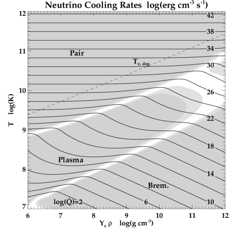
Figure 1: Solid lines show contours of the total combined cooling rate, $\dot{Q}_{\nu}$. The dark shaded regions show where a single production process dominates $>90\%$ of the total cooling rate, and the lighter, $>75\%$. Included for reference is the electron degeneracy temperature, T_e,deg.

In the inner regions of the collapsing star, the flow is optically thick to electromagnetic radiation, so that radiative transfer is very inefficient and the energy carried away by photons is negligible. Instead, much of the material, particularly in the disk itself, occupies a region of ($Y_{\rm{e}}\rho,~{}T$) phase space where cooling via neutrino emission is important (calculating $Y_{\rm{e}}$ is discussed in the next section). In the collapsar system local neutrino production greatly influences disk stability, and, summed globally, it may provide a mechanism for relativistic jet production.

For the regions which are optically thin to neutrinos, energy from processes such as pair annihilation, plasmon decay and (non-degenerate) bremsstrahlung is carried away freely. Very dense regions with $\rho>5\times 10^{12}$ are considered to be optically thick to neutrinos, and using the common ‘lightbulb approximation’, cooling shuts off.

For the ranges $7\leq\log({\textit{T}})\leq 12$ and $6\leq\log(Y_{\rm{e}}\rho)\leq 12$, we utilise tables of data from detailed calculations by Haft, Raffelt & Weiss (1994) for the plasma processes and by Itoh et al. (1996) for pair annihilation; for non-degenerate bremsstrahlung scattering, we use the analytic approximation given by Hannestad & Raffelt (1998), $\dot{Q}_{\rm{Br}}=1.5\times 10^{33}\,T_{11}^{5.5}\,\rho_{13}^{2}~{}\rm{erg}~{}\rm{cm}^{-3}~{}\rm{s}^{-1}$, with the notation $T_{11}=T/10^{11}$, etc. Fig. 1 shows contours of the combined rates of neutrino cooling, $\dot{Q}_{\nu}$, with shaded regions where each process dominates total cooling. During the evolution of the collapsar disk, we note that nearly all material for which cooling is relevant occupies ($Y_{\rm{e}}\rho,~{}T$) states dominated by plasma processes and pair production.

The importance of the relations between various timescales for the stability of the collapsar disk has already been introduced in §2.2.2 (and $\tau_{\rm{NSE}}$ is discussed in §4.5). Fig. 2 shows the relevant cooling timescales ($t_{\rm{cool}}=\epsilon/\dot{Q}_{\nu}$) for neutrino processes in this phase space. Typical values of the dynamical timescale ($t_{\rm{dyn}}=\Omega^{-1}$, orbital period) around a 3 M_⊙, $a=0.5$ BH at different radii have also been calculated. For direct comparison, the dynamical timescales are overlaid on the phase space, with reference to the cooling-stability criterion of Eq. (3). Fluid at a given radius is stable against clumping for the various ($Y_{\rm{e}}\rho,~{}T$) states in the region below the $t_{\rm{dyn}}({\it r})$ contour, and unstable for those a few times above.

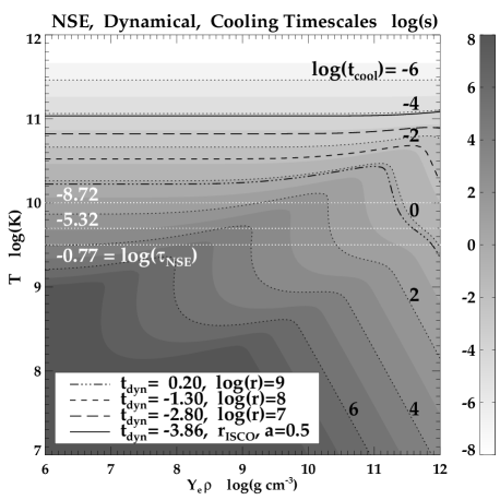
Figure 2: A comparison of timescales: the black (white) dotted lines show contours of $t_{\rm{cool}}$ ($\tau_{\rm{NSE}}$), from Eq. (3). In most regions $\tau_{\rm{NSE}}\ll t_{\rm{cool}}$. Values of dynamical timescale, $t_{\rm{dyn}}=\Omega^{-1}$, are given and overplotted on the $t_{\rm{cool}}$ contours for direct comparison regarding local stability.

4.4 Electron fraction

As the density of matter increases, so does the rate of capture of electrons by nuclei. This neutronisation decreases the electron fraction, $Y_{\rm{e}}$, and necessarily the proton/neutron ratio, below $0.5$. This change has important consequences for nuclear processes and cooling via neutrino production, which are dependent on the proton density, $Y_{\rm{e}}\rho$. For densities $\rho>10^{7}$, we follow the simple prescription of Liebendörfer (2005), who noted in core-collapse simulations that $Y_{\rm{e}}$ remains nearly constant in time and temperature for a given density. Using their ‘G15’ set of parameters, the approximate electron fraction, $Y_{\rm{e}}(\rho)$ is given by:

$$Y_{\rm{e}}(\textit{x}) = 0.354-0.111x$$

$$+\,0.035|x|\,[1+4\,(|x|-0.5)(|x|-1)]\,,$$

$$x(\rho) = \max\left[-1,\min\left(1,0.3434\,\log(\rho)-3.5677\right)\right]\,.$$ (10)

The electron fraction for a range of densities is shown by the vertical lines in Fig. 3. Thus, roughly-speaking, the electron fraction remains both temperature- and time-independent, with the restriction that, for a given $i$th fluid element, $Y_{\rm{e},{\it i}}$ monotonically decreases over time, i.e., upwards fluctuations are not permitted. Matter with density $\rho<10^{7}$ retains its initial value of $Y_{\rm{e},{\it i}}$.

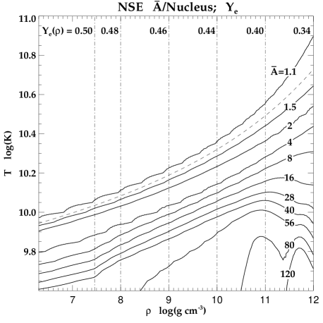
Figure 3: Contours show the average nucleon number, $\bar{A}$, in NSE for a given temperature and density, as calculated by F. Timmes (private communication). The dashed curve shows the commonly used onset of free nucleon matter. Vertical dot-dashed lines show density-dependent electron fraction, $Y_{\rm{e}}$.

4.5 NSE

In regions of high temperature and density, nuclear reactions involving strong interactions equilibrate with their inverse reactions, and nuclear statistical equilibrium (NSE) is reached (e.g., Hix & Meyer, 2006, and within). Assuming that matter remains transparent to neutrinos, element/isotope abundances may then be calculated using statistical relations which involve a large network of relevant isotopes, for material with $T\geq T_{\rm{NSE}}$ ($\equiv 4\times 10^{9}~{}\rm{K}\approx 0.34$ MeV). Importantly, in these regions Fe-group elements are formed, predominantly from Si-group elements created during a lower $(\rho,T)$, quasi-static equilibrium phase (QSE, e.g. Bodansky, Clayton & Fowler, 1968; Meyer, Krishnan & Clayton, 1998).

For calculating the average nucleon number, $\bar{A}_{\rm{NSE}}$, of a fluid element during the simulation, we consider matter with both $T>T_{\rm{NSE}}$ and $\rho>10^{6}$ to be in NSE (for a discussion of $\tau_{\rm{NSE}}$, see below). Computationally, a fluid element below $T_{\rm{NSE}}$ retains its pre-collapse $\bar{A}$ value. Knowing ($\rho,~{}Y_{\rm{e}},~{}T$), $\bar{A}_{\rm{NSE}}$ is determined from a table of values calculated by F. Timmes (private communication, and see Timmes, 1999) and shown as a function of temperature and density (as above, $Y_{\rm{e}}=Y_{\rm{e}}(\rho)$) in Fig. 3. Also shown as a guide is the often-used approximation for where the mass fraction of free neutrons and protons in material is unity, $X_{\rm{nuc}}=1$ (Woosley & Baron, 1992).

We calculate the abundances of specific $\alpha$- and heavy-elements produced by NSE conditions in the inner regions of the collapsar using results of the same reaction network calculations by F. Timmes (see Appendix C). Due to the observational association of LGRBs with HNe/SNe, we investigate in particular the production of ⁵⁶Ni, the radioactive isotope which is the dominant energy source of SN lightcurves via decay to ⁵⁶Co. A typical core collapse SN contains ${}^{56}\rm{Ni}(\approx 0.1)$ at time of explosion, and estimates for the brighter HN may require up to $0.5-0.7~{}\textrm{M}_{\odot}$ of ⁵⁶Ni; some SNe may possibly require up to $\sim 5~{}\textrm{M}_{\odot}$ (Umeda & Nomoto (2008) and references within), but this latter value remains uncertain. The masses of competing end products, non-radioactive ⁵⁴Fe and elemental Co, are also approximated; free nuclei and light $\alpha$-elements are expected to dominate much of the hot, dense collapsar disk.

Elemental abundances provide further means for understanding the observed association of asymmetric and polarised SNe with LGRBs. Mazzali et al. (2005) showed that, among other features, a HN viewed along the axis of the GRB jet would possess a strong, single-peaked [Fe II] emission line, while one seen in the equatorial plane of the system would possess a double-peaked [O I] emission line. It was reasoned that Fe-group elements were produced during the collapse near the jet, while the lighter elements, remaining from the progenitor’s evolution, settled into the equatorial plane and were ejected from the evolving disk. Their analysis matched the Fe-line observed in SN 1998bw (associated with GRB 980425), and the O-feature in SN 2003jd (no GRB).

Therefore, we examine the amounts and locations of Fe and O produced in the collapsar from NSE, noting the difference in origin for the latter in this case; at larger radii, a significant mass of O created during the stellar evolution of the progenitor is expected to remain in roughly a spherical distribution. The timescale for reactions to reach NSE varies strongly with temperature and very weakly with density. Here, we utilise the approximation $\tau_{\rm{NSE}}=\exp(149.7/T_{9}-46.054)$ s (Gamezo, Khokhlov & Oran, 2005). This value for fluid elements is compared with other relevant timescales in the disk (shown in Fig. 2), particularly the dynamical and viscous timescales in the inner and outer parts, respectively. In regions where the nuclear timescale is significantly less than either of these, one can calculate the nuclear abundances of material with relative ease (again, see e.g., Hix & Meyer, 2006).

4.6 The role of non-NSE nucleosynthesis

The ⁵⁶Ni required to power HN lightcurves may also be produced by non-NSE nucleosynthetic tracks, for example during the expansion and cooling of hot material. Such time-dependent nuclear processes (e.g., the $r$-process and explosive nucleosynthesis) have not been included in this study. However, the feasibility of producing a significant amount of ⁵⁶Ni by non-NSE processes can be gauged through an examination of the properties of the material comprising candidate regions for rapid expansion, namely in outflows

1. from the outer edge of disk: equatorial outflows due to angular momentum transfer;

2. from equatorial plane: vertical neutrino or thermally driven winds from hot disk material;

3. from the inner edge of the accretion disk: hot ‘bubbles’ coming from non-accreted flow or created from jet-interaction, ejected in the polar direction.

In typical cases for SNe and outflows from compact objects, Fe-group and heavier elements are manufactured by high entropy material (of order $10~{}k_{\rm{B}}/A$ and higher, as a minimum, where $k_{\rm{B}}$ is Boltzmann’s constant) which is expanding rapidly ($v\sim 0.1c$). Furthermore, the electron fraction of material ($Y_{\rm{e}}\lesssim 0.5$ initially for most regions of interest here) is important in determining nucleosynthetic results; outflow with an extremely low electron fraction permits $r$-processing (yielding neutron-rich elements), while that which is more in the neighbourhood of $0.44\lesssim Y_{\rm{e}}<0.5$ is a candidate to evolve to $Y_{\rm{e}}\approx 0.5$, at which point significant ⁵⁶Ni may be produced (though the precise evolution depends on multiple timescales, on the presence of neutrinos, etc.; see, e.g. Pruet, Woosley & Hoffman 2003; Jordan & Meyer 2004; Pruet, Thompson & Hoffman 2004; Surman, McLaughlin & Hix 2006; Seitenzahl et al. 2008).

5 Progenitor model

Table 2: Summary of collapsar models, mapped from Fryer & Heger (2005) pre-collapse binary merger (details in text). Rotation and $E_{\rm{th}}$ profiles have been scaled in cases to test a wide array of scenarios. Values of quantities are given for the initial $M_{0}=0.5~{}\textrm{M}_{\odot}$ of free material in the models, which utilise the SEP pseudo-potential unless otherwise stated. At $t=0$ s, the total potential energy for the SEP and Newtonian potentials is $E_{\rm{V,SEP}}=-11.9\times 10^{50}$ erg and $E_{\rm{V,New}}=-12.0\times 10^{50}$ erg, respectively; all models have the same total radial kinetic energy, $E_{\rm{kin},R}=4.3\times 10^{50}$ erg, and the integrated (inward) radial mass-flux, $\dot{M}_{\rm{R}}=3.44~{}\textrm{M}_{\odot}~{}\textrm{s}^{-1}$.

Model	Velocity	$v_{\phi}$	$E_{\rm{th}}$	$J_{0}$	$y_{j}$	$E_{\rm{kin}}$ [$\textit{E}_{\rm{kin},\phi}\,^{{\dagger}}$]	$E_{\rm{th}}$	Further
	Profile	Scaling	Scaling	($10^{50}$ erg s)	($\bar{j}_{0}/j_{\rm ISCO}$)	($10^{50}$ erg)	($10^{50}$ erg)	Notes
PSm2	shell	$\times$2	full	15.64	65.5	7.78 [3.48]	3.83	–
PSm1	shell	full	full	7.82	32.8	6.04 [1.74]	3.83	–
PSdsq2	shell	/$\sqrt{2}$	full	5.53	23.1	5.17 [0.87]	3.83	–
PSdsq2J‡	shell	/$\sqrt{2}$	full	5.53	23.1	5.17 [0.87]	3.83	jet added at late time
PSd2	shell	/2	full	3.91	16.4	4.74 [0.44]	3.83	–
PSd5	shell	/5	full	1.56	6.5	4.37 [0.07]	3.83	–
PCm1	cyl.	full	full	8.68	36.3	5.50 [1.20]	3.83	–
PCdsq2	cyl.	/$\sqrt{2}$	full	6.14	25.7	4.90 [0.60]	3.83	–
PCd2	cyl.	/2	full	4.34	18.2	4.60 [0.30]	3.83	–
PSm1Kd5	shell	full	/5	7.82	32.8	6.04 [1.74]	0.77	–
PSd2Kd5	shell	/2	/5	3.91	16.4	4.74 [0.44]	0.77	–
NSm1	shell	full	full	7.82	32.8	6.04 [1.74]	3.83	Newtonian potential
NSd2	shell	/2	full	3.91	16.4	4.74 [0.44]	3.83	Newtonian potential

^†The azimuthal contribution to $E_{\rm{kin}}$.    ^‡Exactly the same evolution as PSdsq2 until $t=1.10$ s.

The ‘physical’ progenitor used in these simulations comes from the resultant of the merger of 2 He stars (8+8 M_⊙), evolved to the point of core collapse by Fryer & Heger (2005). We utilise the results of their model ‘M88c’, which was predicted to form a BH instead of a NS and which also possessed a large amount of angular momentum (the maximum of their several scenarios of the merger process). We now desecribe the mapping of the 1D, pre-collapse (polytropic, $\gamma=5/3$) model into our 3D axially symmetric, post-collapse ($\gamma=4/3$) starting point, and also the range of related models which we analyse here.

The collapsar simulation begins $\approx 2$ s after core collapse, after the stellar core has formed a $1.75~{}\textrm{M}_{\odot}$ PNS ($>\rm{M}_{Chandra}\equiv 1.4~{}\textrm{M}_{\odot}$, but at this stage, the PNS is quite ‘oversized’ before neutrinos have diffused out). A rarefaction wave moving radially outward at the local sound-speed leads to continued infall. Following Colgate, Herant & Benz (1993) and Fryer, Benz & Herant (1996), we assume that an isentropic, convective envelope in pressure equilibrium has formed around the PNS. This material possesses a high specific entropy per baryon ($s_{\rm{env}}=15~{}\textit{k}_{\rm{B}}/A$), and at its outer radius ($\approx 10^{7}$ cm) the hydrostatic pressure balances the ram pressure (=$\rho v^{2}$) of the infalling stellar matter.

From the 1D Fryer & Heger (2005) profile, we first generate a 3D pre-collapse model which is spherically symmetric in density and other EoS variables. Similarly, we assume that $Y_{\rm{e}}$ and $\bar{A}$ (not necessarily in NSE) are spherically symmetric. We implement two general classes of rotation profile: first, shellular, where the angular velocity, $\dot{\phi}$, is constant for a given radius from the centre; and second, cylindrical, which is expected for a state of permanent rotation with aligned surfaces of constant density and pressure, as corollaries of the Poincaré-Wavre Theorem (e.g., Tassoul, 1978). Shellular rotation is expected in systems with strong, anisotropic turbulence oriented perpendicular to equipotential surfaces (Zahn, 1992).

From the above, there are three distinct regions to be translated from the pre-collapse progenitor: PNS, envelope and infall. The inner 1.75 M_⊙ simply becomes the PNS, whose outer radius and numerical properties have been described in §4.1. The envelope is then built up in spherically symmetric layers of hydrostatic equilibrium, with radial density profile:

$$\rho(R)=\left[\frac{GM_{\rm{PNS}}}{4K_{\rm{env}}}\left(\frac{1}{{\it R}}-\frac{1}{R_{\rm{PNS}}}\right)+\left(\frac{P_{\rm{PNS}}}{K_{\rm{env}}}\right)^{1/4}\right]^{3}$$ (11)

where $P_{\rm{PNS}}$ is the pressure at the inner edge of the envelope. The entropic function in the envelope, $K_{\rm{env}}=P/\rho^{\gamma}$, defines the thermal profile and is, for a radiation-dominated gas, simply related to specific entropy per baryon, $s$, as $K=(3c/4\sigma)^{1/3}(k_{\rm{B}}\,s/4\rm{m}_{p})^{4/3}$, where $\sigma$ is the Stefan-Boltzmann constant, and m_p, the proton mass.

To determine the structure of the infalling material, we use an approximate rate of fallback, $\dot{M}\lesssim 1~{}\textrm{M}_{\odot}~{}\textrm{s}^{-1}$, across a spherical shell at $2\times 10^{7}$ cm, appropriate for collapsing massive stars (e.g., Fryer, 2006). The radial velocity is taken to be that of freefall, $v_{\rm{ff}}$, from the original radius of the shell, and therefore, the infalling density is given by $\rho_{\rm{inf}}(R)=\dot{M}/(4\pi R^{2}v_{\rm{ff}})$. For the azimuthal velocity, $v_{\phi}$, we preserve the specific angular momentum of the fluid elements in collapse. Finally, the internal energy of the fluid elements is calculated by assuming nearly steady flow with negligible cooling, so that the Bernoulli equation applies.

In both the envelope and the infalling region, for material with $\rho>10^{6}$ and $T>10^{7}$ ($T>4\times 10^{9}$), $Y_{\rm{e}}$ ($\bar{A}_{\rm{NSE}}$) is calculated explicitly, as described in §4.4. Otherwise, those quantities are unchanged in a fluid element from their pre-collapse values. The PNS (and later, BH) surface defines the inner boundary condition. At the outer boundary mass is regularly added to the system as continued infall, ensuring that the outermost radius at any time is much larger than the accretion disk/inner region of interest. At $t=0$ s, the simulation contains $M_{0}=0.5~{}\textrm{M}_{\odot}$ of free material modelled using $2.25\times 10^{5}$ SPH particles of equal mass (which remains the same for all added infall particles).

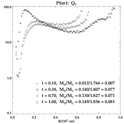
Figure 4: Model PSm1: evolution of the Toomre parameter, $Q_{\rm{T}}$. The disk remains globally stable, as $Q_{\rm{T}}>1$. One local ring (where $Q_{\rm{T}}\approx 1$) develops non-axisymmetry which eventually is damped globally (see Fig. 5).

Table 2 lists the properties of models tested in this study, calculated only from the initially present $M_{0}$. They do not include properties of the subsequent infalling layers, and as such, the bulk values are relevant measures of relative energies and angular momentum, but they are not absolute quantities for the entire collapsar. In addition, we define the dimensionless ratio, $y_{j}$, of the inflow average specific angular momentum, $\bar{j}_{0}=J_{0}/M_{0}$, to the characteristic quantity, $j_{\rm ISCO}$ of the central object (even for the Newtonian potentials, as an approximation), and we discuss further application of this in §11. In order to further explore a wider range of possible LGRB progenitors, various physical properties of the pre-collapse progenitor are rescaled. In particular, we focus on quantities which appear in $Q_{\rm{T}}$, affecting the stability of the forming accretion disk. Scalings of both the shellular and cylindrical rotation profiles are tested, which affect $\Sigma$ by determining the location of centrifugal balance for a fluid element. Similarly, the specific internal energy ($\propto c_{\rm{s}}^{2}$) is decreased, to examine the effects on $\dot{M}$ and the neutrino cooling rates by changing the initial location of a fluid element in the ($\rho,T$) phase space. For comparison, a Newtonian potential is used in two models to gauge the effects of relativity on the collapsar system. Finally, in one model a ‘jet’ is inserted at late times after the formation of a spiral, in order to examine the production of outflows.

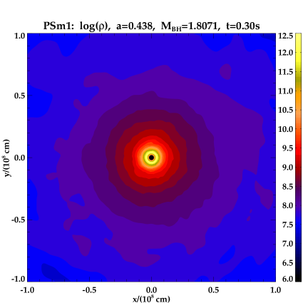
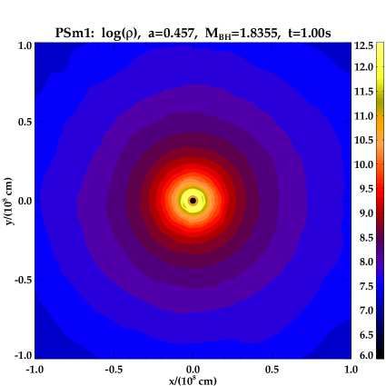
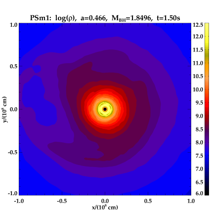
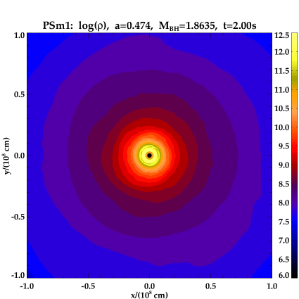
Figure 5: Model PSm1 (equatorial density) closely follows the evolution of $Q_{\rm{T}}$, as the disk is globally stable to hydrodynamic perturbations present in the early phases. A locally unstable region leads to the growth of temporary non-axisymmetric structure, which damps out due to global stability

6 Shellular rotation models

We now describe the evolutions of various models with shellular profiles. In order to appreciate the evolution of a number of the more dynamic models, we also make reference to animations showing the evolution of density ($\rho$), specific entropy per baryon ($s/A$) and entropic function ($K$).

6.1 PSm1

Fig. 4 shows the evolution of $Q_{\rm{T}}$, for the evolving PSm1 accretion disk. Also shown are estimates of the mass of the forming disk compared to central object mass ($\rm{M_{D}/M_{C}}$). As the disk grows, $Q_{\rm{T}}$ approaches the region of instability in one localised region. At late times, the minimum remains just greater than unity throughout the disk, which is therefore predicted to remain globally stable against the development of non-axisymmetric structures (though locally, one region remains near instability). In testing the often-used approximation for classifying stability, it was found that the shape of the $Q^{\prime}_{\rm{T}}$ curve was very similar to that in Fig. 4 but with systematically smaller values, in roughly constant ratio, $Q^{\prime}_{\rm{T}}/Q_{\rm{T}}\approx 70-80\%$. This behaviour remains in the other pseudo-potential systems as well, and only $Q_{\rm{T}}$ has been used in analysis.

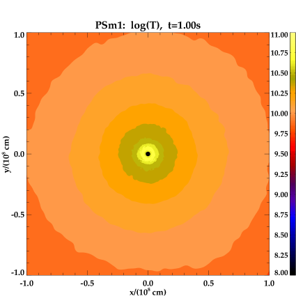
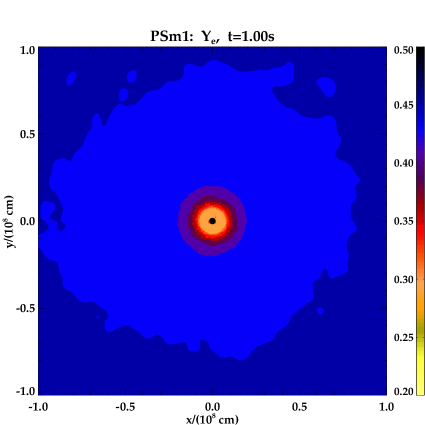
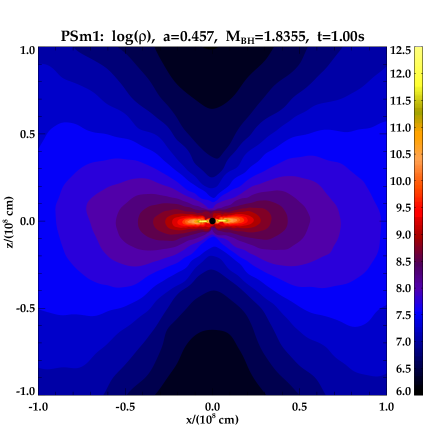
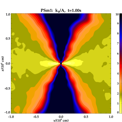
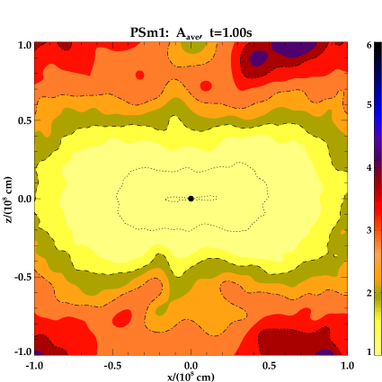
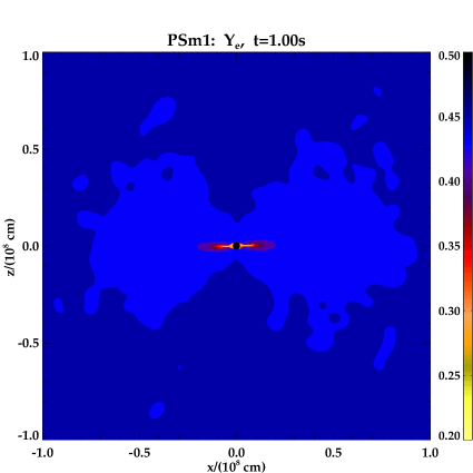
Figure 6: Model PSm1 properties at $t=1.00$ s: $T$ and $Y_{\rm{e}}$ in the equatorial plane (top); in the vertical plane, $\rho$ and $s$ (middle), and $Y_{\rm{e}}$ and $\bar{A}$ (bottom), for which in the latter are included lines of $\bar{A}=1$ (dotted), 2 (dashed), 3 (dot-dashed), 4 (dot-dot-dashed).

The disk behaviour during evolution, as shown by the equatorial density contours in Fig. 5, closely follows the Toomre stability analysis. Large non-axisymmetric perturbations which appear at early times ($t\sim 0.30$ s) have become globally axisymmetric by $t=1.00$ s. The small, $m=2$ mode in density which is beginning to form at $R\lesssim 10^{7}$ cm (at $t=1.00$ s), where $Q_{\rm{T}}\approx 1$ predicted a locally unstable region, develops into a higher order mode by $t=1.50$ s. While outer regions become temporarily disturbed, the disk remains globally stable and returns to a quasi-steady state by $t=2.00$ s. Thus, the instability remains local and does not lead to the formation of large spirals and to enduring, non-axisymmetric modes. The disk is dense ($\rho>10^{8-12}$) and hot ($T>$ a few MeV), with inner regions reaching electron fractions $Y_{\rm{e}}\lesssim 0.3$, as shown in the top panel of Fig. 6.

Figure 7: Radial velocity profile of PSm1 at $t=1.00$ s, for which ‘diamonds’ and ‘+’ show outflows and inflows, respectively.

The vertical disk structure is shown in the lower panels of Fig. 6. The density and specific entropy show the inner ‘thin disk’ region extending out to $R_{\rm{T}}\lesssim 2\times 10^{7}$ cm, with an extended quasi-thin disk out to $\approx 2~{}R_{\rm{T}}$. A large ‘corona’ of hot ($T\sim 1$ MeV) and fairly dense material extending from the equatorial plane is in vertical near-equilibrium (i.e., not in an outward-driven wind, but instead, with relatively small velocities) and balances the continued infall, with uniform $Y_{\rm{e}}$ and dominated by material with $\bar{A}\leq 4$. At irregular intervals, radial outflows are produced in the equatorial plane (Fig. 7, bottom), with velocities up to $\sim 1000~{}\rm{km~{}s}^{-1}$, which carry the low-$\bar{A}$,-$Y_{\rm{e}}$ material outwards.

Figure 8: Model PSm1: evolution of mass accretion rates and neutrino luminosity. After a brief period of rapid accretion of low-$j$ material, $\dot{M}$ decreases rapidly as the disk reaches a steady, axisymmetric state. The neutrino luminosity behaves similarly; after an initial period of rapid cooling of dense, shock-heated material, $L_{\nu}$ decreases below 1 foe s^-1.

The rate of accretion, $\dot{M}$, onto the central object is shown in Fig. 8, along with the disk neutrino luminosity, $L_{\nu}$. During early times, $\dot{M}$ is large (while low angular momentum material accretes quasi-spherically), as is $L_{\nu}$ since infalling material shocks around the PNS surface and begins to cool rapidly, with a maximum just as $\dot{M}$ begins to decline. By late times, a stable disk has formed with steady (predominantly equatorial) accretion, and neutrino production decreases. By Eq. (4), these values of $\dot{M}$ are at least a factor of 3-4 too low to produce $\dot{E}_{\rm{B-Z}}\approx\dot{{\it E}}_{\rm{GRB}}$.

For neutrinos, even utilising a reasonably optimistic annihilation efficiency, $\eta_{\nu\bar{\nu}}L_{\nu}\ll\dot{E}_{\rm{GRB}}$. Therefore, this model will not produce a successful LGRB by either mechanism, as accretion rates from the usual viscous processes by which the thin $\alpha$-disk evolves are too low. The collapsing material possesses too much angular momentum and thermal support to be globally unstable, even with large amounts of neutrinos being produced from the inner regions.

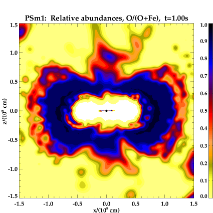
Figure 9: For model PSm1, contours compare the relative locations of O and Fe produced by the disk and inner region in NSE (vertical slice above the equatorial plane). In the central (empty) region, amounts of both elements are negligible.

To analyse the collapsar from the point of view of producing a HN, we have calculated the quantities of various elements produced in the disk and inner regions in NSE, which are given for PSm1 (and for other models) in Table 3. As noted above, light elements dominate the disk material, and most of the heavy metals are produced in the corona and shocked infall regions. For PSm1, the NSE mass of ⁵⁶Ni remains fairly constant at $0.02~{}\textrm{M}_{\odot}$, which is nearly double the mass of ⁵⁴Fe ($0.012~{}\textrm{M}_{\odot}$) and roughly equal to total elemental Fe ($0.021~{}\textrm{M}_{\odot}$, though the iron content slowly increases with time). Therefore, NSE-nucleosynthesis in and around the (steady) collapsar disk falls short of the amount of ⁵⁶Ni required to power the bright HNe by roughly an order of magnitude.

A comparison of the relative production of elemental Fe and O in the fluid elements is shown in Fig. 9. As the disk settles into a steady flow, there seems to be only a slight preference for Fe being produced in the polar direction and O equatorially in the coronae around the dense disk. It should be noted that what is plotted is only the relative, local abundances, and that the total mass of O produced in this case is several orders of magnitude less than the Fe. However, this mass difference may be unsurprising given that Fe, unlike O, is an NSE end product which dominates the mass-fraction for a large area of relevant ($\rho,T$) phase space (cf. Appendix C).

Table 3: Representative NSE-nucleosynthetic yields (in $\textrm{M}_{\odot}$) at late times for each model. The largest fluctuations in elemental abundance ($>$ order of magnitude) occured in PSdsq2, for which the values are given at two times.

Model [$t$ (s)]	56Ni	Co	Fe	54Fe	Cr	Ca	Si	O	4He	$n$	$p$
PSm2 [1.0]	$10^{-4.0}$	$10^{-2.7}$	$10^{-2.0}$	$10^{-2.5}$	$10^{-2.5}$	$10^{-4.4}$	$10^{-4.0}$	$10^{-5.9}$	0.17	0.03	0.02
PSm1 [1.0]	0.02	0.01	0.03	0.12	$10^{-2.2}$	$10^{-3.5}$	$10^{-3.5}$	$10^{-5.4}$	0.38	0.19	0.14
PSdsq2 [1.0]	$10^{-2.2}$	$10^{-2.2}$	0.02	0.01	$10^{-2.7}$	$10^{-3.7}$	$10^{-3.7}$	$10^{-5.5}$	0.25	0.52	0.35
PSdsq2 [1.25]	$10^{-8.3}$	$10^{-5.4}$	$10^{-4.8}$	$10^{-6.0}$	$10^{-5.0}$	$10^{-6.2}$	$10^{-6.4}$	$10^{-6.6}$	0.09	0.15	0.10
PSd2 [0.42]	0.04	0.03	0.07	0.05	$10^{-2.2}$	$10^{-3.0}$	$10^{-3.1}$	$10^{-6.0}$	0.14	0.43	0.25
PCm1 [1.0]	$10^{-2.3}$	0.01	0.04	0.02	$10^{-2.1}$	$10^{-3.7}$	$10^{-3.4}$	$10^{-5.7}$	0.54	0.35	0.31
PCdsq2 [0.58]	0.01	0.02	0.05	0.03	$10^{-2.2}$	$10^{-3.4}$	$10^{-3.3}$	$10^{-5.7}$	0.27	0.50	0.35
PCd2 [0.44]	0.03	0.03	0.06	0.04	$10^{-2.2}$	$10^{-3.1}$	$10^{-3.2}$	$10^{-5.6}$	0.19	0.45	0.26
PSm1Kd5 [1.0]	$10^{-3.0}$	$10^{-2.4}$	0.02	$10^{-2.2}$	$10^{-2.4}$	$10^{-4.1}$	$10^{-3.7}$	$10^{-5.6}$	0.40	0.46	0.36
PSd2Kd5 [0.40]	0.10	0.02	0.03	0.02	$10^{-2.5}$	$10^{-3.2}$	$10^{-3.5}$	$10^{-6.0}$	0.10	0.48	0.24
NSm1 [1.0]	$10^{-4.2}$	$10^{-2.7}$	$10^{-2.1}$	$10^{-2.7}$	$10^{-2.5}$	$10^{-4.7}$	$10^{-4.2}$	$10^{-6.1}$	0.18	0.01	0.07
NSd2 [0.35]	0.03	0.03	0.07	0.05	$10^{-2.1}$	$10^{-3.0}$	$10^{-3.0}$	$10^{-5.6}$	0.16	0.42	0.23
PSdsq2J [1.25]	$10^{-5.1}$	$10^{-7.1}$	$10^{-3.3}$	$10^{-4.0}$	$10^{-3.7}$	$10^{-5.9}$	$10^{-5.5}$	$10^{-6.5}$	0.17	0.16	0.10

We now investigate the three regions of potential non-NSE nucleosynthesis as mentioned in §4.6. For region (i), some equatorial outflow material reached velocities of order $10^{3}~{}\rm{km~{}s}^{-1}$ at $R\sim 10^{8}$ cm, where $Y_{\rm{e}}\approx 0.43-0.45$ (Fig. 6). The entropy through much of the disk is quite low, but in the outermost regions and corona reaches $\sim 10~{}k_{\rm{B}}/A$. However, efficient ⁵⁶Ni-production would probably require significantly greater ejection velocities as well as higher entropy.

There is not a great deal of outflow vertically from the disk for region (ii). The coronal material is optically thin to neutrinos and possesses a quasi-steady vertical structure; the velocities (not shown) of fluid elements are relatively small ($\ll 0.1~{}c$) and non-uniform, except in the azimuthal direction (for near-Keplerian rotation). Therefore, these coronal regions do not appear to be a possible site for $r$-process nucleosynthesis, and these characteristics are similar throughout the disks analysed here.

Finally, for region (iii) near the inner edge of the disk, some material has $Y_{\rm{e}}\approx 0.3$, which is beneficial for $r$-processing, though the specific entropy in these regions is quite low ($s/A\sim 1$) due to efficient neutrino cooling. However, as seen in Fig. 6, high-$s$ regions surround the inner disk edge, where material is still less neutron rich $Y_{\rm{e}}\approx 0.43-0.45$. Furthermore, unlike in region (ii) where vertical motion of material is inhibited by continued infall, after the initial core-collapse the cone around the rotation axis has a relatively low density. One might expect vertical trajectories in this region either from material shock-heated to form a high entropy ‘bubble’ which rises, or from material swept up in the collimated outflow which creates the actual LGRB (discussed briefly in §9).

6.2 PSdsq2

Figure 10: Model PSdsq2: evolution of the Toomre parameter, $Q_{\rm{T}}$. By $t=0.70$ s, a significant fraction of the disk is unstable ($Q_{\rm{T}}<1$), and spiral structure develops dynamically.

We now investigate a model ($v_{\phi}$ globally decreased by a factor of $\sqrt{2}$) with one half of the $E_{\rm{kin},\phi}$ of the marginally unstable PSm1. The evolution of $Q_{\rm{T}}$ is shown in Fig. 10, as well as the disk/central object mass ratios, which are significantly larger than in the previous model. A large part of the inner disk has $\rm{Q_{T}}<1$ and is therefore predicted to be unstable to density perturbations. Indeed, non-axisymmetric structures form by $t=0.50$ s and Fig. 11 (top) shows spirals in the density evolution as well as localised density clumps. The same figure shows the effect of shocks in transferring kinetic energy into thermal, easily seen in the $T$-profiles. The (online) animations of density and specific entropy illustrate the full dynamics of the global behaviour of the disk, in particular the creation of oscillating, $m=0$ flows in the equatorial plane.

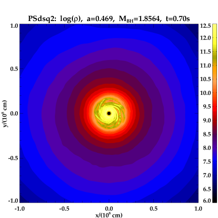
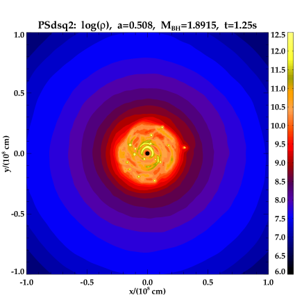
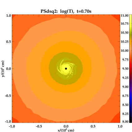
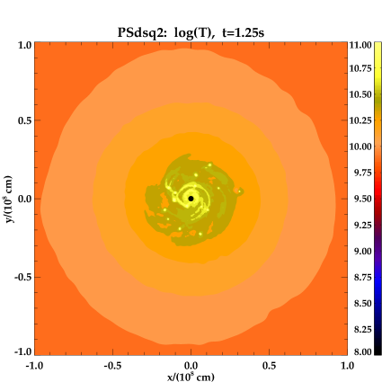
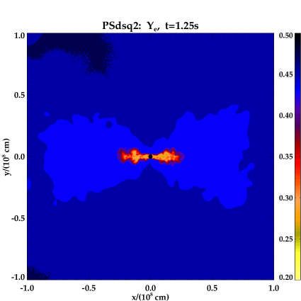
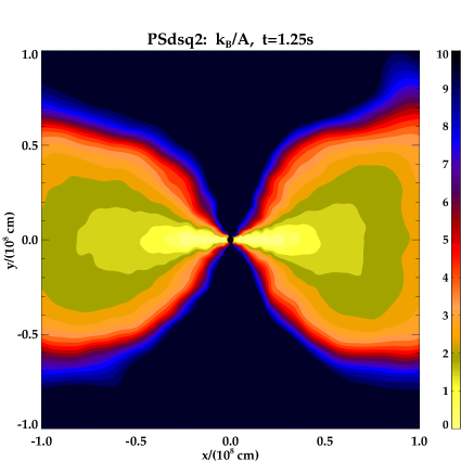
Figure 11: Model PSdsq2 in the equatorial plane, non-axisymmetric evolution of $\rho$ and $T$ at $t=0.7$ s (top) and $t=1.25$ s (middle); spiral structure develops and leads to shocks and angular momentum transfer. (bottom) Electron fraction and specific entropy in the vertical plane at $t=1.25$ s.

The mass accretion and neutrino production rates are shown in Fig. 12, with the same initial phase of low-$j$ accretion. Even after the initial onset of spirals at $t>0.50$ s, $\dot{M}$ remains low until $t>1.10$ s, at which time spikes of rapid accretion develop. In this case accretion rates with $\dot{M}>0.6~{}\textrm{M}_{\odot}~{}\textrm{s}^{-1}$ give rise to $\dot{E}_{\rm{B-Z}}\approx 5~{}\textrm{foe}~{}\textrm{s}^{-1}>\dot{\it{E}}_{\rm{GRB}}$. $L_{\nu}$ increases by an order of magnitude during the rapid accretion to $\approx 30~{}\textrm{foe}~{}\textrm{s}^{-1}$. Therefore, while the system provides conditions for a central engine of sufficient power to create a GRB jet via the B-Z mechanism, the process of neutrino annihilation is probably too inefficient to produce a ‘successful’ jet, as $\dot{E}_{\nu}\approx 0.3~{}\textrm{foe~{}s}^{-1}<\dot{E}_{\rm{GRB}}$.

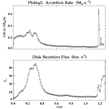
Figure 12: Model PSdsq2: mass accretion rates and neutrino luminosity.

The size of the $T>1$ MeV inner region of this collapsar is larger than that of PSm1, and a much smaller mass of Fe-group elements is present, particularly by $t=1.25$ (Table 3). As a consequence, only a very small amount of ⁵⁶Ni is created, and there is no preferential production of Fe in the polar direction at late times. The region of $\bar{A}<4$ material is less flattened along the equatorial plane, and likewise the distribution of O vs Fe is less polarised (particularly due to the extremely low iron content at late times).

The coronal structure (Fig. 11, bottom panel) is smaller than that in PSm1. It remains fairly steady, even during periods of outflow, and the non-aligned nature of the (non-azimuthal) components of velocity vectors is shown in Fig. 13, ruling out case (ii) outflows for nucleosynthesis. Peak equatorial outflows reach a factor of a few higher than for PSm1, but are still probably too low for case (i). The low-entropy region has a smaller vertical height from the equatorial plane, and material with higher $s/A$ and moderate $Y_{\rm{e}}$ lies quite close to the central object in this model (Fig. 11). Minimum values of the electron fraction in the disk have decreased due to high $T$ and $\rho$ of the shocked regions to roughly $Y_{\rm{e}}=0.25$, but the specific entropy remains low. Again, case (iii) outflows in the presence of a jet flow remain the most likely location for significant ⁵⁶Ni-production.

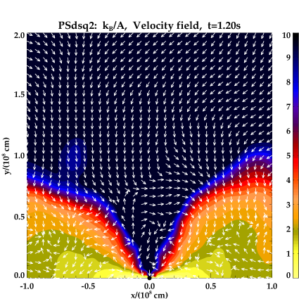
Figure 13: Specific entropy contours with normalised velocity vector field showing direction of flow in vertical slice half-plane (above equatorial plane) during accretion phase. The flow directly above the poles shows small turbulent eddies.

6.3 PSd2

Figure 14: By $t=0.25$ s, part of the disk has reached an unstable state ($Q_{\rm{T}}\approx 1$), and a larger extent of the disk has become unstable by $t=0.30$ s.

The model PSd2 ($v_{\phi}$ decreased by a factor of 2) possesses 25% of the $E_{\rm{kin},\phi}$ of PSm1 and continues the trend of showing greater instability at earlier times after collapse ($t\approx 0.20-0.25$ s). Fig. 14 shows the evolution of $Q_{\rm{T}}$ and the increasing disk/central object mass ratio. Fig. 15 shows the perturbations evolving as a complex configuration: tightly wound spirals develop into filaments within a global $m=2$ mode (full evolution in the online animations). The inner region is comprised of alternating dense ‘fingers’ and shocked flow with higher entropy. Though intially a smaller disk forms than in previous models, the non-axisymmetric structure extends to larger radii.

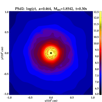
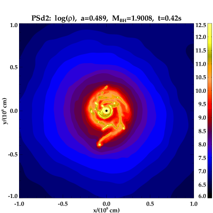
Figure 15: Model PSd2 in the equatorial plane, non-axisymmetric evolution of $\rho$ at $t=0.30,0.42$ s. Small structures develop quickly into global modes and angular momentum transfer.

Figure 16: Model PSd2: mass accretion rates and neutrino luminosity.

For much of the disk evolution, the mass accretion rate is consistently high (Fig. 16). After the influx of low-$j$ material, non-axisymmetric structures form ($t>0.20$ s) and disk accretion increases to $\dot{M}=0.4~{}\textrm{M}_{\odot}~{}\textrm{s}^{-1}$, peaking at the high rate of $\dot{M}\approx 1.2~{}\textrm{M}_{\odot}~{}\textrm{s}^{-1}$. This is reflected also in the neutrino luminosity, which reaches $L_{\nu}\gtrsim 100~{}\textrm{foe}~{}\textrm{s}^{-1}$. Therefore, in this model a successful central engine for a GRB jet is produced by both mechanisms being examined in this study. High accretion rates (with $a\approx 0.5$ and assuming a large, central $B$-field) lead to $\dot{E}_{\rm{B-Z}}\approx\dot{\it{E}}_{\rm{GRB}}$, while the large neutrino production from the shock-heated disk leads to $\dot{E}_{\nu}>\dot{E}_{\rm{GRB}}$ (assuming a reasonable $\nu$-annihilation efficiency).

As in the previous models, mainly light elements constitute the disk. Although the inner regions here produce a much greater amount of heavy elements, $0.048~{}\textrm{M}_{\odot}$ of ⁵⁴Fe, $0.069~{}\textrm{M}_{\odot}$ of Fe, $0.029~{}\textrm{M}_{\odot}$ of Co and $0.037~{}\textrm{M}_{\odot}$ of ⁵⁶Ni, the latter remains below that required to power typical HNe (though, as noted previously, a repetition of accretion events may additively increase abundances). The outflow velocities in the equatorial region reach $5\times 10^{8}<v_{\rm{R}}\lesssim 10^{9}~{}\textrm{cm}~{}\textrm{s}^{-1}$. Much of the material at the outer edge of the disk has high specific entropy with $Y_{\rm{e}}\sim 0.45$, making case (i) outflows a possible site for non-NSE nucleosynthesis. While there is some vertical flow from the equatorial plane, most material remains confined to the coronal regions, limiting the possibility of case (ii) processes.

There is very little asymmetry observed in Fe and O, with production of the latter slightly increased along the equatorial plane near the coronal structures.

6.4 PSd5, PSm2

Neither model PSd5 nor PSm2 ($v_{\phi}$ decreased by a factor of 5 and increased by a factor of 2, respectively) results in a successful LGRB progenitor. In model PSd5, the accretion onto the central object remains quasi-spherical, with 45% of $\dot{M}$ coming from the polar direction even at t = 0.20 s. The infall rate is quite steady, with no outflows. This model has too little rotation to form a significant disk structure or a potential LGRB, and it shows very little polarisation in element abundances.

In PSm2, the Toomre parameter remains $\geq 2$ at all times. Since PSm1, with 25% of the kinetic energy of this model, was only locally unstable, it is unsurprising that this disk appears to be globally stable. The mass of dense ($\rho>10^{8}\textrm{g}~{}\textrm{cm}^{-3}$) disk material is significantly less than that of model PSm1, and by $t=1$ s the central object has accreted approximately half as much mass. In this case, the distribution of elemental O is significantly polarised along the equatorial plane.

Results for both models are given in Tables 3 and 4.

7 Cylindrical rotation models

We briefly discuss the cylindrical rotation profile models, which have lower $E_{\rm{kin},\phi}$ but higher $J_{0}$ than the shellular models. In general, the results for respective scalings of velocity for each series are qualitatively similar.

7.1 PCm1

The evolution of $Q_{\rm{T}}$ and of the system’s disk/central object mass ratios are shown in Fig. 17 for PCm1 (full $v_{\phi}$). In this model the collapsing material forms a disk without any locally unstable region, even though the disk average $Q_{\rm{T}}\gtrsim 10$ is less than in PSm1.

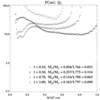
Figure 17: For PCm1, $Q_{\rm{T}}\gg 1$ for the entire evolution, and the disk remains stable.

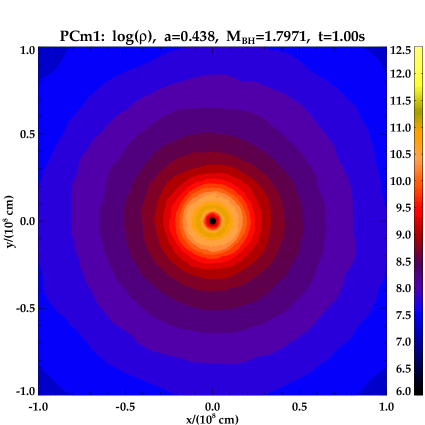
Figure 18: Equatorial density profile for PCm1, which shows peak density less than PSm1.

The densities in the inner disk region remain approximately an order of magnitude less than in PSm1, with a slowly decreasing density profile in the outer regions (Fig. 18). The temperature and radial velocity profiles are similar, although $Y_{\rm{e}}$ remains above 0.35. In general, the vertical structure and the relative locations of Fe and O are similar to those of PSm1. Roughly a factor of five less ⁵⁶Ni is produced in PCm1, which produces $\approx 60\%$ more Fe and ⁵⁴Fe instead (Table 3).

After a brief accretion period of low-$j$ material, $\dot{M}$ settles to $\approx 0.03$ M${}_{\odot}~{}\textrm{s}^{-1}$. Similarly, even with 100% neutrino annihilation efficiency, $\dot{E}_{\nu}$ remains below $\dot{E}_{\rm{GRB}}$. Therefore, this model, like PSm1, does not appear to be a candidate for either a LGRB or a HN.

7.2 PCdsq2

The evolution of $Q_{\rm{T}}$ for PCdsq2 ($v_{\phi}$ decreased by a factor of $\sqrt{2}$) is shown in Fig. 19. The disk becomes unstable by $t=0.35$ s, earlier than for PSdsq2 and with a larger radial extent. The resulting formation of spirals and an $m=2$ structure is shown in Fig. 20. High velocity radial outflows form, $v_{\rm{R}}\sim 10^{9}~{}\textrm{cm~{}s}^{-1}$, carrying material with $Y_{\rm{e}}\approx 0.43$ outward. The values of $\bar{A}$ increase much more rapidly with radius than in PSdsq2, with much of the material in the outflow regions having $\bar{A}>4$.

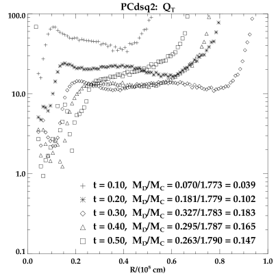
Figure 19: $Q_{\rm{T}}$ evolution for PCdsq2, which is unstable by $t=0.35$ s.

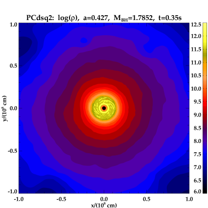
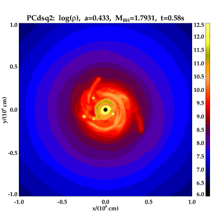
Figure 20: Evolution of density perturbations in PCdsq2.

Figure 21: Model PCdsq2: evolution of mass accretion rates and neutrino luminosity.

In the vertical plane the coronal regions extend to greater height, with a much larger amount of material with $Y_{\rm{e}}\approx 0.43$. Again, the average nucleon number increases and the temperature drops more quickly outside of the main disk/coronal area. The outer corona again contains O preferentially, with the Fe abundance dominating at larger radii. The amount of ⁵⁶Ni ($0.096~{}\textrm{M}_{\odot}$) remains below HN values, however, by a factor of 3-5. This is similar to PSdsq2, where O was more prevalent in all regions, and significantly smaller amounts of Fe-group elements were produced.

After the initial infall of low-$j$ material, accretion rates (shown in Fig. 21) remain low, $\dot{M}<0.05~{}\rm{M}_{\odot}~{}\textrm{s}^{-1}$, even after the formation of spiral structure, although there is an upturn at late times. Neutrino luminosity is fairly high at $L_{\nu}\approx 10~{}\textrm{foe~{}s}^{-1}$, but $\dot{E}_{\nu}$ remains below $\dot{E}_{\rm{GRB}}$ for reasonable annihilation efficiencies.

7.3 PCd2

As in the shellular case, PCd2 ($v_{\phi}$ decreased by a factor of 2) becomes unstable to the formation of non-axisymmetric structure quickly ($t<0.20$ s, Fig. 22). Fig. 23 shows the spiral modes which create shocks in the fluid flow. The evolution of structure, with the development of finer spirals followed by a global $m\approx 2$ mode, is very similar to that of PSd2. Eventually, moderate-$Y_{\rm{e}}$ material moves outward in the equatorial plane due to the transfer of angular momentum in the disk.

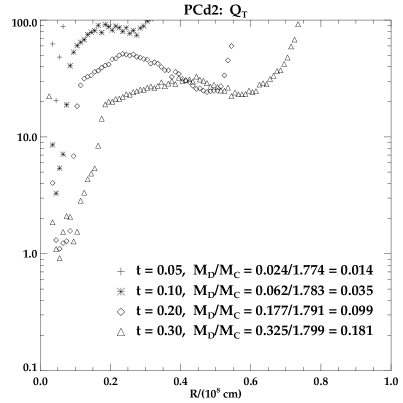
Figure 22: $Q_{\rm{T}}$ evolution for PCd2, which is unstable by $t\gtrsim 0.20$ s.

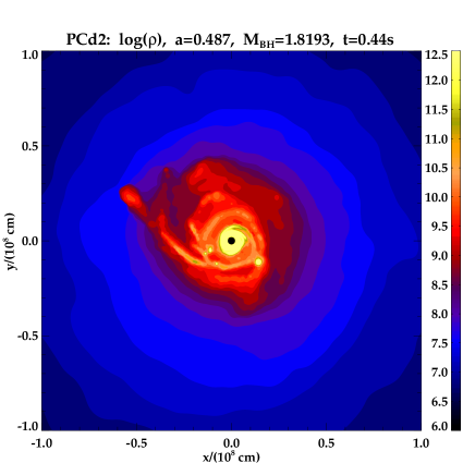
Figure 23: Density structure in the equatorial plane for model PCd2 at $t=0.44$ s.

In the vertical plane again $\rho$, $s/A$ and $Y_{\rm{e}}$ decrease more slowly with distance from the equatorial plane than in the equivalent shellular model, PSd2. ⁵⁶Ni and Fe are produced in very similar quantities to those of PSd2. Typically, the outer corona contains O preferentially, with Fe abundances being greater at larger radii.

During the spiral structure phase, accretion rates begin near $\dot{M}\lesssim 0.1~{}\textrm{M}~{}\textrm{s}^{-1}$, increasing to $\dot{M}\lesssim 0.4~{}\textrm{M}~{}\textrm{s}^{-1}$ at late times. The neutrino luminosity is fairly high during the spiral structure phase and increases to $L_{\nu}=100-150~{}\textrm{foe~{}s}^{-1}$. This model therefore provides sufficient fuel for a LGRB central engine for both the B-Z mechanism and $\nu$-annihilation, as did PSd2.

8 Low temperature models

The low temperature (shellular) models produced results very similar to those with similar rotation profiles discussed above in §6. Comparisons between the relevant models are discussed here.

8.1 PSm1Kd5

The mass of the disk which forms in PSm1Kd5 (full $v_{\phi}$) is greater that of PSm1. The shapes of the $Q_{\rm{T}}$ profiles are similar, with PSm1Kd5 tending to lower values, though its minimum value increases after $t\approx 0.70$ s, and the disk remains globally stable throughout its evolution (Figs. 2425). Much smaller regions of outflow are produced and with lower $v_{\rm{R}}$, due to the greater stability of the disk.

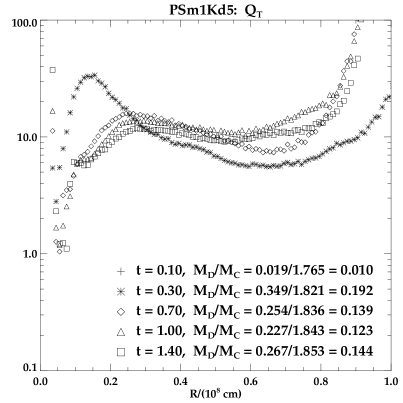
Figure 24: $Q_{\rm{T}}$ evolution for PSm1Kd5, which remains stable globally.

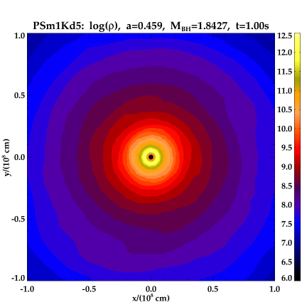
Figure 25: Density in the equatorial plane for PSm1Kd5, which has a very similar profile to that of PSm1, excepting the local instability (cf. Fig. 5).

Through the first $1.00$ s, PSm1 and PSm1Kd5 have similar temperature profiles in the equatorial plane. In the latter, density decreases and specific entropy increases more slowly with radius, and, while the electron fraction is greater in the inner region ($Y_{\rm{e}}\approx 0.30$), $Y_{\rm{e}}$ increases slowly so that a larger region contains material with $Y_{\rm{e}}\approx 0.43-0.45$; $\bar{A}$ behaves similarly.

Vertically, in PSm1Kd5 density decreases rapidly with distance from the equatorial plane, and a smaller corona surrounds the disk than in PSm1. In this region, there is a larger extent of low $s/A\leq 1$ material, before the entropy increases rapidly. The electron fraction behaves similarly in the corona, with $Y_{\rm{e}}$ mainly $\approx 0.43$. The amount of ⁵⁶Ni produced is smaller by an order of magnitude, as are the total masses of the Fe-group elements calculated here in general (Table 3). The relative regional distributions of O and Fe are similar to those of PSm1, with a slightly smaller coronal extent of O.

Both $\dot{M}$ and $L_{\nu}$ closely resemble those for PSm1. After the initial accretion of shock-heated, low-$j$ material, accretion rates settle to $\dot{M}\approx 0.03~{}\textrm{M}_{\odot}~{}\rm{s}^{-1}$, and neutrino luminosity goes to $L_{\nu}\approx 0.1\textrm{~{}foe~{}s}^{-1}$. Therefore, model PSm1Kd5 is also unable to produce a successful LGRB.

8.2 PSd2Kd5

The shapes of the $Q_{\rm{T}}$ curves for PSd2Kd5 ($v_{\phi}$ decreased by a factor of 2) shown in Fig. 26 are very similar to those of PSd2, with the former having $\approx 10\%$ lower values. For $t<0.20$ s, the disk masses are nearly identical as well. Again, tightly wound spirals develop into ‘finger-like’ substructure in a global $m=2$ mode (Fig. 27). It is perhaps surprising that the thermal and specific entropy structures are also nearly identical to those of PSd2, despite an initially large difference in internal energy. Also, the $\bar{A}$ and $Y_{\rm{e}}$ values are very similar for both models. However, the outflow velocities in the equatorial plane are much greater in PSd2Kd5, reaching $v_{\rm{R}}>0.1c$.

Figure 26: For PSd2Kd5, $Q_{\rm{T}}$ becomes unstable after $t=0.20$ s, slightly earlier than PSd2; the shapes of the curves are very similar, with PSd2Kd5 being $\approx 10\%$ less (cf. Fig. 14).

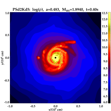
Figure 27: Equatorial density profile for PSd2Kd5, which shows very similar late time structure to PSd2 (cf. Fig. 15).

The vertical profiles of PSd2Kd5 closely resemble those of PSd2, but the coronal regions are smaller in the former, and $\rho$ decreases more rapidly with distance from the equatorial plane. The relative locations of Fe and O production follow those in PSd2. However, the amounts of Fe-group elements produced are quite different (Table 3). Here, $0.10~{}\textrm{M}_{\odot}$ of ⁵⁶Ni is made, approximately three times the amount in PSd2 and only a factor of a few below that which is estimated for some HNe. The masses of the competing end-products, $0.017~{}\textrm{M}_{\odot}$ of ⁵⁴Fe and $0.029~{}\textrm{M}_{\odot}$ of Fe, are a factor of three lower than in PSd2.

In this model accretion reaches very high rates, $\dot{M}\approx 1~{}\textrm{M}_{\odot}~{}\textrm{s}^{-1}$ at peak, with an average of $\dot{M}\approx 0.25-0.30~{}\textrm{M}_{\odot}~{}\textrm{s}^{-1}$ otherwise (Fig. 28). The neutrino flux reaches the high values of $L_{\nu}>200~{}\textrm{foe~{}s}^{-1}$, although it remains below $50~{}\textrm{foe~{}s}^{-1}$ for much of the evolution. Therefore, while at peak values both $\dot{E}_{\rm{B-Z}}$ and $\dot{E}_{\nu}$ are $>\dot{E}_{\rm{GRB}}$, the B-Z mechanism appears to be significantly better for providing a longer duration central engine.

Figure 28: Model PSd2Kd5: evolution of mass accretion rates and neutrino luminosity.

9 Simple jet test, PSdsq2J

In order to test the behaviour of the collapsar flow in the presence of a collimated outflow, we implemented a very simple ‘jet’ structure originating from the central object (starting with model PSdsq2). This was not intended to be a physically realistic jet, but merely a toy model to gain insight into affected regions of the system, i.e. in disk structure, in the nature of any coronal material swept outward, etc.

The prescription inserted into PSdsq2 at $t=1.10$ s was that a narrow jet region with polar angular radius of $\theta=10^{\circ}$ around the rotation axis developed and grew quickly. An acceleration directed along the envelope of the jet, away from the equatorial plane, was applied to every fluid element which approached this region to within a small fraction of its smoothing length.

In Fig. 29, model PSdsq2J is shown 0.10 s after the insertion of the jet. A comparison with the same model without a jet in Fig. 13 shows that the vertical structures are affected only slightly, but most importantly, high $s/A$ material (with moderate $Y_{\rm{e}}$) is carried upwards from the corona and inner edges of the disk at high velocities, $0.05$-$0.1c$. These conditions make the inner disk region a strong candidate for producing large amounts of ⁵⁶Ni in outflows. We note, too, that the vertical outflow material becomes more likely to form Fe-group elements, assuming NSE is maintained; therefore, the polar direction becomes more Fe-rich, while the equatorial plane remains O-rich, as in polarised HNe. Explosive nucleosynthesis in the jet itself may also be a source of heavy elements such as ⁵⁶Ni, though the abundances which can be produced remain uncertain (e.g., Nagataki, Mizuta & Sato, 2006).

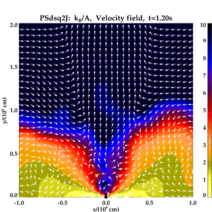
Figure 29: Specific entropy contours with normalised velocity vector field showing direction of flow in vertical slice half-plane (above equatorial plane) for comparison with Fig. 13. Material in coronal regions retains small, turbulent velocities. A strong vertical outflow is created by the jet.

10 Comparing GR and Newtonian potentials

A simple test to gauge the effects of including GR was made by utilising a purely Newtonian central potential in (shellular) simulations with full rotation (model NSm1) and with $v_{\phi}$ decreased by a factor of 2 (model NSd2). In general, the results are quite similar to those using the SEP pseudo-potential (PSm1 and PSd2, respectively).

Fig. 30 shows $Q_{\rm{T}}$ for NSm1. The greatest difference occurs in the minimum-region which nears instability, which is $\approx 50\%$ wider in the pseudo-potential system. The result is that the NSm1 disk remains both globally and locally stable, without the formation of non-axisymmetric structures which developed in the PSm1 model. Due to this (temporary) lack of perturbation, the radial outflow is much lower in the Newtonian case.

The profiles of hydrodynamic and microphysical quantities, in both equatorial and polar directions, are very similar. However, NSm1 produces orders of magnitude less ⁵⁶Ni and a factor of five less Fe than PSm1. The $\dot{M}$ and $L_{\nu}$ values are typically $\approx 15-20\%$ greater in NSm1.

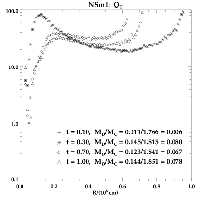
Figure 30: Evolution of $Q_{\rm{T}}$ for the Newtonian, shellular model, NSm1.

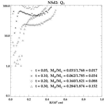
Figure 31: Evolution of $Q_{\rm{T}}$ for the Newtonian, shellular model with reduced rotation, NSd2.

For the reduced velocity case, the $Q_{\rm{T}}$ curves for NSd2 (Fig. 31) closely resemble those of its pseudo-potential analogue, PSd2. Moreover, the structural, hydrodynamic and nuclear constituent properties of the evolving disk appear similar, as well. In this case, the only difference in Fe-group production appears in ⁵⁶Ni, which is $25\%$ less than the amount produced by PSd2. Again, the $\dot{M}$ and $L_{\nu}$ curves for NSm1 are qualitatively similar to those of PSm1 but with the values of each of the former being $\approx 20\%$ greater.

11 Discussion and conclusions

Table 4: Results for the various collapsar models, in terms of maximum accretion rates and energy production. The values of $\dot{E}_{\rm{B-Z,max}}$ have been calculated using Eq. (4). In general, scenarios of $\dot{M}_{\rm{max}}>0.1~{}\textrm{M}_{\odot}~{}\textrm{s}^{-1}$ and $L_{\nu,\rm{max}}>100~{}\textrm{foe}~{}\textrm{s}^{-1}$ produce successful LGRBs (although the profiles for each exhibit rapid fluctuations).

Model	Vel.	$v_{\phi}$	$E_{\rm{th}}$	$y_{j}$	$\dot{M}_{\rm{max}}$	$\dot{E}_{\rm{B-Z,max}}$	$L_{\nu,\rm{max}}$	$M(^{56}\rm{Ni})^{{\dagger}}$	Instability
	Profile	scale	scale	($\bar{j}_{0}/j_{\rm ISCO}$)	(M⊙ s-1)	(foe s-1)	(foe s-1)	(M⊙)	(description)
PSm2	shell	$\times$2	full	65.5	0.023	0.13	0.073	$10^{-4}$	none
PCm1	cyl.	full	full	36.3	0.035	0.20	0.23	0.005	none
PSm1	shell	full	full	32.8	0.032	0.21	0.41	0.020	local perturbation (temp.)
PSm1Kd5	shell	full	/5	32.8	0.027	0.17	0.12	0.001	none (slight non-axis.)
NSm1	shell	full	full	32.8	0.035	0.241	0.20	$10^{-4.2}$	none
PCdsq2	cyl.	/$\sqrt{2}$	full	25.7	0.067	0.38	17.5	0.010	global spirals, late $m=2$
PSdsq2	shell	/$\sqrt{2}$	full	23.1	0.67	8.33	29.7	$10^{-8.3}$	global spirals, late $m=0$
PCd2	cyl.	/2	full	18.2	0.37	2.51	167	0.032	global spirals and $m=1,2$
PSd2	shell	/2	full	16.4	1.23	8.82	121	0.038	global spirals and $m=2$
PSd2Kd5	shell	/2	/5	16.4	1.00	6.49	214	0.101	global spirals and $m=2$
NSd2	shell	/2	full	16.4	0.63	4.41	121	0.029	global spirals and $m=2$
PSd5	shell	/5	full	6.5	-	-	-	-	none (no disk)

${}^{{\dagger}}\,$Estimated at late times in the evolution.

11.1 Numerical timesteps

It was noted in §6.2 that the timesteps in the more dynamic simulations became too short to continue. In Gadget-2 standard hydrodynamical criteria assign the length of time between ‘kicks’ for each SPH particle: the Courant-Friedrich-Levy (CFL) condition, which requires small timesteps for dense material ($\Delta t_{\rm{step}}\propto\rho^{-1}$); and a dynamic condition, which requires small timesteps for particles with rapidly changing velocity ($\Delta t_{\rm{step}}\propto|\textbf{a}|^{-1/2})$.

In the case of collapsars, densities often reach high values, much greater than neutron drip. Similarly, dense matter in the inner disk is shocked by spiral arms, and infalling matter is shocked to high $T$ at the edge of the corona. Finally, particles are removed from the simulation when they are accreted, and during periods of rapid accretion, the computer must keep searching for and recalculating neighbours for nearby un-accreted particles; the material close to the accretion boundary is also typically the densest, meaning that when small amounts accrete, neighbour lists must be recalculated for many particles. For some simulations in this study, the conjunction of these conditions caused timesteps to become quite small, and the computational expense per timestep, quite large.

In order to prevent some of these difficulties, particularly due to neighbour searches when accreting, one may utilise a method of replacing many SPH particles in a high-density region with a single particle, as in Bate, Bonnell & Price (1995). A simplified version of this procedure was tested in some models with only limited success. To avoid these difficulties in future work, more refined numerical treatments of this process and of the accretion will be required.

11.2 Hydrodynamic Instability

In all of the models, the global stability of the collapsar disks consistently depended on the scaling of azimuthal velocity in the progenitor. The dimensionless parameter, $y_{j}=\bar{j}_{0}/j_{\rm ISCO}$, was introduced to characterise the progenitor in terms of relevant quantities; here, systems with values of, very roughly, $10-15<y_{j}\lesssim 30-32$ (with the upperbound seen more directly) were hydrodynamically unstable; for large $y_{j}$, angular momentum stabilises the disk, and for small values, no significant disk forms. The initial velocity profile shape and even the scaling of $E_{\rm{th}}$ by half an order of magnitude had comparatively very little influence. Results from the simulations are summarised in Table 4 (for reference, the scalings of the various model progenitors are included as well). We note that in future studies, the quantity $y_{j}$ may be particularly useful in predicting the behaviour of a collapsar-candidate progenitor.

The full rotation (and $v_{\phi}\times 2$) models proved to be globally stable against forming non-axisymmetric structures, with PSm1 temporarily developing a locally unstable ring. By scaling $v_{\phi}$ in the progenitor by $1/\sqrt{2}$, the resulting disk became unstable to thin spirals which became tightly wound and shocked surrounding fluid. These spirals eventually led to the development of larger, radial oscillations ($m=0$ modes) for PSdsq2 and to global non-axisymmetric structure for PCdsq2. In all cases, scaling $v_{\phi}$ by 1/2 led to the rapid formation of tightly wound spirals and also to the appearance of global $m=1~{}$or$~{}2$ modes which dominated the subsequent disk evolution.

As a general trend, instability set in a number of dynamical timesteps earlier for lower $E_{\rm{kin},\phi}$, with cylindrical models (prefixed with ‘PC’) tending to become unstable slightly more quickly than the shellular ones. The spirals typically formed in the disk within the radial interval of $4-8\times 10^{6}$ cm (of order $20\times GM/c^{2}$), with lower rotation models becoming unstable at the smaller end of the range. We note that for several models, disks formed localised density clumps as well, with signficant repercussions for the accretion rate profile and energetics.

We note that it is not surprising that the $v_{\phi}$ profile of each of the models which formed global structures and non-axisymmetric modes had been scaled downward from that of the original progenitor. The total angular momentum of a binary remnant depends heavily on the redistribution mechanism of the merger process, which remains an area of active research. For the basic progenitor used in this study, the merger prescription had maximised the possible $J$ retained by a remnant, one of three pictures presented by Fryer & Heger (2005). Therefore, it should not be worrying for the general consistency of binary mergers as collapsar progenitors that only the models with scaled-down $E_{\rm{kin},\phi}$ produced globally unstable disks.

Figure 32: A relative comparison of specific angular momentum profiles for the shellular models PSm1, PSdsq2 and PSd2 at $t=1.00,1.25,0.42$ s, respectively. Analogous behaviour occured in the cylindrical and thermally-scaled models. All values are scaled in arbitrary units to the Newtonian, Keplerian profile (line).

11.3 Accretion rates, $\nu$ luminosity

Accretion rates were nearly constant (after accreting low-$j$ material) for the full-rotation models which did not form spirals, settling to be $\approx 0.03~{}\textrm{M}_{\odot}~{}\rm{s}^{-1}$, even in the model with local instability. As shown in Table 4, these rates are too low by a factor of 5-8 to produce a burst via the B-Z mechanism, and the accompanying $\dot{E}_{\nu}$ is also several orders of magnitude below the LGRB limit. Moreover, these models would provide no central engine mechanism for the large variations in observed lightcurves which occur on the order of ms timescales (though other phases of evolution may contribute).

In the $v_{\phi}/\sqrt{2}$ models, accretion rates only increased slightly after the initial onset of the spiral phase and before the formation of global modes; in the PSdsq2 model, the accretion rate then briefly peaked at $\dot{M}>0.65~{}\textrm{M}_{\odot}~{}\rm{s}^{-1}$. The neutrino luminosity was $\approx 10~{}\textrm{foe~{}s}^{-1}$ during the early spiral phase, increasing by a factor of two in PCdsq2 and by a factor of three in PSdsq2 as global modes appeared. While some of the accretion rates reach LGRB energetic requirements, the $\dot{E}_{\nu}$ typically remained too low with the annihilation efficiency taken into account. Model PSdsq2J showed no significant change in disk structure due to the inclusion of a polar jet.

In the $v_{\phi}/2$ models accretion rates were consistently $>0.30~{}\textrm{M}_{\odot}~{}\textrm{s}^{-1}$ and $L_{\nu}>100-150~{}\textrm{foe~{}s}^{-1}$ during the spiral phase, with peak magnitudes occuring in the presence of global modes. Both shellular models (full and reduced $E_{\rm{th}}$) had a higher average accretion rate than the cylindrical model, which averaged and peaked at $\dot{M}\approx 0.1$ and $0.4~{}\textrm{M}_{\odot}~{}\textrm{s}^{-1}$, respectively. These models all produced accretion rates and neutrino luminosities high enough to fuel LGRBs.

In cases with rapid accretion, variations of up to half an order of magnitude in $\dot{M}$ and $L_{\nu}$ occured as rapidly as the snapshot interval of 0.02 s. Such fluctuations have been observed in the spectra of LGRBs, although several factors in the system may combine to produce these, such as jet structure, environment, etc. Here, the bursts of accretion are due in large part to the presence of dense clumps which have been created by the spirals and fragmentation.

We also note that while $\dot{M}$ and $L_{\nu}$ show strong (positive) correlation, no direct scaling appeared between the quantities. In general, the rates of the former appear to make the B-Z mechanism a significantly more likely scenario than $\nu$-annihilation for producing LGRBs, keeping in mind the simplifying assumptions made in calculating both. The neutrino rate was probably too low much of the time, as $L_{\nu}$ only reached above 100 foe$\textrm{~{}s}^{-1}$ at brief intervals for accretion rates typically of $>0.5~{}\textrm{M}_{\odot}~{}\textrm{s}^{-1}$.

The effects of general relativity in the system were non-negligible. During the evolution of the Newtonian models, typical (though not peak) accretion rates and neutrino fluxes were roughly $15-20\%$ higher than in the pseudo-potential models. At the intermediate central object spin rates present in these collapsar simulations ($a\approx 0.5$), the overall difference in potential wells was quite small ($\approx 1\%$, see caption in Table 2). The deviations in disk temperature and structure appear to be the determining factor in the energetics. This stresses the importance of including GR in as realistic a manner as possible in simulations, and further work on this task is being done.

11.4 Nucleosynthesis

In studying NSE-produced materials in the collapsar, it was found that light elements dominated the disk, and that, during the early evolution, the masses of ⁵⁶Ni produced in the corona and beyond were too small to power a HN. Typically the amount of ⁵⁶Ni present in the system remained constant after the early phases of the disk ($t\gtrsim 0.30$ s), when the corona had reached an approximate state of equilibrium. More ⁵⁶Ni was produced in the lower $v_{\phi}$ models, with the greatest amount in the low-$T$ model, $0.10~{}\textrm{M}_{\odot}$. In investigating areas for further production of radioactive Ni, the $v_{\phi}/2$ models produced the strongest equatorial outflows, even though those disks were the smallest; PSd2Kd5 produced the highest outward velocity.

It was also found that, by the inclusion of a simple collimated jet, rapid polar outflows were produced (here, with $v\sim 0.1c$, but this may be strongly model-dependent), which carried high entropy material with moderate and low electron fraction outward. This material from above the disk and the coronal edges which was swept outward may be suitable for forming ⁵⁶Ni, and in some cases, for the $r$-process to manufacture other heavy (neutron-rich) metals. Due to the necessarily high velocity of any outflow, one might expect that, once begun, a relatively large amount of ⁵⁶Ni and Fe-group metals could be deposited outside the disk in a short period of time.

Studying the relative locations of Fe and O did not provide overwhelming evidence for or against the presence of polarised asymmetry, as has been observed and predicted in HNe. In general, O is prevalent in the outer corona, and Fe, outside that region. However, in the presence of the jet, material from the corona would be carried up along the polar axis, with a strong likelihood of heavy elements being manufactured.

11.5 Collapsar implications

While not spanning the lifetime of a typical LGRB, all models in this study ran for a large number of dynamical timescales, and they provide a basis for postulating continued behaviour for long-duration phenomena. It is worth considering the likely behaviour of our models continuing after the end of our simulations, particularly in connection with its implications for both LGRBs and HNe.

Regarding the former, the long-term stability and behaviour of the collapsar disk must be considered. In the scaled $v_{\phi}/2$ models, high accretion rates occured, and the size of the spiral structures grew globally; in the $v_{\phi}/\sqrt{2}$ models, the densest material ($\rho>\rho_{\rm drip}$) tended to be accreted, most likely requiring reformation of the disk to permit high accretion rates. In all of these systems, however, the $Q_{\rm{T}}$ values generally remained low at late times, and a high degree of non-axisymmetric structure remained even in the catastrophic cases, along with dense clumps of material. Moreover, the flattening of specific angular momentum profiles (shown for shellular profiles in Fig. 32) for models with decreased $v_{\phi}$ also suggests continued instability for the disks. With sustained infall, the longterm disk behaviour can then be broadly classified into two possible scenarios: alternating destruction and reformation, and a continual presence with more ‘balanced’ mass loss/gain. Again, these may be evidenced in and also explain some of the variety of observed LGRB lightcurves. While short term fluctuations would be due to clumps and local density differences in the flow, longer term ones may arise from the oscillating behaviour of the disk as a whole.

The details of this behavior may strongly affect HNe as well, in considering the effects of time-integration on heavy element production. The yields from the models in this study must be considered as minima, as the inclusion of non-NSE nucleosynthetic processes will certainly lead to increased amounts of both ⁵⁶Ni, which powers any HN lightcurve, and other Fe-group products, which characterize the non-spherical geometry of the event. In the presence of near-jet outflows, even NSE yields may be enhanced as heavy metals are produced and ejected. Disk evolution, whether proceeding by destruction and reformation or by balanced mass gain and loss, will influence whether metal production is quasi-continual or -discrete, or whether potential Fe-group material is accreted rapidly, delaying any possible HN event.

Within the scope of these trends, there is also, importantly, a wide range of properties obtained from this related sample of LGRB candidates. For example, very different structures of the $\dot{M}$ and $L_{\nu}$ curves were obtained; equatorial outflows of various velocity ranges were produced; the amount of heavy metals (particularly ⁵⁶Ni and Fe), synthesised in the disk and corona varied by orders of magnitude, even for models of similar total angular momentum. Such diversity exists within the observed LGRB/HN population. For example, a system with high accretion rates, low ⁵⁶Ni content in the corona and small outflows in the equatorial plane might produce a bright LGRB with a weak SN explosion (due to low radioactive Ni content). Conversely, a system with low accretion rates and a large mass of ⁵⁶Ni may result in a strong HN with a weak LGRB or with a lower energy XRF, or possibly only a bright, polarised SN. We conclude that dynamically unstable collapsar disks provide a unified and simple explanation for the large variety of these events.

Among the family of potential collapsar progenitors investigated here, the principal discriminating factor appeared to be the overall amount of rotation initially present. Simulation results led to the classification of LGRB candidates by a simple $y_{j}=\bar{j}_{0}/j_{\rm ISCO}$ parametrisation with a window of values for systems that evolved hydrodynamically unstable disks able to fuel a central engine. Importantly, this $y_{j}$ prescription is quite general. Given the diversity of observed LGRBs, the heterogeneity of the GRB-SN/HN connection and the probable relations with phenomena such as XRFs, it is likely that a variety of progenitor scenarios will require examination, including both binary and single-star systems, to fully understand LGRBs. Further considerations may refine progenitor characterisation, but we expect the trends of this study to be broadly applicable across a wide range of possible collapsars.

Additional work should be done to further these results, in particular by including non-NSE nucleosynthetic processes and a more realistic equation of state as well as a physically-motivated jet. These physical inputs are necessary for understanding not only LGRBs themselves but also their particular connection with HNe. Finally, while known to be essential for driving burst jets, magnetic fields were not directly included in this study, and their full role during collapse and disk evolution must be investigated further.

Appendix A Dissipation of MRI, B-field conditions

In consideration of the onset of MRI in an accretion disk, Balbus & Hawley (1991) estimated conditions for non-ideal MHD effects to damp the growth of magnetic modes from dimensional analysis. Specifically, the local dynamical timescale was compared to the diffusion timescale of modes due to finite resistivity and thermal conductivity. This resulted in the following criterion for damping to be negligible (for a $z$-component):

$$\frac{3~{}\Omega_{\rm{K}}\,\chi}{{\it v}^{2}_{\rm{Az}}}\ll 1,$$ (12)

where $\Omega_{\rm{K}}$ is the orbital frequency assuming Keplerian rotation; $v_{\rm{Az}}$, the poloidal Alfvén velocity; and $\chi$, a general diffusion coefficient. They stated that the minimum $B$-field strength for damping to be ignored, and therefore for the MRI to grow nonlinearly, was extremely small for most accretion disks; as a result, a magnetic field, internal or external, of any size would lead to the development of global modes in the disk on dynamical timescales. We investigate the same criteria in the realm of the collapsar disk structure, which has already been noted to be of an extreme nature.

In considering finite electrical resistivity, plasma theory leads to an expression (Spitzer, 1965) for the coefficient in Eq. (12):

$$\chi_{\rm{er}} = \frac{3.8\times 10^{12}\,{\it Z}\,\ln(\Lambda)}{\gamma_{\rm{E}}\,T^{\rm{3/2}}}~{}~{}~{}\rm{cm}^{2}~{}\rm{s}^{-1}~{},$$ (13)

$$\Lambda = \frac{3}{2}\frac{(k_{\rm{B}}{\it T})^{\rm{3/2}}}{{\it Z}\,e^{3}(\pi n_{\rm{e}})^{1/2}}=\frac{4.31\times 10^{20}~{}{\it T}^{3/2}}{(Y_{\rm{e}}\rho)^{1/2}}~{},$$

where $Z$ is ionic charge; $\gamma_{\rm{E}}\approx 1$, the ratio of conductivity to that of an ideal Lorentz gas; and $\ln(\Lambda)$, the Coulomb logarithm. Substituting this coefficient into Eq. (12) for a $Z=1$ (fully ionised) gas, the general condition on the local poloidal $B$-field magnitude for dissipation due to electrical resistivity not to damp out the MRI is:

$$B_{\rm{z,er}}^{2}~{}\gg~{}\frac{2.83\times 10^{27}\ln(\Lambda)~{}\rho}{(RT)^{3/2}}\left(\frac{M}{\textrm{M}_{\odot}}\right)^{1/2}~{}~{}~{}\rm{G^{2}},$$ (14)

where $M$ is the mass of the central BH.

The analogous diffusion coefficient representing the thermal conductivity of the plasma is (Balbus & Hawley, 1991):

$$\chi_{\rm{tc}}=\frac{1.84\times 10^{-5}}{\ln(\Lambda)}T^{5/2}~{}~{}~{}~{}\textrm{cm}~{}\textrm{s}^{-1},$$ (15)

and the corresponding condition on the $B$-field is

$$B_{\rm{z},tc}^{2}\gg\frac{57.8~{}T^{5/2}}{\ln(\Lambda)~{}R^{3/2}}\left(\frac{M}{\textrm{M}_{\odot}}\right)^{1/2}~{}~{}~{}\rm{G^{2}}.$$ (16)

As an example, we check the requirements on the magnetic field in the near-inner regions of the collapsar disk, inserting reasonable values of physical quantities ($R=10^{7}~{}\rm{cm}$, $\rho=10^{11}~{}\textrm{g}~{}\textrm{cm}^{-3}$, $Y_{\rm{e}}=0.4$, $T=10^{10}~{}\rm{K}$, $M/\textrm{M}_{\odot}=3$). The conditions with electrical resistivity and thermal conductivity require that $B_{\rm{z}}\gg 3.3\times 10^{7}~{}\rm{G}$ and $B_{\rm{z}}\gg 2.2\times 10^{7}~{}\rm{G}$, respectively, in order that dissipation is unable to damp out MRI growth. Therefore, the minimal necessary magnetic field strength for nonlinear growth ($B\sim 10^{9}$ G), while not unphysically high, is certainly not negligible, as it is generally for lower density disks.

Appendix B Relativistic pseudo-potentials

The generic task of a pseudo-Newtonian potential is to capture important relativistic aspects without the computational demands of full GR. The most well-known example of such an approximation for a rotation-dominated flow is the Paczyński-Wiita potential for a non-rotating BH, $\Phi_{\rm{PW}}(R)=-M(R-2r_{\rm{g}})^{-1}$ (Paczyński & Wiita, 1980), and there are also similar potentials for motion in the Kerr metric. The accuracy of such potentials can be tested by the comparison of output to exact GR solutions, such as for the location of the innermost stable circular orbit ($R_{\rm{ISCO}}$); the Keplerian orbital velocity ($\Omega_{\rm{K}}$) and the epicyclic frequency ($\kappa$), which are no longer equal, as they are in the Newtonian regime; and the structural and temporal properties of evolving accretion disks, such as specific energy and dissipation.

We note that this involves identifying the Newtonian $R$ in all of these terms with the Boyer-Lindquist (B-L) coordinate, $R_{\rm{B-L}}$. To quantify the resulting deviation involved in this, we compare the proper circumference at $R_{\rm{B-L}}=r_{\rm{in}}$ to the corresponding ‘Newtonian’ value, $2\pi r_{\rm{in}}$, in the equatorial plane. Examples of ($a$, $C_{\rm{B-L}}/C_{\rm{N}}$) are (0,1), (0.5,1.01) and (0.9,1.13). The ratio quickly and monotonically approaches 1 with increasing radius, e.g. for $a=0.9$, it deviates by only 1% at $R=3r_{\rm{in}}$.

For the cases considered here (corotating orbits and not extremely fast BH spin, $0.4\leq a\leq 0.9$), most pseudo-potentials are essentially Newtonian for radii $\geq 20-25~{}r_{\rm{g}}\sim 3-4\times 10^{6}~{}$cm, while also reproducing the correct locations of $R_{\rm{ISCO}}$, which is used as the BH accretion boundary here. However, no single potential is able to reproduce all of the above-noted properties simultaneously to errors within even 20% in the relativistic regimes, and therefore one must choose to focus on certain properties over others depending on the system.

We have considered four different pseudo-potentials for corotating motion around BHs, which we implement as acceleration terms. The $\rm{a_{SEP}}$ acceleration which is implemented in this study was derived by Mukhopadhyay & Misra (2003), and is given in Eq. (6) above. As shown here, this form reproduced most exact GR properties within tolerable limits.

From Artemova, Björnsson & Novikov (1996), the accelerations $F_{5}$ and $F_{6}$ (their Eqs. (13)-(18)) are practically identical, and so we implemented only the former:

$$\rm{a_{Art5}}(\textit{R}) = \frac{M}{\textit{R}^{2-\beta}(\textit{R}-\textit{r}_{1})^{\beta}}\,,$$ (17)

$$r_{1} = 1+\sqrt{1-a^{2}}\,,$$

$$\beta = \frac{r_{\rm{in}}}{r_{1}}-1\,,$$

where $r_{1}$ denotes the location of the event horizon (with radius and spin in units of $M$). Figs. 4-6 of Artemova et al. (1996) show the use of this term in reasonably approximating an optically thick $\alpha$-disk with a low accretion rate by comparing optical depth ($\propto$ surface density) and temperature to a fully relativistic case for different spins. However, a comparison of angular and particularly epicyclic frequencies in Fig. 33 and Fig. 34, respectively, shows great disparities with the exact GR results for $a=0.5$, and these increase with $a$.

Figure 33: A comparison of orbital velocities for different pseudo-Newtonian accelerations, including the exact GR value, for $a$=0.5. ($R$ is measured in units of $M$.)

Figure 34: A comparison of elliptical frequencies for different pseudo-Newtonian accelerations, including the exact GR value, for $a$=0.5. Note: $\rm{a_{Art5}}$ and $\rm{a_{MKep}}$ produce nearly the same frequencies for this BH spin.

Figure 35: A comparison of pseudo-Newtonian accelerations, for $a$=0.5. In these inner regions, $\rm{a_{Art5}}$ and $\rm{a_{MKep}}$ have noticeably larger accelerations than the other potentials, of a factor 2-3 at $R_{\rm{ISCO}}$.

Similar results are produced with the acceleration given by Mukhopadhyay (2002), derived from exact GR solutions for specific energy and angular momentum. His Eq. 12,

$$\rm{a_{MKep}}(\textit{R})=\frac{\textit{M}(\textit{R}^{2}-2\textit{a}\sqrt{\textit{R}}+\textit{a}^{2})^{2}}{\textit{R}^{3}(\textit{R}^{3/2}-2\sqrt{\textit{R}}+\textit{a}^{2})^{2}}\,,$$ (18)

reproduces GR energy dissipation rates calculated very well (his Fig. 1), but does not reproduce well the rotational kinematics, as seen again in Figs. 33-34.

In order to obtain more accurate epicyclic frequencies, Mukhopadhyay & Misra (2003) integrated a function approximating the GR value of $\kappa$, yielding their ‘Logarithmically Modified Potential’ (LMP), which has a radial acceleration:

$$\rm{a_{LMP}}(\textit{R}) = \frac{M\textit{r}_{\rm{in}}}{\textit{R}^{3}}\left(\frac{9}{20}(\textit{r}_{\rm{in}}-1)-\frac{3}{2}\,\rm{ln}\left[\frac{\textit{R}}{(3\textit{R}-\textit{r}_{\rm{in}})^{2/9}}\right]\right)$$ (19)

$$+\,\frac{\textit{M}}{\textit{R}^{2}}.$$

Figs. 33-34 show that the kinematic properties of these orbits are fairly accurate; however, Fig. 5 of Mukhopadhyay & Misra (2003) shows that the specific energy of these orbits is much greater ($>30\%$) than the GR values. In contrast, the chosen potential in this study, SEP from the same authors, varies only slightly from the GR specific energy ($<5\%$), and also from the angular frequency as shown in Fig. 33 above. It deviates the most from the GR epicyclic frequencies, up to $65\%$ as shown in Fig. 34.

In the case of the collapsar system, we are studying global hydrodynamic stability which depends on local values of $\kappa$, as reflected by the form of $Q_{\rm{T}}$. The structural energetics are important globally, as stability is determined also by cooling rates, determined by temperature and density. Furthermore, LGRBs powered by neutrino-annihilation require large amounts of neutrinos produced in the innermost regions of the disk, where density and temperatures are highest.

The relative values of the radial accelerations themselves vary quite a lot, by more than a factor of 2 at the $R_{\rm{ISCO}}$, as seen in Fig. 35. The inner boundary condition provided at this point by $\rm{a_{R}}(\textit{R})$ is also key to the accretion rate which drives the LGRB. The GR value is calculated in the equatorial plane for a particle at rest in the Kerr metric, and is well approximated by the LMP and SEP accelerations for $a=0.5$. However, it is interesting that for $a=0.9$, $\rm{a_{GR}}(R_{\rm{ISCO}})$ has increased much more rapidly than these, and is best approximated by the Art5 formulation to within 15%, being now a factor of two greater than the LMP/SEP values.

However, even at this high value of $a$, the SEP produces a very accurate value of $\Omega_{\rm{K}}$ throughout most of the inner relativistic region, unlike Art5 and MKep. The SEP (Art5/MKep) potential gives a peak value for $\kappa$ roughly a factor of 2 (3) greater than the GR one, and even the LMP value is $\approx$ 50% above the GR value.

However, over this whole range of BH spins, the SEP provides accurate values of specific energy (and of $\Omega_{\rm{K}}$). Even though we are explicitly focused on the hydrodynamic stability of the LGRB disks and the value of the parameter $Q_{\rm{T}}$, we have chosen a potential whose greatest weakness is in reproducing the $\kappa_{\rm{GR}}$. However, we note that, through the early evolution of the disk, the minimum values of $Q_{\rm{T}}$, denoting those regions approaching hydrodynamic instability, are at radii of order $5-10\times 10^{6}$ cm ($\sim 20M$), where the Newtonian approximation is quite good. Also, we reiterate the importance of the inner, relativistic regions in representing accurate structure and energetics of the disk. We therefore use this SEP approximation in this study, whilst acknowledging its limitations.

Appendix C NSE abundances

All NSE calculations of $\bar{A}$ and element and isotope abundances used in this study have been made by F. Timmes using a $3000+$ isotope reaction network. The code used is related to the publicly available NSE code at http://cococubed.asu.edu/code_pages/nse.shtml, but including a larger network of isotopes and more detailed physics, such as Coulomb corrections. Figs. 36-46 show the mass fraction abundances of the NSE material analysed in this work, in the relevant ($\rho,T$) phase space.

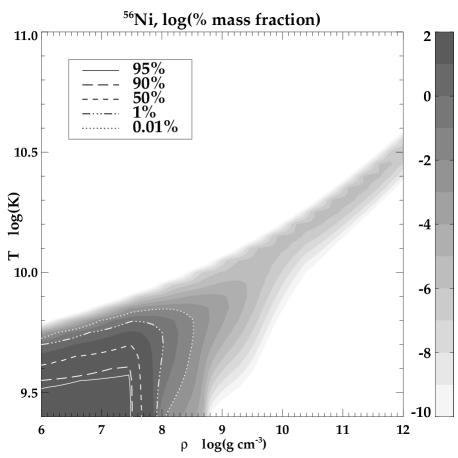
Figure 36: ⁵⁶Ni abundances in NSE, as percentages of relative mass fraction in the relevant $(\rho,T)$ phase space, with successive shades representing order of magnitude intervals in log(%).

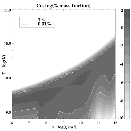
Figure 37: Co abundances (and see Fig. 36).

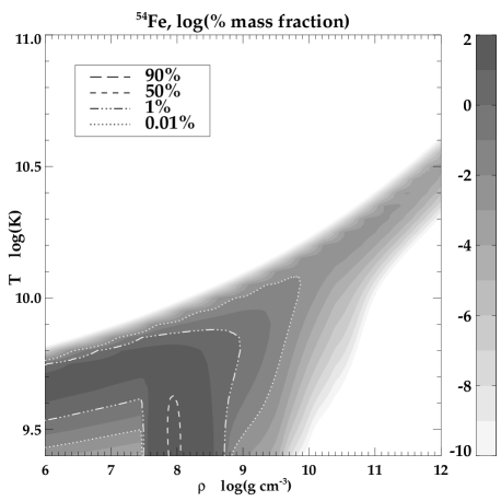
Figure 38: ⁵⁴Fe abundances (and see Fig. 36).

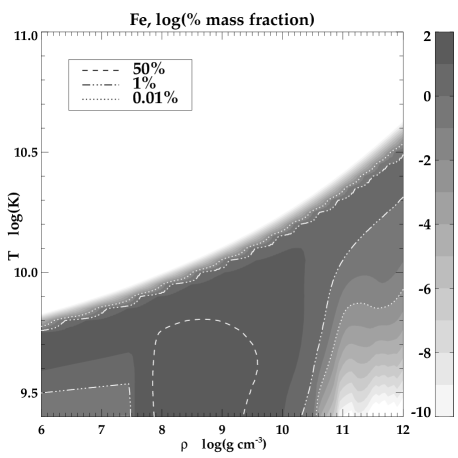
Figure 39: Fe abundances (and see Fig. 36).

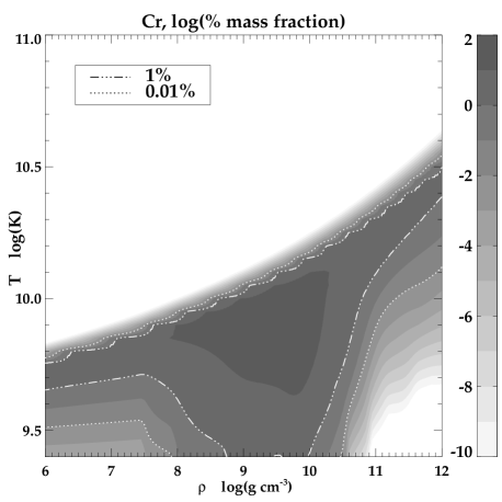
Figure 40: Cr abundances (and see Fig. 36).

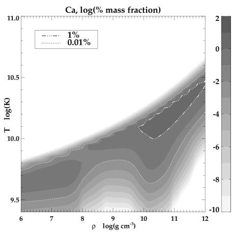
Figure 41: Ca abundances (and see Fig. 36).

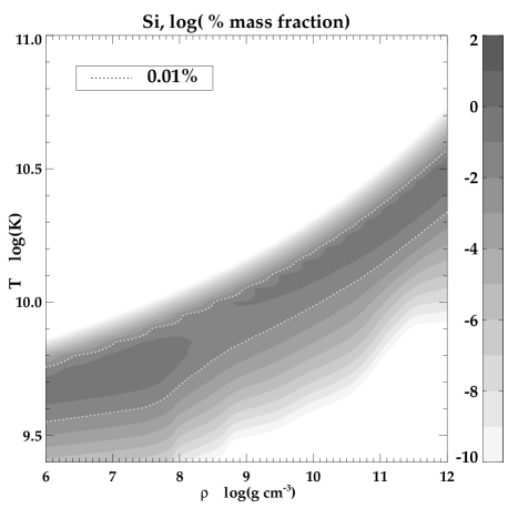
Figure 42: Si abundances (and see Fig. 36).

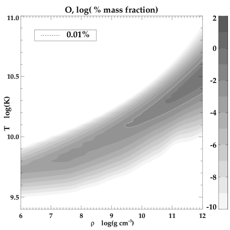
Figure 43: O abundances (and see Fig. 36).

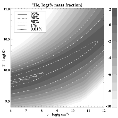
Figure 44: ⁴He abundances (and see Fig. 36).

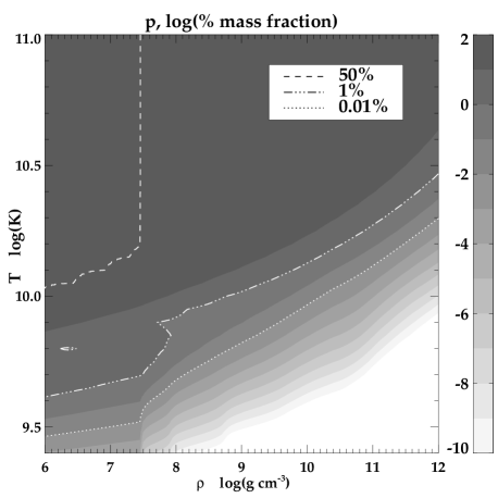
Figure 45: Proton abundances (and see Fig. 36).

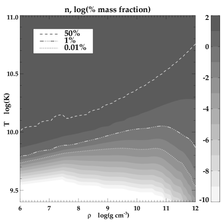
Figure 46: Neutron abundances (and see Fig. 36).

References

- Abramowicz et al. (1996) Abramowicz M. A., Beloborodov A. M., Chen X.-M., Igumenshchev I. V., 1996, A&A, 313, 334
- Artemova et al. (1996) Artemova I. V., Björnsson G., Novikov I. D., 1996, ApJ, 461, 565
- Balbus & Hawley (1991) Balbus S. A., Hawley J. F., 1991, ApJ, 376, 214
- Balsara (1995) Balsara D. S., 1995, Journal of Computational Physics, 121, 357
- Barnes & Hut (1986) Barnes J., Hut P., 1986, Nature, 324, 446
- Bate et al. (1995) Bate M. R., Bonnell I. A., Price N. M., 1995, MNRAS, 277, 362
- Birkl et al. (2007) Birkl R., Aloy M. A., Janka H.-T., Müller E., 2007, A&A, 463, 51
- Blandford & Znajek (1977) Blandford R. D., Znajek R. L., 1977, MNRAS, 179, 433
- Bodansky et al. (1968) Bodansky D., Clayton D. D., Fowler W. A., 1968, Physical Review Letters, 20, 161
- Bucciantini et al. (2009) Bucciantini N., Quataert E., Metzger B. D., Thompson T. A., Arons J., Del Zanna L., 2009, MNRAS, 396, 2038
- Campana et al. (2006) Campana S., Mangano V., Blustin A. J., et al., 2006, Nature, 442, 1008
- Chapman et al. (2009) Chapman R., Priddey R. S., Tanvir N. R., 2009, MNRAS, 395, 1515
- Chornock et al. (2010) Chornock R., Berger E., Levesque E. M., et al., 2010, ArXiv e-prints
- Colgate et al. (1993) Colgate S. A., Herant M. E., Benz W., 1993, Phys.Rep., 227, 157
- Fromang et al. (2004) Fromang S., Balbus S. A., De Villiers J.-P., 2004, ApJ, 616, 357
- Fromang et al. (2004) Fromang S., Balbus S. A., Terquem C., De Villiers J.-P., 2004, ApJ, 616, 364
- Fruchter et al. (2006) Fruchter A. S., Levan A. J., Strolger L., et al., 2006, Nature, 441, 463
- Fryer (1999) Fryer C. L., 1999, ApJ, 522, 413
- Fryer (2006) Fryer C. L., 2006, New Astronomy Review, 50, 492
- Fryer et al. (1996) Fryer C. L., Benz W., Herant M., 1996, ApJ, 460, 801
- Fryer & Heger (2005) Fryer C. L., Heger A., 2005, ApJ, 623, 302
- Galama et al. (1998) Galama T. J., Vreeswijk P. M., van Paradijs J., et al., 1998, Nature, 395, 670
- Gamezo et al. (2005) Gamezo V. N., Khokhlov A. M., Oran E. S., 2005, ApJ, 623, 337
- Gammie (2001) Gammie C. F., 2001, ApJ, 553, 174
- Garmany et al. (1980) Garmany C. D., Conti P. S., Massey P., 1980, ApJ, 242, 1063
- Gingold & Monaghan (1977) Gingold R. A., Monaghan J. J., 1977, MNRAS, 181, 375
- Goldreich & Lynden-Bell (1965) Goldreich P., Lynden-Bell D., 1965, MNRAS, 130, 97
- Hachisu et al. (1987) Hachisu I., Tohline J. E., Eriguchi Y., 1987, ApJ, 323, 592
- Haft et al. (1994) Haft M., Raffelt G., Weiss A., 1994, ApJ, 425, 222
- Hannestad & Raffelt (1998) Hannestad S., Raffelt G., 1998, ApJ, 507, 339
- Hix & Meyer (2006) Hix W. R., Meyer B. S., 2006, Nuclear Physics A, 777, 188
- Imamura et al. (2000) Imamura J. N., Durisen R. H., Pickett B. K., 2000, ApJ, 528, 946
- Itoh et al. (1996) Itoh N., Hayashi H., Nishikawa A., Kohyama Y., 1996, ApJS, 102, 411
- Janiuk et al. (2004) Janiuk A., Perna R., Di Matteo T., Czerny B., 2004, MNRAS, 355, 950
- Janka et al. (1999) Janka H.-T., Eberl T., Ruffert M., Fryer C. L., 1999, ApJ, 527, L39
- Jordan & Meyer (2004) Jordan IV G. C., Meyer B. S., 2004, ApJ, 617, L131
- Klebesadel et al. (1973) Klebesadel R. W., Strong I. B., Olson R. A., 1973, ApJ, 182, L85+
- Kobulnicky & Fryer (2007) Kobulnicky H. A., Fryer C. L., 2007, ApJ, 670, 747
- Kohri & Mineshige (2002) Kohri K., Mineshige S., 2002, ApJ, 577, 311
- Langer (1998) Langer N., 1998, A&A, 329, 551
- Langer et al. (1998) Langer N., Heger A., García-Segura G., 1998, in Schielicke R. E., ed., Reviews in Modern Astronomy Vol. 11 of Reviews in Modern Astronomy, Massive Stars: the Pre-Supernova Evolution of Internal and Circumstellar Structure. pp 57–+
- Le Floc’h et al. (2003) Le Floc’h E., Duc P.-A., Mirabel I. F., et al., 2003, A&A, 400, 499
- Lee et al. (2000) Lee H. K., Wijers R. A. M. J., Brown G. E., 2000, Phys.Rep., 325, 83
- Lee et al. (2005) Lee W. H., Ramirez-Ruiz E., Page D., 2005, ApJ, 632, 421
- Li (2000) Li L.-X., 2000, Phys.Rev.D, 61, 084016
- Liebendörfer (2005) Liebendörfer M., 2005, ApJ, 633, 1042
- Lopez-Camara et al. (2009) Lopez-Camara D., Lee W. H., Ramirez-Ruiz E., 2009, ApJ, 692, 804
- Lucy (1977) Lucy L. B., 1977, AJ, 82, 1013
- Masada et al. (2007) Masada Y., Kawanaka N., Sano T., Shibata K., 2007, ApJ, 663, 437
- Mazzali et al. (2006) Mazzali P. A., Deng J., Nomoto K., et al. 2006, Nature, 442, 1018
- Mazzali et al. (2005) Mazzali P. A., Kawabata K. S., Maeda K., et al., 2005, Science, 308, 1284
- Meyer et al. (1998) Meyer B. S., Krishnan T. D., Clayton D. D., 1998, ApJ, 498, 808
- Modjaz et al. (2008) Modjaz M., Kewley L., Kirshner R. P., et al., 2008, AJ, 135, 1136
- Monaghan (1997) Monaghan J. J., 1997, Journal of Computational Physics, 136, 298
- Mukhopadhyay (2002) Mukhopadhyay B., 2002, ApJ, 581, 427
- Mukhopadhyay & Misra (2003) Mukhopadhyay B., Misra R., 2003, ApJ, 582, 347
- Murray (1996) Murray J. R., 1996, MNRAS, 279, 402
- Nagataki (2009) Nagataki S., 2009, ApJ, 704, 937
- Nagataki et al. (2006) Nagataki S., Mizuta A., Sato K., 2006, ApJ, 647, 1255
- Nagataki et al. (2007) Nagataki S., Takahashi R., Mizuta A., Takiwaki T., 2007, ApJ, 659, 512
- Nakamura et al. (2001) Nakamura T., Mazzali P. A., Nomoto K., Iwamoto K., 2001, ApJ, 550, 991
- Narayan et al. (2001) Narayan R., Piran T., Kumar P., 2001, ApJ, 557, 949
- Nicotra (2006) Nicotra O. E., 2006, ArXiv Nuclear Theory e-prints
- Nomoto et al. (2007) Nomoto K., Tanaka M., Tominaga N., Maeda K., Mazzali P. A., 2007, ArXiv e-prints
- Nomoto et al. (2006) Nomoto K., Tominaga N., Tanaka M., Maeda K., Suzuki T., Deng J. S., Mazzali P. A., 2006, Nuovo Cimento B Serie, 121, 1207
- Novikov & Frolov (1989) Novikov I. D., Frolov V. P., 1989, Physics of black holes. Dordrecht, Netherlands, Kluwer Academic Publishers, 1989, 351 p. Translation.
- Paczyński (1990) Paczyński B., 1990, ApJ, 363, 218
- Paczyński & Wiita (1980) Paczyński B., Wiita P. J., 1980, A&A, 88, 23
- Pian et al. (2006) Pian E., Mazzali P. A., Masetti N., et al., 2006, Nature, 442, 1011
- Podsiadlowski et al. (1992) Podsiadlowski P., Joss P. C., Hsu J. J. L., 1992, ApJ, 391, 246
- Podsiadlowski et al. (2004) Podsiadlowski P., Mazzali P. A., Nomoto K., Lazzati D., Cappellaro E., 2004, ApJ, 607, L17
- Popham et al. (1999) Popham R., Woosley S. E., Fryer C., 1999, ApJ, 518, 356
- Proga et al. (2003) Proga D., MacFadyen A. I., Armitage P. J., Begelman M. C., 2003, ApJ, 599, L5
- Pruet et al. (2004) Pruet J., Thompson T. A., Hoffman R. D., 2004, ApJ, 606, 1006
- Pruet et al. (2003) Pruet J., Woosley S. E., Hoffman R. D., 2003, apj, 586, 1254
- Rice et al. (2003) Rice W. K. M., Armitage P. J., Bate M. R., Bonnell I. A., 2003, MNRAS, 339, 1025
- Ruffert & Janka (1998) Ruffert M., Janka H.-T., 1998, A&A, 338, 535
- Safronov (1960) Safronov V. S., 1960, Annales d’Astrophysique, 23, 979
- Seitenzahl et al. (2008) Seitenzahl I. R., Timmes F. X., Marin-Laflèche A., Brown E., Magkotsios G., Truran J., 2008, ApJ, 685, L129
- Setiawan et al. (2004) Setiawan S., Ruffert M., Janka H.-T., 2004, MNRAS, 352, 753
- Shakura & Sunyaev (1973) Shakura N. I., Sunyaev R. A., 1973, A&A, 24, 337
- Shapiro & Teukolsky (1983) Shapiro S. L., Teukolsky S. A., 1983, Black holes, white dwarfs, and neutron stars: The physics of compact objects. Research supported by the National Science Foundation. New York, Wiley-Interscience, 1983, 663 p.
- Shibata et al. (2007) Shibata M., Sekiguchi Y., Takahashi R., 2007, Progress of Theoretical Physics, 118, 257
- Spitzer (1965) Spitzer L., 1965, Physics of fully ionized gases. Interscience Tracts on Physics and Astronomy, New York: Interscience Publication, 1965, 2nd rev. ed.
- Springel (2005) Springel V., 2005, MNRAS, 364, 1105
- Stanek et al. (2003) Stanek K. Z., Matheson T., Garnavich P. M., et al., 2003, ApJ, 591, L17
- Starling et al. (2010) Starling R. L. C., Wiersema K., Levan A. J., et al., 2010, ArXiv e-prints
- Steinmetz (1996) Steinmetz M., 1996, MNRAS, 278, 1005
- Surman et al. (2006) Surman R., McLaughlin G. C., Hix W. R., 2006, ApJ, 643, 1057
- Tassoul (1978) Tassoul J.-L., 1978, Theory of rotating stars. Princeton Series in Astrophysics, Princeton: University Press, 1978
- Thompson (1994) Thompson C., 1994, MNRAS, 270, 480
- Thorne et al. (1986) Thorne K. S., Price R. H., MacDonald D. A., 1986, Black holes: The membrane paradigm. Black Holes: The Membrane Paradigm
- Timmes (1999) Timmes F. X., 1999, ApJS, 124, 241
- Toomre (1964) Toomre A., 1964, ApJ, 139, 1217
- Umeda & Nomoto (2008) Umeda H., Nomoto K., 2008, ApJ, 673, 1014
- Usov (1992) Usov V. V., 1992, Nature, 357, 472
- Valenti et al. (2008) Valenti S., Benetti S., Cappellaro E., et al., 2008, MNRAS, 383, 1485
- Wheeler et al. (2000) Wheeler J. C., Yi I., Höflich P., Wang L., 2000, ApJ, 537, 810
- Woosley (1993) Woosley S. E., 1993, ApJ, 405, 273
- Woosley & Baron (1992) Woosley S. E., Baron E., 1992, ApJ, 391, 228
- Zahn (1992) Zahn J., 1992, A&A, 265, 115