Nearby Supernova Rates from the Lick Observatory Supernova Search. II. The Observed Luminosity Functions and Fractions of Supernovae in a Complete Sample

Abstract

This is the second paper of a series in which we present new measurements of the observed rates of supernovae (SNe) in the local Universe, determined from the Lick Observatory Supernova Search (LOSS). In this paper, a complete SN sample is constructed, and the observed (uncorrected for host-galaxy extinction) luminosity functions (LFs) of SNe are derived. These LFs solve two issues that have plagued previous rate calculations for nearby SNe: the luminosity distribution of SNe and the host-galaxy extinction. We select a volume-limited sample of 175 SNe, collect photometry for every object, and fit a family of light curves to constrain the peak magnitudes and light-curve shapes. The volume-limited LFs show that they are not well represented by a Gaussian distribution. There are notable differences in the LFs for galaxies of different Hubble types (especially for SNe Ia). We derive the observed fractions for the different subclasses in a complete SN sample, and find significant fractions of SNe II-L (10%), IIb (12%), and IIn (9%) in the SN II sample. Furthermore, we derive the LFs and the observed fractions of different SN subclasses in a magnitude-limited survey with different observation intervals, and find that the LFs are enhanced at the high-luminosity end and appear more “standard” with smaller scatter, and that the LFs and fractions of SNe do not change significantly when the observation interval is shorter than 10 d. We also discuss the LFs in different galaxy sizes and inclinations, and for different SN subclasses. Some notable results are that there is not a strong correlation between the SN LFs and the host-galaxy size, but there might be a preference for SNe IIn to occur in small, late-type spiral galaxies. The LFs in different inclination bins do not provide strong evidence for extreme extinction in highly inclined galaxies, though the sample is still small. The LFs of different SN subclasses show significant differences. We also find that SNe Ibc and IIb come from more luminous galaxies than SNe II-P, while SNe IIn come from less luminous galaxies, suggesting a possible metallicity effect. The limitations and applications of our LFs are also discussed.

1 Introduction

The luminosity function (LF) is used to describe the distribution of intrinsic brightness for a particular type of celestial object, and it is always intimately connected to the physical processes leading to the formation of the object of interest. Specifically, the LF of supernovae (SNe), among the most luminous and exciting transients, will provide important information on their progenitor systems and their evolutionary paths. The intrinsic LF of core-collapse SNe (CC SNe, hereafter) can constrain the distribution of ways that massive stars die at different initial masses (Smith et al. 2011a), and that of SNe Ia can illuminate how accreting white dwarfs in the various binary systems result in a thermonuclear explosion. The observed LF of SNe will provide information on the extinction they experienced in their host galaxies and their immediate environments, thus giving further clues to their physical origins.

From an observational point of view, the LF of SNe is an important tool for calculating the completeness of a survey or a follow-up campaign in order to understand the involved selection biases, and for deriving meaningful SN rates. Knowledge of the SN LF will also provide guidance on the expected number and brightness distribution of SNe in several new large surveys (e.g., Pan-STARRS, Kaiser et al. 2002; Palomar Transient Factory, Law et al. 2009), which can be used to estimate and coordinate the necessary resources for the follow-up efforts.

Until now, however, we have had only limited knowledge on the LF of SNe. Many factors contribute to the difficulties in measuring the observed SN LF, with the most important being the completeness of finding all SNe in a survey and gathering follow-up photometry and spectroscopy. To study the intrinsic LF of SNe, we need further knowledge on how the SNe are extinguished in their host galaxies. There is some theoretical work on this (e.g., Hatano, Branch, & Deaton 1998; Riello & Patat 2005), but there are still considerable uncertainties in these models.

Many previous measurements of SN rates have adopted different strategies to derive the survey completeness and control time, highlighting the uncertainties caused by limited knowledge of the SN LF. Some adopted an average luminosity plus a Gaussian scatter for the SNe (e.g., Cappellaro et al. 1999 [C99, hereafter]; Hardin et al. 2000; Barris & Tonry 2006; Botticella et al. 2008), while others used information from a follow-up sample with unknown completeness and biases (e.g., Pain et al. 2002; Blanc et al. 2004; Sullivan et al. 2006; Dilday et al. 2008). Some treat the LFs as observed, while others consider them as intrinsic and apply additional extinction corrections. The host-galaxy extinction correction toward SNe, however, is another poorly known quantity. Some studies adopted an arbitrary functional form, such as the positive side of a Gaussian distribution (Neill et al. 2006; Poznanski et al. 2007), or an exponential function (Dilday et al. 2008), while others followed the aforementioned theoretical guidance by Hatano et al. (1998) and Riello & Patat (2005) (e.g., Barris & Tonry 2006; Botticella et al. 2008; Horesh et al. 2008).

In theory, the observed LF of SNe can be derived from either a volume- or magnitude-limited search. For a volume-limited survey, the key factor is to have information (type, luminosity, and light curve) for all of the SNe in the sample. For a magnitude-limited survey, it is important to have this information for all of the SNe and then correct for the different survey volumes of SNe having different brightnesses (e.g., Bazin et al. 2009). It is also important for a magnitude-limited survey to go fairly deep in order to sample the faint end of the LF. As discussed in detail by Leaman et al. (2011; hereafter, Paper I), there are nearly complete spectroscopic classifications for the SNe discovered in our Lick Observatory SN Search (LOSS) galaxies. This search goes fairly deep, with a small observation interval for many nearby galaxies, so a significant fraction of our survey is in the volume-limited regime. In particular, we identified that our survey may have almost full control for galaxies within 60 Mpc and 80 Mpc for CC SNe and SNe Ia, respectively. Here we attempt to construct a complete SN sample to derive the observed LF.

This paper is organised as follows. Section 2 describes the construction of the complete SN sample, including the adopted light curves, the collection and fitting of the photometry, and the completeness study for every SN. In §3 we present the observed LFs and fractions of SNe in a volume-limited survey, while §4 gives the results for a magnitude-limited survey. Section 5 discusses correlations of the LFs with the SN subtypes and host-galaxy properties, and possible limitations and caveats in our LFs. Our conclusions are summarised in §6. Throughout the study, we adopt the WMAP5 Hubble constant of $H_{0}=73$ km s^-1 Mpc^-1 (Spergel et al. 2007), consistent with the recent direct determination based on Cepheid variables and SNe Ia by Riess et al. (2009).

2 The Construction of a Complete SN Sample

2.1 The SNe in the Luminosity Function Sample

Paper I discussed the different subsamples of SNe in our analysis. We elect to construct a complete SN sample in the “season-nosmall” sample of SNe, consisting of SNe that were discovered “in season” but were not in small (major axis $<1^{\prime}$) early-type (E/S0) galaxies. There are considerable advantages of using in-season SNe to construct the LF; they were discovered young, so there are premaximum data to help constrain the peak magnitudes. We also limit the sample to the SNe discovered by the end of year 2006, in accordance with the reduction of our follow-up photometry database. The reason for the exclusion of SNe in small early-type galaxies is due to the uncertain detection efficiency (as discussed in Paper I) which results in an uncertain completeness correction (§2.5). As discussed in §5.5, only two SNe were excluded from the LF study because their host galaxies are small early-type galaxies, and their inclusion would have negligible effect on the LFs.

We use a cutoff distance of 80 Mpc for the SN Ia sample and 60 Mpc for SNe Ibc and II (see Paper I). In §2.5, we will compute the completeness of our survey for each SN selected in our LF sample. In total, we select 74 SNe Ia, 25 SNe Ibc, and 81 SNe II, for a grand total of 180 SNe. Table 1 lists some basic information on the SNe and their host galaxies (more details can be found in the galaxy and SN sample tables in Paper I). Five of the SNe (SNe 1999bw, 2000ch, 2001ac, 2002kg, and 2003gm) are so-called “SN impostors” — low-luminosity SNe IIn that are likely to be superoutbursts of luminous blue variable stars rather than genuine SNe (e.g., Van Dyk et al. 2000; Smith et al. 2011b); they are not considered further in this analysis, but will be discussed in a future paper.

We note that since our survey is conducted without using a filter, the images are most closely matched to the $R$ band (Li et al. 2003a). In the following several sections, we therefore focus our effort on deriving an $R$-band luminosity for the SNe. Some discussion of LFs in other passbands can be found in §5.5, and a full analysis of multi-colour LFs for SNe Ia will be presented elsewhere (Li et al. 2011b).

We also note that for all of the LF analysis, our photometry is corrected for the Galactic extinction adopted from Schlegel, Finkbeiner, & Davis (1998) to avoid additional scatter in the LF caused by the random Galactic extinction that the SNe suffered. Because of this, our LF is “pseudo-observed” and only the SN host-galaxy extinctions are not corrected. When applying our LF to a known direction in the Milky Way, the corresponding Galactic extinction should be applied to the luminosity of the LF SNe.

2.2 Light-Curve Families for the SNe

Different types of SNe exhibit a great degree of heterogeneity in their photometric behaviour (e.g., Barbon, Ciatti, & Rosino 1979; Leibundgut et al. 1991). Within a specific SN type, some homogeneity and correlations are observed, but no type can be well represented by a single light curve. Ideally, it would be good to have a well-observed light curve for every SN in the LF sample, but unfortunately this is not the case (see more details in §2.3). To quantify the light-curve shape distribution for our LF SNe, we construct a family of light curves for each type of SN from the literature and/or our own database of optical photometry.

2.2.1 Type Ia Supernovae

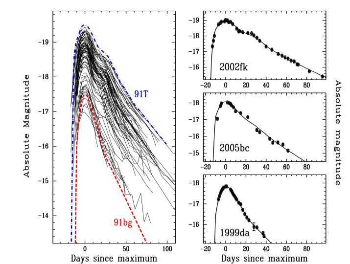
Figure 1: The light-curve fitting process for the SNe Ia. In the left panel, the solid lines are the observed $R$-band light curves in our photometry database (Ganeshalingam et al. 2010), while the smoothed light curves of SNe 1991T (dash-dotted line; Lira et al. 1998) and 1999by (dashed line, marked as “91bg”; Garnavich et al. 2004) are placed with an arbitrary peak absolute magnitude of $-19.5$ and $-17.5$ mag, respectively. A family of 21 light curves is interpolated between these two extreme curves, and is used to fit the individual objects shown in the right-hand panels.

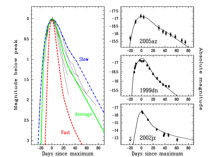
Figure 2: Same as Figure 1 but for the SNe Ibc. A family of three light curves (fast, average, and slow) is constructed (see text for details), and is used to fit the individual objects shown in the right panels.

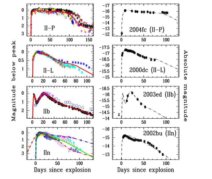
Figure 3: Same as Figure 1 but for the SNe II. A single average light curve is constructed for the subclasses of SNe II-P, II-L, and IIb, while three light curves (fast, average, and slow) are for SNe IIn. The fast SN IIn light curve (dash-dotted line) is plotted relative to days since maximum brightness. The right panels show an example fit for each subclass.

With a few exceptions (e.g., Li et al. 2001a, 2003b; Howell et al. 2006; Foley et al. 2010b), SNe Ia are generally thought to form a one-parameter family, with the fast-declining SNe also being subluminous, and slow decliners being luminous (e.g., Phillips 1993). In the left panel of Figure 1, we plot the $R$-band light curves of a sample of 83 well-observed SNe Ia in the LOSS photometry database (solid lines; Ganeshalingam et al. 2010). The time axis show the number of days since $R$-band maximum, and the light curves are plotted on an absolute magnitude scale, after the SNe were corrected for Galactic extinction. The distances toward the SNe are calculated from the recession velocities corrected for infall of the Local Group toward the Virgo cluster. Also overplotted are the light curves of SN 1991T (dash-dotted line, from Lira et al. 1998) and the well-observed SN 1991bg-like object SN 1999by (dashed line, from Garnavich et al. 2004), arbitrarily shifted to absolute magnitudes of $-19.5$ and $-17.5$, respectively. The published light curves of SNe 1991T and 1999by have been smoothed with a spline function (as are all of the other template SN light curves shown in Figures 1–3). As can be seen, the light curves of SNe 1991T and 1999by nearly encompass all of the observed SNe Ia in our photometry database. We interpolate between the two curves to create 21 light curves (so each curve has a different shoulder prominence and peak absolute magnitude), and use them as the light-curve family for SNe Ia. While our construction of the light-curve family for SNe Ia is not drastically different from previous approaches (e.g., the application of a stretch factor to a template light curve), we need to use interpolation (rather than stretch) during the construction to deal with the presence or absence of the shoulder feature in the $R$-band light curves.

A few SNe in the SN Ia LF sample belong to the so-called “SN 2002cx-like objects” (Filippenko 2003; Li et al. 2003b; Jha et al. 2006b; Phillips et al. 2007), which show distinct differences from the rest of the SN Ia family Recently, their SN Ia nature has been questioned (Valenti et al. 2009; but see Foley et al. 2009b, 2010a). We constructed a template light curve from SN 2005hk (Phillips et al. 2007), a well-observed SN 2002cx-like object.

2.2.2 Type Ibc Supernovae

Compared to the wealth of published photometry for SNe Ia, the Type Ibc SNe are not well observed. It is unclear whether they can be described by a one-parameter family. Some studies suggest that they can be broadly classified into two bins (e.g., Clocchiatti & Wheeler 1997): the fast-evolving and the slow-evolving subclasses. In the left panel of Figure 2, we plot the $R$-band light curves of 8 SNe Ibc from our unpublished photometry database. There is no fast-evolving object among these 8 SNe, so we adopted the photometry of SN 1994I (dashed line, Richmond et al. 1996), a well-observed object in this subclass. We have an excellent light curve for the slow-evolving SN Ibc 2004dk (dash-dotted line) in our own photometry database which we use as a template. For the rest of the SNe Ibc, we construct an average light curve (solid line). The late-time behaviour of the average SN Ibc is not well constrained by our sample, so we utilised an additional sample of SNe Ibc from Modjaz (2007). This family of three light curves is used to fit the majority of the SNe Ibc in our LF sample (without any stretching or interpolating).

For the so-called “Ca-rich” subclass of peculiar SNe Ibc, we chose the light curve of SN 2005E (Perets et al. 2010). Unfortunately, there are no premaximum data for SN 2005E, so we adopted that portion from the average SN Ibc light curve. This light curve is not shown in Figure 2. The “SN Ibc-pec” subclass also contains SN 2003id (Singer et al. 2003; Hamuy & Roth 2003), the broad-lined SN Ic 2002ap (Foley et al. 2003; see more discussion in §3.2), and SN 2004bm (§3.2). The photometric behaviours of these SNe Ibc-pec are all reasonably represented by the average SN Ibc light curve.

2.2.3 Type II Supernovae

The photometric behaviour of SNe II is the most heterogeneous among all SN types, and they can be divided into a few main photometric and spectroscopic subclasses. SNe II-P have a prominent “plateau” phase in their light curves, while SNe II-L decline linearly (in magnitudes) after maximum brightness. SNe IIb show prominent hydrogen Balmer lines in their early-time spectra, but morph into SNe Ib at late times. In addition, the prototypical SN IIb 1993J showed a double-peaked light curve (Richmond et al. 1994), with a very early first peak, which we now think is most likely due to black-body emission from the expanding and cooling shock-heated stellar envelope (e.g., Waxman et al. 2007), and the regular Ni⁵⁶-powered main maximum. This double-peak light curve behaviour has most recently also been seen in the Type Ib SN 2008D (Soderberg et al. 2008; Modjaz et al. 2009). While it is not clear how common and pronounced the early first peak is among other SNe IIb besides the well-studied SN 1993J (e.g., Chevalier & Soderberg 2009), we use the smoothed light curve of SN 1993J as the light-curve template for SN IIb. SNe IIn show a strong “narrow” (actually, generally an intermediate width of $\sim 1000$ km s^-1) component to their hydrogen Balmer lines and a wide variety of light curves. See Filippenko (1997) for a detailed discussion of the classifications of these different subtypes.

The distinction between a SN II-P and a SN II-L in terms of photometric evolution is not well documented in the literature, especially in the $R$ band. The collection of light curves for the SNe II-L in Barbon et al. (1979) and Young & Branch (1989) are all in the $B$ band. For our application, we define a SN II as being a SN II-L if it declines by more than 0.5 mag in the $R$ band during the first 50 d after explosion.

The left panels of Figure 3 show how the light curves of the SNe II are constructed. The top panels show the light curves of 15 SNe II-P (dots) in our photometry database that have been published by Poznanski et al. (2009). As seen here, and also noted by Hamuy (2003), SNe II-P vary in the durations of their plateau phase. We use the average light curve (solid line) as the template. The second panel shows the light curves of 5 SNe II-L in our unpublished photometry database; again, an average is derived as the template. Due to the lack of data, the late-time behaviour of the SN II-L template is not well constrained and may have relatively large uncertainty. The third panel shows the light curves of 3 SNe IIb: the prototypical SN IIb 1993J (Richmond et al. 1994), and the unfiltered light curves of SNe 2003gu and 2005em from our photometry database. We use the smoothed light curve of SN 1993J as the template. The rising portion of the first peak is not well observed, so our manual construction is quite arbitrary after considering the earliest nondetections and detections (e.g., Wheeler et al. 1993).

The bottom-left panel of Figure 3 shows the construction of the template light curves for SNe IIn. Eight well-observed SNe IIn from our photometry database are plotted, displaying a great degree of heterogeneity. This mirrors what has been reported in the literature about the photometric behaviour of this class of objects: SNe IIn can range from very slowly evolving objects such as SN 1988Z (e.g., Turatto et al. 1993) and SN 1995G (Pastorello et al. 2002), to more typical objects like SN 1994W (Sollerman, Cumming, & Lundqvist 1998), to very rapidly evolving objects such as SN 1998S (Fassia et al. 2000). We use the light curve of SN 1998S (dash-dotted line) as the template of a fast-declining SN IIn, that of SN 2003dv (dashed line) as the template for a slow-evolving SN IIn, and the average of the remaining seven objects (solid line) for the average SN IIn.

2.3 Photometry of the LF SNe

It is important to collect photometry for every SN in the LF sample to study the light-curve shape and derive the peak absolute magnitude; otherwise, the sample will not be complete. Since our unfiltered survey images are most closely matched to the $R$ band, we use the follow-up $R$-band photometry for the SNe whenever possible. This is because the images taken during the follow-up campaigns have a higher cadence (every 1–2 d near maximum light, every 2–4 d thereafter) than the unfiltered images taken during the SN search. Moreover, accurate photometric calibrations for the fields have been obtained with the 0.76 m Katzman Automatic Imaging Telescope (KAIT) and the 1.0 m Nickel telescope at Lick Observatory on many photometric nights. The reduction details are described by Ganeshalingam et al. (2010), where the filtered photometry for the SNe Ia is also provided. An important step in the reduction is the careful removal of the host-galaxy contamination in the SN flux by subtracting a template image taken long after the SN has faded.

For SNe Ia, 62 of the 74 SNe (84%) in the LF sample have filtered follow-up photometry. This large fraction is due to the combined effect of the luminous nature of SNe Ia relative to most other SNe, the early discovery, and our emphasis on studying them. For several SNe (details listed in Table 3), the follow-up photometry is adopted from Jha et al. (2006a; hereafter “CfA-2”) and Hicken et al. (2009; hereafter “CfA-3”). Only 7 out of the 25 SNe Ibc (28%) have follow-up photometry, and for SNe II the corresponding numbers are 18 out of 76 (24%).

For the SNe that do not have filtered follow-up photometry, we derive unfiltered light curves from the SN search images. As discussed in Paper I, our search has a relatively short observation interval, so we cover the photometric evolution of the SNe rather well. This is especially true for the SNe in the LF sample, as their host galaxies are mostly in the sample that has a designed observational interval of every 5 d. To reduce the unfiltered images, a high signal-to-noise ratio template image without the SN is selected. The host-galaxy contamination is then cleanly removed after image subtraction, similar to what is done in the follow-up data reduction described by Ganeshalingam et al. (2010). For photometric calibration, we use the red magnitudes for the stars in the SN fields in the USNO B1 catalog (Monet et al. 2003). Although the accuracy of this calibration is only $\sim 0.2$–0.3 mag for an individual star, there are usually more than 10 stars available in each field, so the uncertainty due to calibration is $<0.1$ mag.

We have good unfiltered light curves for a majority of the SNe without follow-up filtered photometry. However, for a small fraction of the SNe (13 out of 175, or 7%), our photometric coverage is relatively poor. Some of them were discovered near the end of an observing season, so the search images did not cover the whole period around maximum light. A few others are faint and the search images do not go deep enough to yield a constraint on the light-curve shape. The majority of them, however, are due to a combination of bad weather and relatively low cadence. For two objects (SNe 2005W and 2006dy in Table 3), we adopted the photometry measured by amateur astronomers posted on SNWeb, with good coverage around maximum light. For the other SNe, we pool all of the information on the SNe together (discovery magnitude, spectral identification and age estimate, unfiltered and filtered photometry in our database and published elsewhere) and constrain the light curves as much as possible. Some of them still have large uncertainties, as reflected in the error bars for their peak magnitudes. We also use the average light curves according to their types for these poorly observed SNe.

2.4 The Light-Curve Fitting Method

We use a $\chi^{2}$-minimizing technique to fit light curves constructed in §2.2 to the photometry collected in §2.3, to determine the light-curve shape and peak magnitude for each SN, as demonstrated in the right-hand panels of Figures 1 to 3. Because we attempt to use a small set of light curves to describe the complicated observed variety of photometric behaviour for the different types of SNe, the fit to the data is not always perfect, and the reduced $\chi^{2}$ of the fit can be several times larger than unity. Whenever possible, the peak magnitudes are directly measured from a spline fit to the data near maximum brightness rather than measured from the light-curve fit. As noted by Cappellaro et al. (1993), the control-time calculation for a SN search is more sensitive to the adopted peak luminosity of a SN than to its light-curve shape. The imperfections in the light-curve fits also have a chance to cancel each other out when many SNe are combined in the LF. So, the uncertainty in the light-curve shape likely has little effect on the final control-time calculation.

We visually check the fits, especially the ones with relatively large reduced $\chi^{2}$, to make sure they are a reasonable representation of the data, and if not, to determine the possible causes. By doing this, we identified two misclassifications in the LF SNe, SNe 2002au and 2006P, as detailed in Paper I. Both SNe were originally classified as possible SNe Ia, but their light-curve fits suggest SN IIb and SN Ic, respectively. An analysis of their observed spectra confirms the suggestion from the light-curve fit. This exercise partly validates our constructed light-curve families and the light-curve fitting process.

The peak apparent magnitudes measured for the SNe are converted to absolute magnitudes using distances measured from the recession velocities corrected for the infall of the Local Group toward the Virgo Cluster. To account for peculiar velocities in the local flow, we adopt 300 km s^-1 as the uncertainty for the recession velocities. The uncertainties of the absolute magnitudes include the photometry measurement error, the light-curve fit uncertainty, and the distance uncertainty added in quadrature. Columns 3 and 4 of Tables 3–5 list the results for different types of SNe.

2.5 The Completeness of Each LF SN

It is important to correct for possible incompleteness of the SNe in the LF sample. For a particular SN in the LF sample, the peak absolute magnitude and light-curve shape are given in §2.4. With this information, we can calculate the control time for this SN for the LOSS galaxies in the “full-nosmall” sample (the control galaxy sample for the LF SNe; see Paper I) using their monitoring history log files [see Paper III (Li et al. 2011a) for details of the control-time calculation]. The completeness of of our search to a particular SN at a given distance is then defined as the sum of the control time of that particular SN for all of the galaxies within that distance divided by the sum of the observing season time for these galaxies. To correct a SN to 100% completeness within the cutoff distance of the LF sample, one just needs to use the reciprocal of the completeness as the corrected number for the SN.

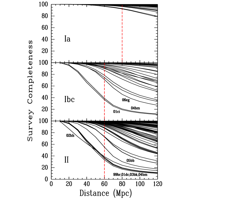
Figure 4: The completeness of each SN in the LF sample in our SN search. The completeness is defined as the ratio of the total control time divided by the total season time. Some notable SNe are marked. The dashed lines mark the cutoff distances within which the LF samples are constructed.

Figure 4 shows the completeness measurements for the SNe in the LF sample. Each curve represents a SN, and some of the notable SNe are labeled. The vertical dashed lines indicate the cutoff distance where the sample is constructed. The top panel shows the completeness measurements for the SNe Ia. We achieved a completeness higher than 98% for all of the SNe Ia because of their extreme luminosity at peak. The total number of SNe after correction for the incompleteness is 74.70, only a 1% change from the input number of 74. The middle and bottom panels show the completeness measurements for the CC SNe. The majority of the SNe have completeness higher than 80% at the cutoff distance of 60 Mpc, but a few of them have relatively low completeness due to their extremely low luminosity. For example, SN 1999br (Pastorello et al. 2004) is an intrinsically faint SN II-P, while SN 2002hh (Pozzo et al. 2006) is a highly reddened SN II-P in the nearby galaxy NGC 6946.

The corrected number for each SN in the LF function after applying the completeness correction factor (hereafter CCF) is listed in Column 7 of Tables 3–5. The total corrected number of SNe Ibc is 28.86, an 18% increase compared to the input number of 24.5. For SNe II, the corrected number of 88.50 is a 16% increase over the input number of 76.5. We see that even though our search does not have full control for all of the SNe within the cutoff distance of the LF sample, the correction to 100% completeness is small and thus our LF should not suffer large uncertainties (see additional discussion in §5).

3 The Volume-Limited Sample: LFs and Fractions of SN Types

3.1 The Observed LFs of SNe

The “pseudo-observed” LFs of the SNe (corrected for Milky Way extinction but not host-galaxy extinction) are listed in Tables 3–5 for the different types. The following information is included for each SN: the subtype, the absolute magnitude and its uncertainty, the distance of the SN, the Hubble type, inclination, and mass of its host galaxy, the corrected LF number for a volume-limited sample, the corrected LF number for a magnitude-limited sample (discussed in the next section), the light-curve shape of the SN, the source of the photometry, and additional comments. Each SN constitutes a discrete point in the LF, with its own peak absolute magnitude, light-curve shape, and number contribution to the total LF.

Although it would be ideal to construct a LF for galaxies of every Hubble type, it is impractical with the relatively small total number of SNe in the LF sample. Instead, the SNe are grouped into two broad bins for each SN type: E–Sa and Sb–Irr for SNe Ia, S0–Sbc and Sc–Irr for the CC SNe. The split of the Hubble types is motivated by an attempt to include reasonable numbers of SNe in each LF, rather than by physics. For example, one may argue that splitting the SNe Ia by E–S0 (early-type) and Sa–Irr (late-type) galaxies may be more physically based, but then the E–S0 bin would suffer more from small-number statistics. As discussed in Paper III, the exact manner in which the SN Ia LF is split has negligible effect on the final derived SN Ia rates.

To study the statistical properties of the LFs, we use histograms to show their luminosity distribution, but we emphasise that the LFs should be used as discrete points when calculating the control time for a survey. We also use the Kolmogorov-Smirnov (K-S) test exclusively to study whether two groups of objects come from the same population (in terms of absolute magnitudes only). We note that the histograms show the distributions of the corrected numbers of the LFs; thus, the number of SNe in each bin does not correctly reflect Poisson statistics. Since the CCFs are always greater than 1, the Poisson uncertainty of each bin is always larger than that calculated directly from the number of SNe in the bin. For example, if one bin has a single SN with a CCF of 2.0, the number of SNe in the bin with proper Poisson errors is $2.0\times 1.0^{+2.29}_{-0.83}=2.0^{+4.58}_{-1.66}$ (i.e., the error is 2.0 times the Poisson error of 1.0 SN; Gehrels 1986), rather than $2.0^{+2.63}_{-1.29}$ (i.e., the Poisson error calculated directly from 2.0 SNe). In the same vein, the K-S tests are also somewhat compromised due to the deviation from Poisson statistics. Fortunately, the CCFs are close to 1.0 for all of the SNe in the LFs except for the objects fainter than $-15$ mag. In our subsequent discussions, all significant K-S test results will be scrutinised by including/excluding the least luminous objects in the LFs.

To properly consider the effect of the uncertainties of the LF SN absolute magnitudes on the K-S test results, we run a Monte Carlo simulation 1000 times to sample the absolute magnitudes according to their Gaussian errors, and study the scatter of the resultant cumulative distribution functions (CDFs; also called cumulative fractions) and the probabilities of the two samples coming from the same population.

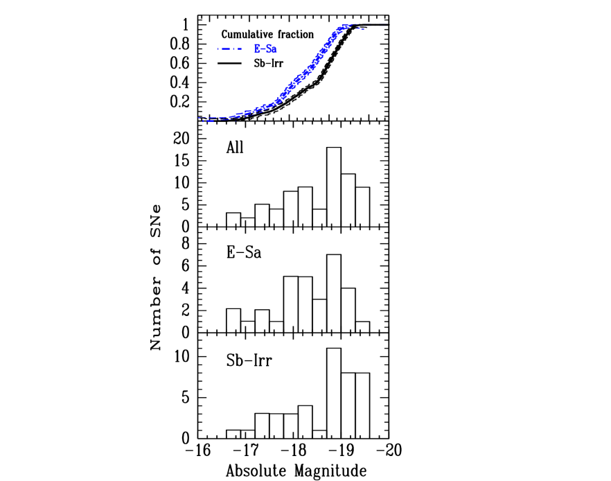
Figure 5: The pseudo-observed LFs of SNe Ia. The top panel shows the cumulative fractions for the LFs in two different galaxy Hubble-type bins (E–Sa and Sb–Irr). The dashed lines show the $1\sigma$ spread in the cumulative fractions considering only the uncertainties in the peak absolute magnitudes. The bottom panels show the LFs in all, E–Sa, and Sb–Irr galaxies.

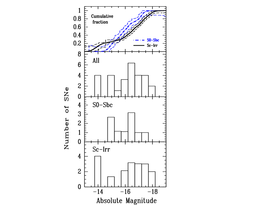
Figure 6: Same as Figure 5 but for SNe Ibc. The galaxies are split into S0–Sbc and Sc–Irr bins.

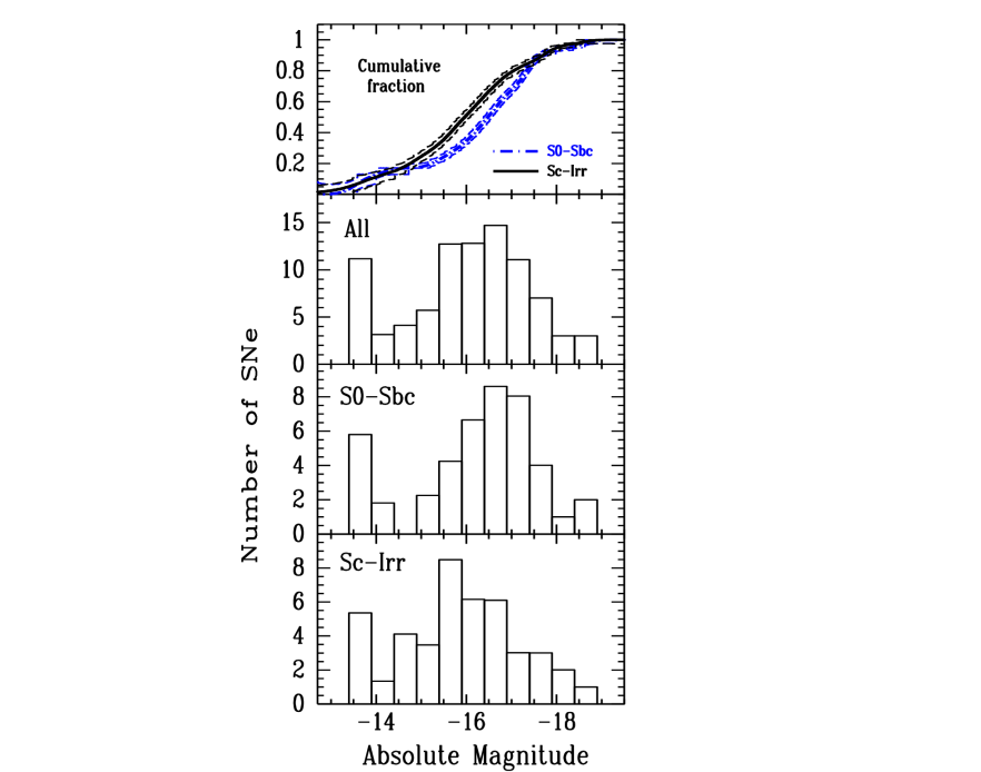
Figure 7: Same as Figure 6 but for SNe II.

Figures 5–7 display the histograms for the LFs of SNe Ia, Ibc, and II, respectively. The second panel of each figure shows the distribution for the whole LF sample. We note that while a Gaussian distribution is an acceptable but not ideal description for the LFs of SNe Ibc and II, it is a rather poor description for the LF of SNe Ia. The average absolute magnitudes are $-18.49\pm 0.09$ (with a $1\sigma$ dispersion of 0.76), $-16.09\pm 0.23$ ($\sigma=1.24$), and $-16.05\pm 0.15$ ($\sigma=1.37$) for the SNe Ia, Ibc, and II, respectively. These numbers, together with the average absolute magnitudes for several other combinations, are listed in Table 6.

Richardson et al. (2002) did an extensive comparative study of the peak absolute magnitude distribution for the SN discoveries compiled in the Asiago SN Catalog (Barbon, Cappellaro, & Turatto 1989; Barbon et al. 1999). Their study was done in the $B$ band, although they did not distinguish among the different photometric bands for some SNe. They derived an absolute magnitude (without extinction corrections, and converting to $H_{0}=73$ km s^-1 Mpc^-1 used in our study) of $-18.73\pm 0.07$ ($\sigma=0.76$) for normal SNe Ia, $-17.49\pm 0.30$ ($\sigma=1.29$) for SNe Ibc, and $-16.18\pm 0.23$ ($\sigma=1.23$) for SNe II-P. We note the significant difference compared with our result for the average peak absolute magnitudes of SNe Ibc: the Richardson et al. sample suggests a much brighter magnitude relative to SNe Ia and II. As Richardson et al. noted, there are considerable observational biases in their observed SN sample and the completeness is unknown. In particular, the SN Ibc subclass may be more heavily biased in the observed sample due to its low peak luminosity (relative to SNe Ia) and fast photometric evolution (relative to SNe II-P).

Figure 5 shows the histograms for the LFs of SNe Ia in different galaxy bins (the two lower panels). The LF in E–Sa galaxies shows an apparent difference from the LF in Sb–Irr galaxies, with only a $8.5^{+10.3}_{-5.0}$% probability that they come from the same population (the cumulative fractions and their 1$\sigma$ scatters are plotted in the top panel). This is likely caused by the observed preference of different subclasses of SNe Ia in host galaxies of different Hubble types: the subluminous SN 1991bg-like objects in early-type galaxies and the overluminous SN 1991T-like objects in spiral galaxies (e.g., Della Valle & Livio 1994; Hamuy et al. 1996; Howell 2001).

Figure 6 shows the histograms for the LFs of SNe Ibc in different galaxy bins (the two lower panels). The K-S test does not provide evidence for a significant difference between the two LFs: the SNe come from the same population at a $46.3^{+23.0}_{-21.2}$% probability. SNe Ibc in the early-type spiral galaxies appear on average marginally fainter (averaging $-15.98\pm 0.26$ mag; $\sigma=0.83$ mag) than their counterparts in the late-type spirals (average of $-16.15\pm 0.33$ mag; $\sigma=1.43$ mag).

Figure 7 shows the histograms for the LFs of SNe II in different galaxy bins (the two lower panels); there is a marginal difference, with a $21.0^{+19.5}_{-10.7}$% probability that they come from the same population. Contrary to the trend shown by the SNe Ibc, in the early-type spirals SNe II are marginally brighter (average of $-16.22\pm 0.21$ mag; $\sigma=1.39$ mag) than their counterparts in the late-type spirals, which average $-15.88\pm 0.20$ mag ($\sigma=1.34$ mag). The significance of the difference between the two LFs is not dramatically affected by the objects fainter than $-15$ mag: when they are excluded from the statistics, the two LFs come from the same population with a $28.0^{+27.7}_{-16.0}$% probability.

It is generally expected that SNe occurring in late-type galaxies should on average experience more extinction than those in early-type galaxies because of a dustier environment. This fact should be taken into account when translating differences in the observed LFs in various Hubble types into differences in the intrinsic LFs. For example, SNe Ia that occurred in Sc–Irr galaxies should be intrinsically brighter than SNe Ia in E–Sa galaxies by a bigger margin than is shown in Figure 5.

In a recent paper, Bazin et al. (2009) derived an overall core-collapse SN LF from the Supernova Legacy Survey (SNLS). A comparison between our combined SN Ibc and SN II LF and that reported by Bazin et al. shows excellent agreement (J. Rich, 2010, private communication).

3.2 The Observed Fractions of SNe

In the process of analysing the LF SNe in detail, we are able to put them into different subclass bins. For SNe Ia, the light-curve fitting sequence from 1 to 21 is a loose luminosity indicator, as we demonstrate in a forthcoming paper (Li et al. 2011b). Moreover, the SNe are categorised into several subclasses: normal SNe Ia with normal expansion velocities (“IaN” in Table 3 and hereafter), normal SNe Ia with high expansion velocities (“IaHV,” see Wang et al. 2009 for our definition of this subclass), SN 1991bg-like objects (“Ia-91bg”; Filippenko et al. 1992b; Leibundgut et al. 1993), SN 1991T-like objects (“Ia-91T”; Filippenko et al. 1992a; Phillips et al. 1992), and SN 2002cx-like objects (“Ia-02cx”; Filippenko 2003; Li et al. 2003b; Jha et al. 2006b; Phillips et al. 2007). This classification is based on the information published in the IAU Circulars and/or analysis of the spectra in our spectral database (Silverman et al. 2011). As discussed by Li et al. (2001b), there is a significant “age bias” for SN 1991T-like objects, caused by the fact that such objects can only be easily identified with spectra taken prior to or near maximum brightness. Because of this, the fraction of SN 1991T-like objects should be regarded as a lower limit in this study. As discussed by Wang et al. (2009), a spectrum (or expansion-velocity measurement) within a week around maximum brightness is required to classify a normal SN Ia into the “IaN” or “IaHV” subclasses. Fortunately, we were able to secure such information for all of the SNe Ia in our LF sample.

For SNe Ibc, both the fast- and slow-evolving SNe are relatively rare (10% for each subclass), but this conclusion is hampered by the relatively large fraction of SNe Ibc that are either peculiar or have poor light-curve coverage. We put the SNe Ibc into three subclasses: SN Ib, SN Ic, or peculiar Ibc or Ic (“Ibc-pec” or “Ic-pec,” which we consider as the same subclass). We note that in general, there is considerable uncertainty in classifying SNe Ibc into these subclasses. Sometimes the SNe are simply reported as “SN Ibc” in the IAU Circulars without a more specific subclass. Other times, a SN Ib would only develop strong He I lines after a few weeks, so it might be misclassified as a SN Ic from an early-time spectrum. The differences in the spectra of the different subclasses also become subtle when the SNe are in the nebular phase. Although there are spectra for 21 out of the 25 LF SNe Ibc in our spectral database, and the other 4 SNe were classified in IAU Circulars by experienced observers, we do not have a good series of spectra for every SN in the sample to check for a possible SN Ic to SN Ib transition, so the fraction of SNe Ic should be regarded as an upper limit in this study.

We attempt to place the SNe II into four subclasses: II-P, II-L, IIb, or IIn. For this purpose, SNe IIn can often be easily distinguished from the others because of their unique spectral features (a prominent narrow or intermediate-width emission component in the hydrogen Balmer lines), although in rare cases a SN IIn can spectroscopically evolve into a regular SN II (e.g., SN 2005gl, Gal-Yam et al. 2007). It is difficult to distinguish between the other three subclasses based on their spectra alone. First, the defining features or spectral evolution have not been established to distinguish a SN II-P from a SN II-L. Second, even though a SN IIb can be identified from its early resemblance to a SN II and late metamorphosis into a SN Ib, it is not clear whether an early SN II will turn out to be a SN IIb unless we have good spectroscopic coverage for every SN II. Fortunately, these three subclasses have rather different photometric behaviour: SNe II-P have a prominent plateau phase, SNe II-L have a linear decline (in magnitudes) after maximum, and SNe IIb have a double-peaked light curve (Figure 3). Consequently, for the majority of SNe our light-curve fitting process reports a strong preference for a certain subtype. For a few SNe with poor light-curve coverage, the data can be fit by more than one template light curve, and we assign equal fractional weights to the subclasses that provide a satisfactory fit.

One surprising result from the light-curve fitting process is a possible high fraction of SNe IIb in the SN II sample. Following identification of the first known SN IIb, SN 1987K (Filippenko 1988), detailed studies of only a few SNe IIb have been published in the literature. SN 1993J, the prototypical SN IIb in the nearby galaxy M81, has been extensively studied (e.g., Matheson et al. 2000, and references therein). Another SN IIb, SN 1996cb, was studied by Qiu et al. (1999). With the help of the “Supernova Identification code” (SNID; Blondin & Tonry 2007), some recent SNe have been classified as SN IIb. The fraction of SN IIb within the family of SNe II is very uncertain, but generally considered to be relatively small.

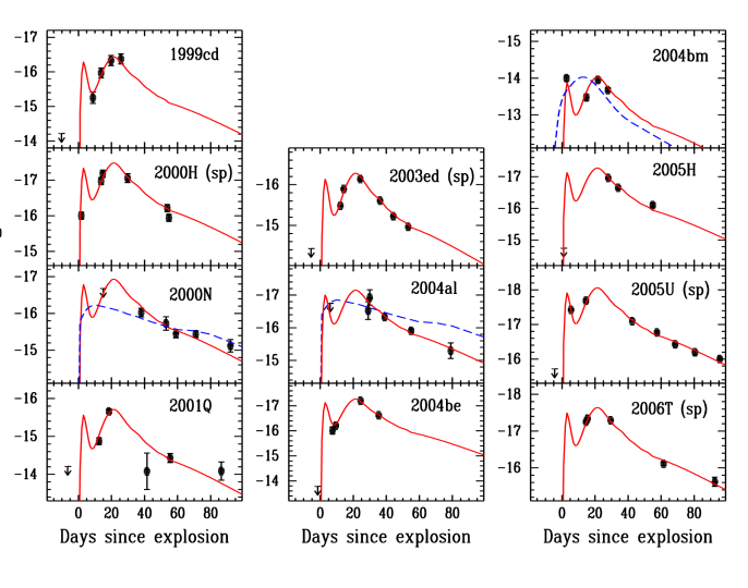
Figure 8: Possible SNe IIb in the LF sample. All of these objects were spectroscopically classified as SNe II based on the presence of hydrogen lines, but their light curves are best fit with a SN IIb template. The SNe labeled with “(sp)” were also spectroscopically confirmed as SNe IIb. The dashed lines are the fits with template light curves of SNe II-L (for SNe 2000N and 2004al) and SNe Ibc (for SN 2004bm). See text in §3.2 for more details.

Figure 8 shows all possible SNe IIb in our LF sample. Two of the objects, SNe 2000N and 2004al, can be fit with both a SN IIb and a SN II-L, so they are assigned 0.5 for each subclass. Foley et al. (2004) classified SN 2004bm as a probable SN Ic based on a low-quality spectrum. The light curve, though with only four points, shows a distinct dip that is reminiscent of a SN IIb. Reanalysis of the spectrum does not provide a confident classification for the SN, so we assign 0.5 for both IIb and Ibc-pec. The light curve of SN 2005H is rather poor. The photometric behaviours of the other seven SNe are best matched by the template SN IIb light curve. Considering that our template light curves are only an average of the observations, it is conceivable that a few of these SNe can be fit by some variations of SNe II-L (these SNe are clearly not SNe II-P, and their spectra do not show narrow emission components so they are also not SNe IIn); hence, the list of SNe in Figure 8 should be considered as an upper limit to possible SNe IIb in the LF sample. We also note that for four of our SN IIb candidates, there is spectroscopic confirmation of our classification: SN 2000H (Benetti et al. 2000), SN 2003ed (Leonard, Chornock, & Filippenko 2003), SN 2005U (Leonard & Cenko 2005), and SN 2006T (Blondin et al. 2006). We consider the SN IIb classification for these four objects to be solid, but for the rest of the SNe, we do not have spectra to corroborate the SN IIb classification from the light curves. Overall, we have four solid (5% of all the SNe II), or up to 9 possible (12% of all the SNe II), SNe IIb in our LF sample.

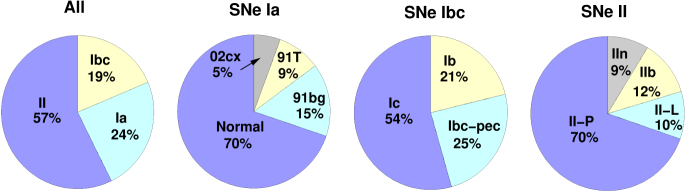
Figure 9: The observed fractions of the subclasses of SNe in a volume-limited sample, illustrated as pie charts. The fractions of SNe Ic and IIb are upper limits, while that of SN 1991T-like objects is a lower limit. Also, the subclass of SNe Ibc-pec consists of broad-lined SNe Ic, peculiar objects, and the “Ca-rich” objects (see text for more details).

The observed fractions of different subclasses of SNe can be illustrated with pie charts, as shown in Figure 9. These fractions are also listed in the second column in Table 7. To calculate the uncertainties of the fractions, we ran a Monte Carlo simulation to generate 1000 different versions of the LF according to Poisson statistics with the observed total number of SNe. The 1$\sigma$ scatter of the measurements is then reported as the uncertainty in each case. Despite having a relatively large number of SNe (175) in the LF sample, many of the fractions are derived from subsets of SNe in the LF sample and suffer from small-number statistics; thus, there are considerable uncertainties in the fractions, especially for those of SNe Ibc. The SNe Ia within 60 Mpc are considered together with the CC SNe in the LF sample to derive their relative fractions in the leftmost pie chart. Clearly, SNe II are the most abundant (57% of all) type of SNe in a volume-limited sample, while SNe Ia (24%) and SN Ibc (19%) have roughly equal fractions.

The SN Ia pie chart is constructed from the SN Ia LF sample within 80 Mpc. Normal SNe Ia are about 70% of the total, while the other subclasses are 15% SN 1991bg-like objects, 9% SN 1991T-like objects, and 5% SN 2002cx-like objects. Li et al. (2001b) studied the rate of peculiar SNe Ia with a sample of 45 SNe Ia discovered by LOSS during the period between 1997 and 1999, and found a fraction of 64% normal, 16% SN 1991bg-like, and 20% SN 1991T-like. The two studies have a similar fraction for the normal and SN 1991bg-like objects, but a different fraction for the SN 1991T-like objects. As discussed above, the fraction of SN 1991T-like objects suffers from the age bias, which is probably more serious in this analysis than in the Li et al. (2001b) study. Moreover, given the relatively small samples in both studies, the difference is within the error bars of the fractions, especially considering that the SN 2002cx-like objects can be loosely grouped with SN 1991T-like objects because they show similar strong Fe III features at early times (but with different expansion velocities). The normal SNe Ia are further divided into the objects with normal (IaN) and high (IaHV) expansion velocities. Their fractions, not shown in the pie chart, are 50% for IaN and 20% for IaHV in the SN Ia sample.

We note that the fraction for the SN 2002cx-like objects, $\sim$ 5% of the total SN Ia sample, is quite uncertain due to the heterogeneity of the subclass. For example, our SN Ia LF sample does not have the rapidly evolving, very subluminous SN 2002cx-like objects such as SN 2008ha, which, according to Foley et al. (2010a), could have a fraction as high as $\sim 10$% of the SN Ia population.

The SN Ibc pie chart shows that SNe Ic are the largest fraction (54% of all), followed by SNe Ibc-pec (24%) and SNe Ib (21%). Among the SNe Ibc-pec, each of SNe 2002ap, 2003id, and 2004bm is $\sim 4$% of the total, while the Ca-rich objects are $\sim 13$%.

The SN II pie chart demonstrates that the most abundant component is SNe II-P (70% of all), and the other three subclasses have similar fractions (10%, 12%, and 9% for SNe II-L, IIb, and IIn, respectively).

While a future paper will discuss in detail the rates for the various types of peculiar SNe and transients, we note here the fractions (or upper limits) for several kinds of objects. Richardson et al. (2002) suggested a population of luminous SNe Ibc (with peak absolute magnitude brighter than $\sim-20$) and II-L (brighter than $\sim-19$). Recently, several extremely luminous CC SNe have been reported, including SN 2003ma (Rest et al. 2009), SN 2005ap (Quimby et al. 2007), SN 2006gy (Smith et al. 2007; Ofek et al. 2007), SN 2006tf (Smith et al. 2008), SN 2008es (Miller et al. 2009; Gezari et al. 2009), and SN 2008fz (Drake et al. 2010). As listed in Tables 4 and 5, none of the 88.5 CC SNe in our LF sample is brighter than $-19$ mag. Thus, unless the very luminous CC SNe have an extreme preference to occur in low-luminosity galaxies or near galaxy nuclei, making our survey strongly biased against them, our LFs suggest that they are rare ($\mathrel{\hbox{\hbox to0.0pt{\hbox{\lower 4.0pt\hbox{$\sim$}}\hss}\hbox{$<$}}}2$% of the total CC SNe using Poisson statistics).

Of the subclass of SNe Ibc-pec, the broad-lined SNe Ic deserve special attention because of their link to gamma-ray bursts (GRBs; e.g., Galama et al. 1998; Matheson et al. 2003; Modjaz et al. 2006; Pian et al. 2006). In our LF SN sample, there is only one broad-lined SN Ic, SN 2002ap (Foley et al. 2003), which is 3.5% of the total SNe Ibc. Thus, broad-lined SNe Ic appear to be relatively rare. A more detailed discussion of their rate and a comparison to the published GRB rates will be provided in a future paper.

We emphasise that this is the first time the observed fractions of the subclasses of SNe have been measured from a complete, volume-limited SN sample, with well-understood completeness measurements, and light-curve information to help with the classification. These fractions provide strong constraints on the possible progenitor systems and their evolutionary paths for the different subclasses of SNe, which is the topic of another paper (Smith et al. 2011a).

We note that Smartt et al. (2009) recently used a volume-limited (within 28 Mpc) sample of 132 SNe to investigate the observed fractions of SNe. They based their classifications mostly on the reports in the IAU Circulars. While that study and ours have similar fractions for the overall SNe Ia, Ibc, and II, the fractions for the subclasses of SNe II are quite different (our study suggests a lower fraction for SNe II-P, but higher fractions for the subclasses of SNe II-L, IIb, and IIn). As noted earlier, photometric behaviour is key to distinguishing SNe II-L and IIb from SNe II-P. Without detailed light curves for the SNe in the Smartt et al. study, some of the SNe II-L and IIb might not be recognised as such, a possible explanation for the differences in the two studies. The two SN samples are also quite different and may involve different selection biases.

4 The Magnitude-Limited Sample: LFs and Fractions of SN Types

4.1 The Observed LFs of SNe

In contrast to a volume-limited survey in which all of the SNe within a certain volume have been discovered, a magnitude-limited survey has a limiting magnitude for the apparent brightness of the discovered SNe, $m_{\rm lim}$. Consequently, a SN with an observed absolute magnitude, $M_{\rm abs}$, will have a survey volume within a distance of $\mu=m_{\rm lim}-M_{\rm abs}$. The observed LFs in a volume-limited sample discussed in §3 can thus be converted to those in a magnitude-limited sample, with each SN scaled by its survey volume.

We emphasise that this exercise is for an ideal situation where the limiting magnitude of the magnitude-limited survey is deep enough to sample the faintest end of the observed LFs, and to accumulate enough statistics for the whole range of the LFs. Moreover, the LFs can only apply to a scenario in which the survey volume is constantly monitored — that is, the observation interval is minimal (e.g., daily), and all of the SNe that occurred during the survey are discovered and measured. The effect of different observation intervals is discussed in more detail in §4.3. It should also be noted that this is for a nearby magnitude-limited survey because it is derived from the nearby volume-limited sample; the LFs and relative fractions of SNe may evolve with redshift.

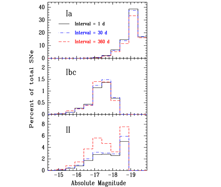
Figure 10: The observed LFs in a magnitude-limited sample. The solid line shows the results of an ideal magnitude-limited survey (with an observation interval of 1 d), while the dot-dashed and dashed lines show the results with longer observation intervals.

Figure 10 shows the histograms of the LFs of SNe in a magnitude-limited sample showing the percent of the total number of SNe for each bin (solid lines, with interval = 1 d), while Column 8 of Tables 3–5 lists the relative fraction of each SN assuming the total number of SNe is the same as in the volume-limited sample for each type. Compared to the volume-limited LFs, the magnitude-limited LFs clearly have an enhanced fraction of more luminous objects due to their larger survey volume. The average absolute magnitudes are $-19.00$ ($\sigma=0.46$) , $-17.29$ ($\sigma=0.62$), and $-17.70$ ($\sigma=0.85$) for SNe Ia, Ibc, and II, respectively, which are about 0.5, 1.2, and 1.6 mag brighter than those in a volume-limited sample. We also note that the scatter of the average absolute magnitude becomes smaller in a magnitude-limited sample, so the SNe appear to be more “standard” because of the redistribution of the SN fractions. In other words, a magnitude-limited search will be strongly biased in favour of luminous, unextinguished objects. One needs to be aware of this selection bias before generalizing a result derived from a magnitude-limited search. We note the SN Ibc absolute magnitude is now more in line with the average of the observed sample in Richardson et al. (2002), suggesting that a significant fraction of the observed SNe Ibc in their sample were discovered in magnitude-limited surveys.

4.2 The Observed Fractions of SNe

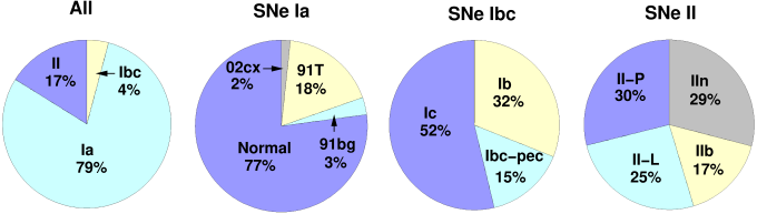
Figure 11: The observed fractions of the subclasses of SNe in an ideal magnitude-limited sample, illustrated as pie charts.

Because different subclasses of SNe have different absolute magnitudes, their observed fractions also change in a magnitude-limited survey, as shown in Figure 11 and listed in Table 7 (the column marked with “mag-1d”). The uncertainties of the fractions are derived from the Monte Carlo simulations discussed in §3.2. This is again for an ideal magnitude-limited survey in which the survey volume is constantly monitored. SNe Ia, the most luminous type of the three, now become the most abundant, accounting for 79% of the total. SNe II, the most abundant in a volume-limited sample, are only 17% of the total, while SNe Ibc are just 4%.

Among SNe Ia, normal SNe Ia are 77% of the total, SN 1991T-like objects are 18%, while SN 1991bg-like and SN 2002cx-like objects are 3% and 2%, respectively. The slow-evolving objects (SN 1991T-like objects and some normal SNe Ia) have enhanced numbers in a magnitude-limited survey because they are more luminous than the rest of the SNe Ia. The number of fast-evolving SN 1991bg-like objects, on the other hand, is depressed due to their subluminous nature. We also note that there may be hints that SN 1991bg-like objects constitute less than 3% of the total in some magnitude-limited surveys conducted at moderate and high redshifts, such as the Sloan Digital Sky Survey (SDSS; B. Dilday, 2009, private communication; Foley et al. 2009a) and the SN Legacy Survey (A. Howell, 2009, private communication), suggesting further discrimination against them at large look-back times. This, if confirmed, will constrain the progenitors of SN 1991bg-like objects to a tight range of old populations.

The fractions for the different subclasses of the CC SNe also change significantly, especially among SNe II. The fractions for SNe IIb and II-L are enhanced, while that for SNe II-P is depressed. It is worth noting that SNe II-P, the most abundant SN II component (70% of all) in a volume-limited survey, constitute only 30% of all in a magnitude-limited survey due to their subluminous nature.

4.3 The Effect of Observation Intervals

The previous two sections discuss the LFs and subclass fractions of SNe in an ideal magnitude-limited survey, one with the minimum observation interval (1 d). In practice, the observation intervals are significantly longer than 1 d in most magnitude-limited surveys, and we discuss their effect in this section.

We perform a Monte Carlo simulation similar to that employed by Li, Filippenko, & Riess (2001) to achieve this goal. The limiting magnitude of the survey is set to be 19, and the survey period is 10 yr. We use 10⁷ SNe in the simulation, and they are randomly but evenly distributed in a volume with the boundary set at a distance modulus $\mu$ = 40.0 mag. This large volume ensures that the survey is in the magnitude-limited regime even for the most luminous SNe in the LFs. Each SN is randomly selected from a LF that is constructed by combining the SN Ibc LF, the SN II LF, and the SN Ia LF within 80 Mpc scaled to $D=60$ Mpc (by a constant equal to the ratio of the total number of SNe in the two LFs), with a probability proportional to its number fraction. The SN is also given a random explosion date during the 10 yr period. The survey then goes through the series of dates of observations (according to the observation interval) and checks to see whether the SN is detected. In these simulations, a step function is used for the detection efficiency; the SN is marked as being detected when it is brighter than the survey limiting magnitude at any epoch of its light curve.

The effect of the observation interval on the LFs is shown in Figure 10. The shape of the LFs has subtle changes for all three SN types. The most significant change, however, is that more SNe II (with a higher percentage of total SNe) are discovered when the observation interval is longer. This is due to the fact that SNe II-P have a long plateau phase and their discovery rate is relatively enhanced with long observation intervals.

The subclass fractions with different observation intervals are shown in Figure 12 and listed in Table 7. The upper-left panel shows the overall SN Ia, Ibc, and II fractions. The SN Ibc fraction remains small, $\sim 4$% for all of the intervals. The SN Ia fraction decreases from 79% to 69%, while the SN II fraction increases from 17% to 27%, when the observation interval changes from 1 d to 360 d (or a single snapshot), respectively. Also shown in the panel is the curve of the “detection fraction,” which is the total number of SNe detected at a given observation interval divided by that with an observation interval of 1 d. The detection fraction remains high ($>94$%) when the observation interval is smaller than 10 d, and then declines dramatically with longer intervals. This is likely due to the fact that most SN light curves do not change much during the 10 d near maximum brightness. In a snapshot survey (i.e., with an interval of 360 d), only 8.6% of the SNe are detected.

The other panels show the subclass fractions with different observation intervals for SNe Ia, Ibc, and II, respectively. We note that when the observation interval is shorter than 10 d, all subclass fractions remain nearly unchanged. At longer intervals, the fractions of the SNe with relatively slow light curves are enhanced, e.g., SN 1991T-like objects among SNe Ia and SNe II-P among SNe II. In a snapshot survey, nearly 40% of the SNe II are SNe II-P, much higher than the fraction of 30% in an ideal magnitude-limited survey.

4.4 Comparisons to the Observed Magnitude-Limited Samples

To check whether our predicted subclass fractions of SNe in a magnitude-limited sample match observations, we compare our results to those of several actual magnitude-limited samples.

Although LOSS is a search with a targeted list of nearby galaxies, the random galaxies projected in the background of the LOSS target fields have a wide range of redshift, so the SNe discovered in them should only be limited by the depth of our images; they belong to a magnitude-limited sample. Gal-Yam et al. (2008) compiled a list of 32 such events discovered during the years 1999–2006. Here we update the list to include all of the SNe discovered during the years 2007–2008. We also revise the list of Gal-Yam et al. to exclude three objects (SNe 2002ct, 2003im, and 2004X; all occurred in targeted galaxies with relatively high redshift), and include six additional objects (SNe 2001ew, 2002je, 2002ka, 2004as, 2004eb, and 2005bu; all occurred in the background galaxies).

The full list has 47 SNe and is reported in Table 7. Only 1 object (SN 2001es) does not have a spectroscopic classification. For the rest of the SNe, 34 (74%) are SNe Ia, 4 (9%) are SNe Ibc, and 8 (17%) are SNe II. As the observation interval of our search is on average smaller than 10 d (Paper I), the observed fractions should be compared to those predicted by an ideal magnitude-limited search (79%, 4%, and 17% for SNe Ia, Ibc, and II, respectively), and they show excellent agreement. Comparison with the detailed subclasses is not possible because we do not have good light-curve coverage for these SNe, and the total number of CC SNe (12) is small.

The Palomar Transient Factory (PTF, Law et al. 2009) is a wide-field survey aimed at a systematic exploration of the optical transient sky, and is a classical magnitude-limited search for SNe. Two batches of SNe have been reported by Kasliwal et al. (2009) and Quimby et al. (2009). Among the 29 spectroscopically classified SNe (out of 31 total), 21 (72%) are SNe Ia, 1 (3%) is a SN Ibc, and 7 (24%) are SNe II. Considering the small total number of SNe involved, and the unknown observation interval, these fractions are in sufficiently good agreement with our predictions.

5 Discussion

In this section, we discuss the dependence of the volume-limited LFs on the environments and subclasses of SNe. We also consider possible applications of our LFs.

5.1 LFs in Galaxies of Different Sizes

As described in Paper I, the LOSS galaxy sample has an apparent deficit of low-luminosity galaxies when compared to a complete sample. It is thus important to study the correlation between the LFs and the galaxy sizes, and investigate whether the LFs we derived are biased because of this deficit.

Figure 13 shows the correlation of the LFs of SNe Ia with galaxy sizes. The top panel shows the LFs for the total SNe in the E–Sab (left) and Sb–Irr (right) galaxies, while the middle and bottom panels split the LFs into two host-galaxy size bins according to their $K$-band luminosities, with roughly equal numbers of SNe in each bin. Galaxy size does not play a significant role in the LFs of SNe Ia: K-S tests do not provide strong evidence for a significant difference in the two LFs for different galaxy sizes. We note that the bigger Sb–Irr galaxies host more SNe in the two most luminous bins and the bins at around $-17.5$ mag than the smaller galaxies, suggesting a possible more extreme LF in the bigger galaxies.

The total number of SNe in the SN Ibc LF sample is small (28.9). While we do not find any significant difference in the LFs for the galaxies with different sizes, the constraint is not strong due to small-number statistics.

Figure 14 shows the correlation of the LFs of SNe II with galaxy sizes. No significant difference is found for the early-type spirals, with the SNe in the two LFs coming from the same population at a $32.7^{+17.6}_{-15.1}$% probability. For the late-type spirals, this probability is $4.2^{+9.0}_{-2.6}$%, suggesting a rather significant difference. Even when the SNe fainter than $-15$ mag are not considered, the probability is still small ($4.5^{+11.2}_{-3.2}$%). The SNe II in the bigger late-type spirals are on average brighter than those in the smaller galaxies (the average is $16.28\pm 0.35$ [$\sigma=1.52$] and $-15.42\pm 0.25$ [$\sigma=1.12$], respectively). Inspection of the SNe in the two LFs suggests that the difference is likely caused by the different composition of subclasses. For the 18 SNe II in the smaller late-type spirals, there are 3 SNe IIb, 4 SNe IIn, and 11 SNe II-P, while for the 19 SNe II in the bigger late-type spirals, there are 2 SNe IIb, 3 SNe II-L, and 14 SNe II-P. Thus, it appears that SNe IIn might prefer smaller galaxies while SNe II-L prefer bigger galaxies (but keep in mind the small-number statistics). When only SNe II-P are considered, no significant difference is found in the two LFs.

In summary, we have not found a significant correlation between the LFs of SNe and their host-galaxy sizes, although some subclasses of SNe may have a preference to occur in certain galaxy sizes among some Hubble types. More discussion of this topic can be found in §5.4.

5.2 LFs in Galaxies of Different Inclinations

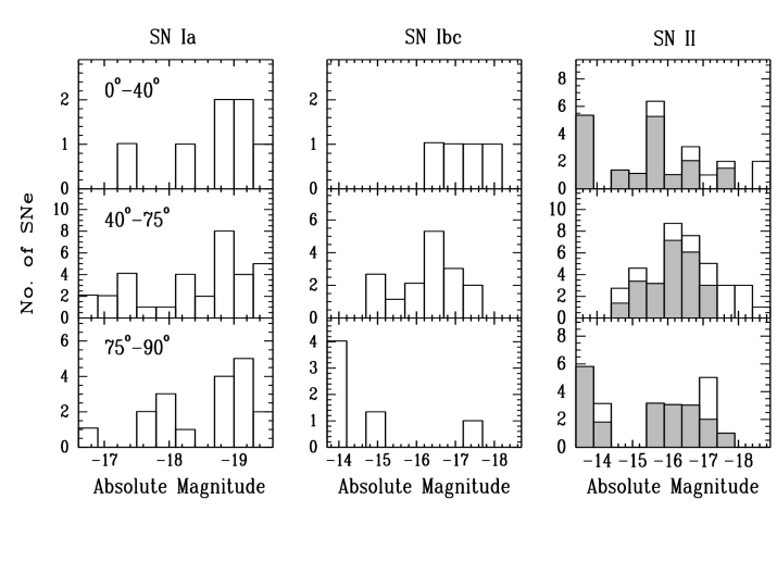
Figure 15: The LFs of SNe in host galaxies with different inclinations. For the SN II LFs, the shaded histogram is for the LF of the SNe II-P in the sample.

It is of interest to check the LFs of SNe in galaxies having different inclinations, and to investigate the effect of inclination on the amount of extinction the SNe experienced in their host galaxies. For this purpose, the LF SNe are split into three inclination bins ($0^{\circ}-40^{\circ}$ [hereafter, “face-on”], $40^{\circ}-75^{\circ}$ [hereafter, “inclined”], and $75^{\circ}-90^{\circ}$ [hereafter, “edge-on”]), and their LFs are plotted in Figure 15. Only the SNe occurring in spiral galaxies (Types 3 to 7) are considered because the inclination is not meaningful for an early elliptical or irregular galaxy, as discussed in Paper I. Because of the limitation of the total number of SNe in the LF sample, several LFs suffer from small-number statistics, especially SNe Ia and Ibc in the face-on bin, and SNe Ibc in the edge-on bin.

The LFs of SNe Ia do not show a significant difference in the three inclination bins, as reflected in the average absolute magnitudes in Table 6 and the K-S test results. The inclined and the edge-on bins both have a reasonable number of SNe (33.4 and 18.2, respectively). Moreover, because of the extraordinary luminosity of SNe Ia, our survey should have missed very few objects (even for SNe with moderate to high, but not extreme, extinction), as indicated by the small corrections to 100% completeness. Thus, perhaps surprisingly (given that many SNe Ia occur in young to intermediate-age populations; e.g., Maoz et al. 2011, and references therein), our data do not provide strong evidence for more extinction in more highly inclined galaxies for SNe Ia.

The LFs of SNe Ibc show a strong trend in the three inclination bins: the average absolute magnitude is the brightest in the face-on bin and the faintest in the edge-on bin. This is consistent with more extinction in more inclined galaxies. However, both the face-on and edge-on bins suffer from small-number statistics.

The LFs of SNe II have reasonable numbers of SNe in all three inclination bins. An unexpected result is that the LF for the objects with intermediate host-galaxy inclination ($40^{\circ}-75^{\circ}$) shows a significant difference from the LFs in the other two inclination bins, with an average absolute magnitude that is 0.7–0.9 mag brighter (Table 6). This difference becomes insignificant when only the objects brighter than $-15$ mag are considered. The LFs in the face-on and edge-on bins, on the other hand, show no significant difference. Thus, the LFs of SNe II do not provide evidence for more extinction in more highly inclined galaxies, in contrast with expectations.

We note that the LFs of SNe II in the different inclination bins could be affected by different subclass distributions. To investigate this, we plot the LFs of the most common subclass in Figure 15 (SNe II-P; shaded histogram). As can be seen, the SN II-P LFs exhibit a trend similar to that of the total SN II LFs.

Overall, our data do not provide evidence for more extinction in more highly inclined galaxies, a puzzling result. We emphasise, however, that because of small-number statistics and the deviation from Poisson statistics (due to the use of the corrected numbers of SNe), this result should be considered preliminary and needs to be checked with a significantly larger sample. For example, the lowest luminosity bin in the face-on SN II LF has a corrected number of SNe of 5.4, but it contains only two observed objects, SNe 1999br and 2002hh. When these two SNe are not considered, the LFs in the face-on and the $40^{\circ}-75^{\circ}$ bins do not show a significant difference and the LF in the edge-on bin is on average fainter by $\sim 1$ mag, consistent with a trend due to extinction.

5.3 LFs for Different SN Subclasses

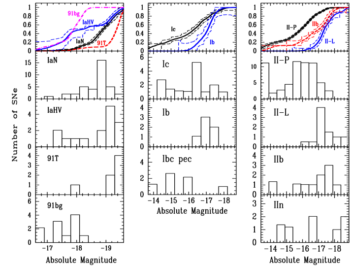
Figure 16: The LFs of SNe in different subclasses. The top panels show the cumulative fractions for selected SN subtypes. The dashed lines show the $1\sigma$ spread in the cumulative fractions considering only the uncertainties in the peak absolute magnitudes.

Since this is the first census of the subclasses for a complete sample of SNe, it is of interest to compare the LFs of different subclasses, as shown in Figure 16. The LFs of the different subclasses of SNe Ia show apparent differences. As expected, SN 1991bg-like objects are subluminous, while SN 1991T-like objects are overluminous. The two groups of normal SNe Ia with different expansion velocities exhibit a marginal 2–3$\sigma$ difference, as indicated by the cumulative fractions shown in the top panel. The LF of SNe IaHV is more skewed toward luminous objects, while it also has more objects at the faintest end. As discussed by Wang et al. (2009), SNe IaHV may have a different reddening law or colour evolution, and on average seem to suffer more extinction than SNe IaN. In fact, the two SNe in the faintest bin of the SN IaHV LF are SN 1999cl (Blondin et al. 2009) and SN 2006X (Wang et al. 2008), both highly reddened objects. Thus, SNe IaHV may be among the intrinsically brightest SNe Ia, though small-number statistics must be kept in mind.

SNe Ib appear to have a different LF (brighter with a smaller scatter) than SNe Ic (the averages are $-17.01\pm 0.17$ mag [$\sigma=0.41$] and $-16.04\pm 0.31$ mag [$\sigma=1.28$], respectively). However, this result is based on small-number statistics (as reflected by the error bars of the cumulative fractions shown in the top panel), and as discussed in §3.2, the classification of SNe Ibc into subclasses is still quite uncertain. More objects with definitive spectral classifications are needed to verify this result. The peculiar SNe Ibc are represented by only a small number of objects and exhibit a wide range of luminosities.

The different subclasses of SNe II have significant differences in their LFs. The least to most luminous subclasses are SNe II-P (with an average absolute magnitude of $-15.66\pm 0.16$ [$\sigma=1.23$]), SNe IIb ($-16.65\pm 0.40$ [$\sigma=1.30$]), SNe IIn ($-16.86\pm 0.59$ [$\sigma=1.61$]), and SNe II-L ($-17.44\pm 0.22$ [$\sigma=0.64$]). The LF of SNe II-P is different from that of the other three subclasses (even when the objects fainter than $-15$ mag are not considered), while there is no significant difference between SNe IIb and II-L. SNe IIn have a wide range of luminosities, including several of the most luminous objects.

To investigate whether the different subclasses of SNe have any preference in their host-galaxy Hubble types, we show the distribution in Figure 17. While the CC SNe display significant differences in their LFs, their host-galaxy Hubble-type distributions do not exhibit any significant differences. For SNe Ia, only SN 1991bg-like objects show a significant difference in their host-galaxy Hubble-type distribution: they have a strong preference to occur in elliptical and early-type spiral galaxies. SN 1991T-like objects, generally thought to have a strong preference to occur in spiral galaxies, are represented by only 5 objects in our LF SN sample, so their host-galaxy distribution is not well constrained. We also note that the host galaxy of SN 1998es, a SN 1991T-like object, may be misclassified as an early S0 galaxy. Van den Bergh, Li, & Filippenko (2002), for example, classified the galaxy as an early-type spiral galaxy (Sab in the DDO system).

5.4 The Host-Galaxy Properties of the LF SNe

Paper I discussed the host-galaxy properties of the full SN sample, in particular the Hubble-type distribution (its §4.2.3 and Figure 5). Here we examine the host-galaxy properties for the SNe in the LF sample.

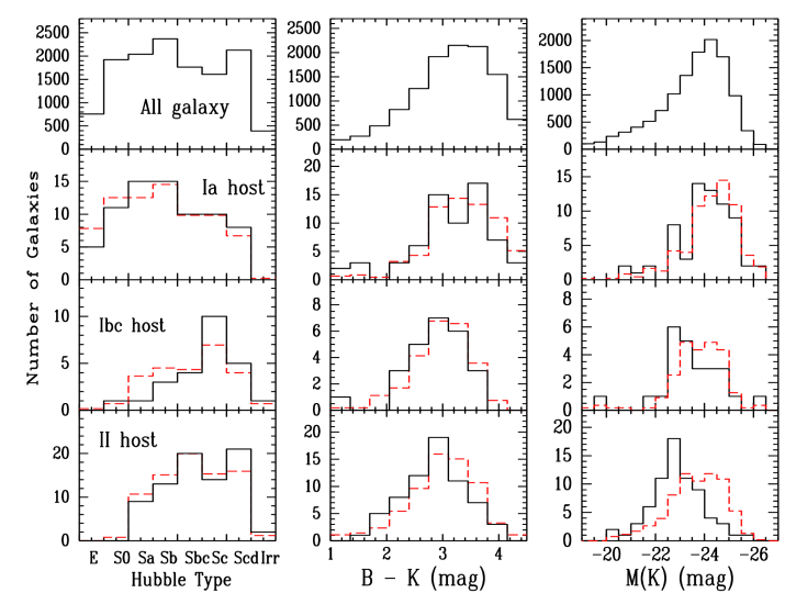
Figure 18: The SN host-galaxy properties. The left panels show the Hubble-type distribution, the middle panels the $B-K$ colour, and the right panels the $K$-band absolute magnitude, $M(K)$. From top to bottom, the statistics are shown for the “full-nosmall” galaxy sample, the SN Ia hosts, the SN Ibc hosts, and the SN II hosts. For the hosts of individual SN types, the solid lines are for the LF sample, while the dashed lines are for the “season-nosmall” SN sample scaled to the same number of SNe as in the LF sample.

Figure 18 illustrates the histograms for the Hubble-type distribution, the $B-K$ colour, and the absolute $K$-band luminosity $M(K)$. The top panels show the statistics for the “full-nosmall” galaxy sample, while the lower panels display the statistics for the hosts of SNe Ia, SNe Ibc, and SNe II, respectively. The histograms for the individual SN types are drawn with solid lines for the LF SNe, while the dashed lines are for the “season-nosmall” SN sample, scaled to the same number of SNe as in the LF sample.

We note that in general, the host galaxies of individual SN types display significant differences in their properties compared to the “full-nosmall” galaxy sample. This suggests that the different SN types have some degree of preference to occur in certain types of host galaxies. The SN Ia host galaxies are more skewed toward red $B-K$ colours and high $K$-band luminosities. The CC SNe, on the other hand, prefer galaxies with late Hubble types, blue $B-K$ colours, and low $K$ luminosities.

For a given type of SN, there are notable differences between the SNe in the season-nosmall (dashed lines) and LF (solid lines) samples. Overall, the host galaxies of the “season-nosmall” SN sample tend to be skewed toward earlier-type, redder, and more luminous galaxies. This is likely caused by the evolution of the galaxy properties over distance in our sample due to selection biases, as discussed in Paper I. The “season-nosmall” SN sample includes many SNe that occurred in the galaxies that are more distant than the cutoff distance for the LF SN sample, which, as discussed in §4.2.4 and Figure 4 of Paper I, have a higher fraction of bright, early-type galaxies than the more nearby galaxies.

The SN Ia hosts in general have properties that differ from those of the CC SN hosts. The SN Ibc and SN II hosts, on the other hand, have similar distributions for the Hubble types and $B-K$ colours, but different $M(K)$ distributions (with a 1.8% probability of coming from the same population). The host galaxies of SNe II are typically less luminous than those of SNe Ibc, with the average $M(K)=-22.92\pm 0.12$ mag ($\sigma=1.13$ mag) and $-23.42\pm 0.22$ mag ($\sigma=1.20$ mag), respectively. If SNe Ibc come from a similar population of massive stars (perhaps in binary systems) as those producing SNe II, their preference to occur in more luminous galaxies may indicate a metallicity effect (e.g., Tremonti et al. 2004) on the evolution of massive stars, such as by affecting the line-driven winds for the massive star that eventually explodes as the SN (Vink et al. 2001; Heger et al. 2003; Vink & de Koter 2005; Crowther 2007). Our suggestion that SNe Ibc occur in galaxies of higher luminosity or metallicity than SNe II is consistent with the findings of Prantzos & Boissier (2003), Prieto, Stanek, & Beacom (2008), and Boissier & Prantzos (2009).

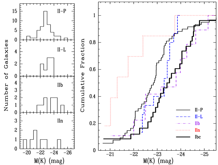
Figure 19: The host-galaxy $M(K)$ distribution for the different SN subclasses (left panels) and the cumulative fractions (right panel) for the LF SN sample.

We also investigate whether the different SN subclasses have different host-galaxy $M(K)$ distributions. For SNe Ia, the only significant difference is found between the host galaxies of the SNe IaN and SNe Ia-91bg subclasses, with the hosts of SNe Ia-91bg being more luminous on average due to the dominance of earlier Hubble types. The results for the CC SN subclasses are shown in Figure 19. The left panels display the histograms of the $M(K)$ distributions while the right panel shows the cumulative fractions. Several subclasses still suffer from small-number statistics; nevertheless, we find the following trends with varying significance.

1. No significant difference is found between the host galaxies of SNe II-P and II-L, though the total number of SNe II-L is small (7.5).

2. No significant difference is found between the host galaxies of SNe Ib and Ic, with a 28.0% probability that they come from the same population. The average $M(K)$ of the hosts of SNe Ib ($-24.20\pm 0.46$ mag [$\sigma=1.15$ mag]) appears to be marginally more luminous than the hosts of SNe Ic ($-23.22\pm 0.34$ mag [$\sigma=1.35$ mag]). In the cumulative fraction plot, the two subclasses are combined.

3. The host galaxies of SNe IIb are more luminous than those of SNe II-P, with a 6.9% probability that they come from the same population. The average $M(K)$ values are $-23.54\pm 0.42$ mag ($\sigma=1.28$ mag) and $-22.84\pm 0.14$ mag ($\sigma=1.11$ mag), respectively. Furthermore, there is a relatively high probability (68.5%) that the host galaxies of SNe IIb and Ibc come from the same population, as can be seen by the similar cumulative fraction curves in the right-hand panel of Figure 19.

4. The host galaxies of SNe IIn are less luminous than those of SNe II-P, with a 10.3% probability that they come from the same population. The average $M(K)$ value is $-22.08\pm 0.54$ mag ($\sigma=1.40$ mag) for the SN IIn host galaxies.

As discussed in Paper I, the LOSS galaxy sample involves several selection biases, and is not complete at the low-luminosity end. Nevertheless, since all of the SNe were discovered in the same set of galaxies and thus suffer from the same selection biases, the above trends still reveal the general preference for the different subclasses of SNe in terms of host-galaxy $K$-band luminosities.

Recently, Arcavi et al. (2010) reported on the statistics of 70 CC SNe found by PTF and suggested that there might be an excess of SNe IIb and Ib in dwarf galaxies, which differs from our finding that the host galaxies of both subclasses prefer more luminous galaxies. As PTF is conducting an untargeted, magnitude-limited survey and monitors numerous dwarf galaxies, the study by Arcavi et al. (2010) is complementary to ours. The differences in the results might be caused by the relatively small numbers of objects in both studies, although Poisson statistics have nominally been taken into account. Perhaps the discrepancy is related to the dissimilar analysis methods; we study the differences in the $M(K)$ distributions of the SN host galaxies, while Arcavi et al. (2010) divided the galaxies into two categories (giant/dwarf) and analysed the fractions of the different SN subclasses. Further studies are needed to verify the apparent discrepancy between the two results.

5.5 Possible Limitations and Caveats for Our LFs

One limiting factor of our LFs is the total number of SNe in the sample. Although much effort has been made to analyse the data for the 175 SNe in our LF sample, many analyses still face small-number statistics, such as the LFs for the different subclasses of SNe. As shown in Figure 4, the cutoff distance for the SN Ia LF sample can be increased to 120 Mpc to include more SNe without introducing large corrections due to incompleteness. For the CC SNe, the inclusion of the data in the years 2007–2008 will help increase the sample in the LF. We are in the process of reducing more data to continue working along these directions, and the results will be published in a future paper.

Another limiting factor of our LFs is that they are only available for the $R$ band. For SNe Ia, a significant fraction of the LF SNe have been followed in $BVRI$, and the multi-colour LFs will be presented in a future paper. For SNe Ibc and SNe II, only a small fraction of the LF SNe have filtered follow-up photometry, so determining their multi-colour LFs is not possible at this time. It will require considerable effort to obtain filtered photometry for all of the relatively low-luminosity CC SNe in either a volume-limited or magnitude-limited survey to construct the LFs in different passbands.

One concern is that the LFs we derived only apply to our galaxy sample with its specific Hubble type, colour, and luminosity distributions. As discussed in detail in Paper I, however, the galaxy sample within the cutoff distance for the LFs is probably representative of galaxies with moderate and large sizes, and only has an apparent deficit for small galaxies. This deficit may cause our LFs to be biased against those SNe having a preference to occur in small galaxies. In our study, we only find a possible preference for SNe IIn to occur in small, late-type spiral galaxies.

We excluded the SNe that occurred in small (major axis $<1\arcmin$), early-type galaxies because of uncertainties in the detection efficiencies. One concern is whether this exclusion introduces an observational bias. No SNe Ibc or II are excluded because CC SNe in early-type galaxies are rare (§4.2.3 in Paper I). For SNe Ia, only two objects (SNe 2000dk [IaN] and 2006H [Ia-91bg]) are excluded. Considering that the total SN Ia LF has 74 SNe Ia, the inclusion of the two additional SNe will have negligible effect on the overall properties of the SN Ia LF.

One important question is whether there is a sizable fraction of highly reddened SNe that are missed in our search. Some SNe certainly experience a large amount of extinction; for example, the SN Ia 2002cv (Di Paola et al. 2002; Elias-Rosa et al. 2008) has $A_{V}\approx 9$ mag, while the SN II-P 2002hh suffered $A_{V}\approx 5$ mag (Pozzo et al. 2006). Searches done at near-infrared and radio wavelengths also suggest that the vast majority of SNe in massive starburst galaxies, such as luminous infrared galaxies (LIRGs) and ultraluminous infrared galaxies (ULIRGs), are missed by the optical searches due to dust obscuration (e.g., Mannucci et al. 2003).

We argue, however, that our LFs are not significantly affected by host-galaxy extinction for the following reasons. First, LIRGs/ULIRGs constitute only a very small fraction of the galaxy population. Second, for a non-starburst galaxy, although the theoretical studies of Hatano et al. (1998) and Riello & Patat (2005) suggest that SNe should experience more extinction in more highly inclined galaxies, our investigation of the LFs in different inclination bins (§5.2) does not provide strong supporting evidence. Third, statistics provided by the observed SN sample (Jha et al. 2006a; Hicken et al. 2009) indicate that the majority of the observed SNe Ia do not suffer significant amounts of extinction. Finally, our own LFs provide additional evidence for the scarcity of highly reddened events: only a few of the 175 SNe in the LF sample suffer a large amount of extinction (SNe 2001ci, 2002hh, 2003bk, 2003cg, and 2005bb). For our typical search limiting magnitude of 19, we can detect SNe brighter than $-12.5$, $-13.4$, and $-14.9$ mag within 20, 30, and 60 Mpc, respectively. These are several magnitudes fainter than the average SNe in the LF, so we should have discovered many more moderately reddened objects ($A_{V}$ of a few mag) near our detection limit if highly reddened SNe were quite common. We conclude that our LFs are not significantly affected by the missing SNe due to high extinction in the targeted sample galaxies.

5.6 Possible Applications of our LFs

Our LF data (tables and template light curves) are made available to interested parties electronically. These LFs have the following potential applications.

1. The LFs can be used to calculate the control times for the different types of SNe in a SN search, which is a critical step in deriving the SN rates. This is the main motivation for our study. Paper III will discuss the details of how the LFs are used to calculate the control times in our SN search. Any other SN searches conducted without filters or using a passband that is similar to $R$ could use our LFs to help with the control-time and/or survey-completeness calculation. A major advantage of using our LFs to calculate the control times is that they are “pseudo-observed” and account for the poorly known host-galaxy extinction.

2. The LFs can be used to simulate the expected SN subclass and brightness distribution in a SN search (with known cadence and depth), to help the coordination of follow-up efforts. For this purpose, the SN rates derived in Paper III are needed as well.

3. The LFs, the light-curve distributions, and the observed subclass fractions can be used as priors in a photometry-based classification scheme, as in Poznanski et al. (2002) and Poznanski, Maoz, & Gal-Yam (2007).

4. The LFs can be used to constrain the possible progenitor systems and their evolutionary paths for the different types of SNe. Viable models should be able to explain both the luminosity distribution and the various subclass fractions (e.g., Smith et al. 2011a).

6 Conclusions

Historically, SN rate calculations have been plagued by two issues: the intrinsic luminosity distribution of SNe and the host-galaxy extinction toward SNe. In other words, the calculations were limited by our knowledge of the observed luminosity functions of SNe. In this Paper II of a series aimed to derive a precise nearby SN rate from the Lick Observatory SN Search, a volume-limited SN sample is constructed for the first time, and the observed luminosity functions of SNe are derived.

We first select a volume-limited sample of 175 SNe (with a cutoff distance of 80 Mpc for SNe Ia, and 60 Mpc for SNe Ibc and SNe II), and then collect photometry for every object. Families of light curves for each SN type are constructed from the literature and/or our own photometry database, and are used to fit the light curves of the SNe, to generate peak absolute magnitude and light-curve shape distributions. We further study the completeness of each SN in the LF, and correct them to 100% completeness within the considered volume.

The volume-limited LFs of SNe indicate that a Gaussian scatter around an average luminosity is generally not a good representation of the data. There are also significant differences for the LFs in different host-galaxy Hubble types. For SNe Ia, the SNe in E–Sab galaxies are generally fainter than those in Sb–Irr galaxies due to the prominence of subluminous SN 1991bg-like objects in the former galaxies. For SNe Ibc, the objects in early-type spirals are, on average, slightly fainter than those in late-type spirals. For SNe II, the objects in early-type spirals are, on average, brighter than those in late-type spirals. These observed trends have significant implications for their possible progenitor systems and evolutionary paths.

We also have detailed subclass information for all SNe in the LF sample. While spectral series are adequate to classify SNe Ia and Ibc into different subclasses, detailed light-curve information is necessary to discriminate the different subclasses of SNe II, especially SNe II-P, II-L, and IIb. In a volume-limited sample, SNe II are the most abundant type (57% of all), while SNe Ia and Ibc constitute 24% and 19%, respectively. For SNe Ia, normal objects are 70% of all, SN 1991bg-like objects are 18%, and the rest are SN 1991T-like and SN 2002cx-like objects (12%). The normal SNe Ia are further split into objects with normal (50%) and high (20%) expansion velocities. SNe Ic are the most abundant SNe Ibc (54% of all), while SNe II-P are the most abundant SNe II (70% of all). Among SNe II, there are significant fractions of SNe II-L, IIb, and IIn (10%, 12%, and 9%, respectively).

We further derive the observed LFs and SN subclass fractions for an ideal magnitude-limited search (i.e., with a short observation interval) by scaling the SNe with their survey volume. Compared to the volume-limited LFs, the magnitude-limited LFs have an enhanced fraction of luminous objects, as well as reduced scatter in the average luminosity. The observed fractions of SNe have also dramatically changed. SNe Ia are the most numerous SNe (79%) of the three types, while the fractions of the core-collapse SNe shrink to 17% and 4% for SNe II and Ibc, respectively. Within SNe Ia, normal SNe Ia are 77% of all, and SN 1991T-like objects are boosted to 18%. SNe Ibc become as abundant as SNe Ic among the SNe Ibc. The fractions of SNe II-L, IIb, and IIn are enhanced due to their higher luminosities than those of SNe II-P. We compare our predicted subclass fractions to two observed magnitude-limited samples, one in the random background galaxies in our own search, and the other from PTF, and find good agreement.

We also investigate the effect of the observation interval in a magnitude-limited search on the observed LFs and SN fractions. Searches done with an observation interval smaller than 10 d have similar LFs and SN fractions, and discover a high fraction of the SNe in an ideal magnitude-limited search. When the observation interval is long, the fractions for the SNe with relatively slow light curves are enhanced. In a search with a very long interval (or a single snapshot), only $\sim 9$% of the SNe in an ideal magnitude-limited search are discovered, and SNe II-P become the dominant subclass (40% of the total) among SNe II.

We discuss how the LFs we derived change with different environments and subclasses of SNe. We have not found a persistent correlation between the LFs of SNe and their host-galaxy sizes, although some subclasses of SNe seem to have a preference to occur in certain galaxy sizes in some Hubble types (e.g., SNe IIn prefer small, late-spiral galaxies). Surprisingly, the LFs in galaxies of different inclination do not provide strong evidence in support of greater extinction toward SNe in more highly inclined galaxies. The different subclasses of SNe display significant differences in their LFs. For SNe Ia, the SN 1991bg-like objects are subluminous, while the SN 1991T-like objects are overluminous. The normal SNe Ia with high expansion velocities display a more extreme LF than the normal SNe Ia having normal expansion velocities, suggesting that they may belong to two distinct groups. SNe Ib are, on average, more luminous and have a smaller scatter than SNe Ic, but this result should be reexamined in a larger sample with more definitive spectral identifications than our current sample. The least to most luminous SNe II are II-P, IIb, IIn, and II-L. Despite the significant difference in the LFs, the different subclasses of core-collapse SNe show similar host-galaxy Hubble-type distributions. For SNe Ia, SN 1991bg-like objects prefer to occur in elliptical and early-type spiral galaxies. We note that some of these results have been found in previous work (e.g., Della Valle & Livio 1994; Hamuy et al. 1996; Howell 2001; Jha et al. 2006a).

We also compare the host-galaxy properties of the LF SNe, and find a significant difference in the galaxy luminosity distributions for SNe II and Ibc. SNe Ibc prefer more massive galaxies than SNe II, suggesting an influence of metallicity on the mass-loss history in their evolution. We also find that SNe IIb prefer more massive galaxies than SNe II-P, while SNe IIn prefer less massive galaxies.

We discuss possible limitations of our LFs; small-number statistics are the primary one. Caution should be used when applying our LFs to low-luminosity galaxies, but our LFs do not appear to be seriously affected by SNe missing due to large extinction.

Our LFs can be used to help with SN rate determinations for any searches using a passband similar to the $R$ band. Other applications of the LFs are to coordinate follow-up efforts in large surveys, help photometry-based classification methods, and constrain viable models for the SNe.

Figure 12: The observed subclass fractions in a magnitude-limited sample as a function of observation interval. Also shown in the upper-left panel is the “detection fraction” curve. See text for details.

Figure 13: The luminosity functions of SNe Ia in galaxies of different luminosities. The top panels show the LFs in the total sample, while the bottom two panels split the LF into two bins according to the $K$-band luminosities of their host galaxies.

Figure 14: Same as Figure 12 but for the LFs of SNe II.

Figure 17: The Hubble-type distribution of the different SN subclasses in the LF sample.

Table 1: Host galaxies of supernovae in the luminosity function sample.

SN	Type	Host Galaxy	$h$	Dist (Mpc)	$B_{0}$ (mag)	$B_{0}$(err)	$K$ (mag)	$K$(err)
1998dm	IaN	UGCA-017	6	25.8	12.128	0.683	10.442	0.055
1999cp	IaN	NGC-5468	7	39.4	12.767	0.208	10.396	0.059
1999ej	IaN	NGC-0495	2	57.8	13.237	0.391	9.965	0.031
1999ek	IaN	UGC-03329	5	72.0	11.960	0.500	9.780	0.032
1999gd	IaN	NGC-2623	3	77.0	13.163	0.146	10.427	0.027
2000dm	IaN	UGC-11198	3	64.2	13.500	0.407	10.532	0.034
2000dr	IaN	IC-1610	2	75.6	13.685	0.359	9.844	0.038
2001L	IaN	MCG-01-30-011	4	62.5	13.058	0.419	9.916	0.039
2001dn	IaN	NGC-0662	5	79.3	14.081	0.148	10.797	0.045
2001ep	IaN	NGC-1699	4	52.0	—	—	10.629	0.050
2001fh	IaN	Anon.-Gal.	7	57.8	11.174	0.153	8.531	0.029
2002cr	IaN	NGC-5468	7	39.4	12.767	0.208	10.396	0.059
2002do	IaN	MCG-+07-41-001	1	68.4	13.262	0.116	9.076	0.024
2002fk	IaN	NGC-1309	5	27.2	11.730	0.106	9.102	0.029
2002ha	IaN	NGC-6962	3	58.5	12.351	0.079	8.786	0.029
2002hw	IaN	UGC-00052	6	72.3	14.139	0.321	10.405	0.060
2002jg	IaN	NGC-7253B	6	63.8	13.200	0.893	99.999	0.000
2003F	IaN	UGC-03261	7	70.9	13.620	0.366	10.635	0.074
2003cg	IaN	NGC-3169	3	16.9	10.897	0.086	7.283	0.021
2003du	IaN	UGC-09391	7	30.1	14.652	0.080	—	—
2003gt	IaN	NGC-6930	3	63.8	12.683	0.200	99.999	0.000
2003kf	IaN	MCG-02-16-002	4	28.6	12.576	0.500	10.935	0.054
2004ab	IaN	NGC-5054	5	23.4	10.875	0.130	—	—
2004bd	IaN	NGC-3786	3	39.2	13.027	0.172	9.338	0.025
2004bl	IaN	CGCG-013-112	7	71.5	13.700	0.381	12.684	0.153
2005W	IaN	NGC-0691	5	37.2	11.687	0.202	8.822	0.038
2005am	IaN	NGC-2811	3	30.7	11.596	0.108	7.976	0.015
2005as	IaN	NGC-3450	4	53.7	12.314	0.204	8.501	0.048
2005bc	IaN	NGC-5698	4	53.5	13.208	0.307	10.287	0.049
2005bo	IaN	NGC-4708	3	56.2	13.488	0.290	10.140	0.053
2005cf	IaN	MCG–01-39-003	2	27.1	14.293	0.512	11.293	0.073
2005de	IaN	UGC-11097	4	65.6	13.276	0.410	10.434	0.040
2005el	IaN	NGC-1819	2	60.5	13.110	0.346	9.227	0.031
2005kc	IaN	NGC-7311	3	62.6	12.405	0.523	8.937	0.015
2006ax	IaN	NGC-3663	5	68.3	12.650	0.312	9.894	0.068
2006dy	IaN	NGC-5587	2	33.3	13.277	0.320	9.684	0.029
2006lf	IaN	UGC-03108	4	56.1	10.898	0.500	9.533	0.033
1998dh	IaHV	NGC-7541	5	37.0	11.386	0.087	8.351	0.007
1998dk	IaHV	UGC-00139	6	53.8	13.613	0.330	11.044	0.069
1998ef	IaHV	UGC-00646	4	74.2	13.841	0.327	10.428	0.038
1999cl	IaHV	MESSIER-088	4	32.6	9.563	0.129	6.267	0.017
1999dk	IaHV	UGC-01087	6	61.7	14.483	0.365	11.096	0.082
2001E	IaHV	NGC-3905	6	78.4	12.963	0.148	9.884	0.068
2001en	IaHV	NGC-0523	5	66.8	12.333	0.066	9.714	0.022
2002bo	IaHV	NGC-3190	3	19.1	11.397	0.226	99.999	0.000
2002dj	IaHV	NGC-5018	1	37.8	11.220	0.193	7.734	0.014
2002er	IaHV	UGC-10743	3	36.9	13.405	0.324	10.375	0.037
2004ca	IaHV	UGC-11799	6	76.1	13.141	0.500	10.300	0.066
2005A	IaHV	NGC-0958	6	77.5	11.857	0.049	8.800	0.020
2006X	IaHV	MESSIER-100	5	23.0	9.840	0.154	—	—
2006ef	IaHV	NGC-0809	2	72.1	14.406	0.421	10.597	0.035
2006le	IaHV	UGC-03218	4	74.4	12.321	0.560	9.208	0.024
1998de	Ia-91bg	NGC-0252	2	69.2	12.900	0.410	9.044	0.025
1999by	Ia-91bg	NGC-2841	4	11.4	9.537	0.116	6.062	0.019
1999da	Ia-91bg	NGC-6411	1	54.3	12.512	0.115	9.126	0.023
2002cf	Ia-91bg	NGC-4786	1	63.4	12.492	0.090	8.717	0.027
2002dk	Ia-91bg	NGC-6616	3	78.6	13.826	0.382	9.397	0.025
2002fb	Ia-91bg	NGC-0759	1	65.3	13.387	0.079	9.139	0.019

Table 1: continued …

SN	Type	Host	$h$	Dist	$B_{0}$ (mag)	$B_{0}$(err)	$K$ (mag)	$K$(err)
2002jm	Ia-91bg	IC-0603	3	73.5	14.334	0.409	10.431	0.052
2003Y	Ia-91bg	IC-0522	2	72.4	13.499	0.317	9.973	0.025
2005ke	Ia-91bg	NGC-1371	3	17.4	11.296	0.099	7.630	0.039
2005mz	Ia-91bg	NGC-1275	2	73.9	11.819	0.126	8.126	0.038
2006ke	Ia-91bg	UGC-03365	3	73.7	13.458	0.317	9.990	0.056
1998es	Ia-91T	NGC-0632	2	43.0	13.481	0.446	10.096	0.028
1999aa	Ia-91T	NGC-2595	6	60.1	12.672	0.200	9.661	0.046
1999ac	Ia-91T	NGC-6063	7	40.7	13.354	0.345	10.550	0.078
1999dq	Ia-91T	NGC-0976	6	59.4	12.679	0.059	9.114	0.021
2001V	Ia-91T	NGC-3987	4	63.5	12.989	0.182	9.046	0.017
2004bv	Ia-91T	NGC-6907	5	42.6	11.470	0.056	8.370	0.020
2006cm	Ia-91T	UGC-11723	4	67.5	13.702	0.341	9.988	0.028
1999bh	Ia-02cx	NGC-3435	4	74.0	13.525	0.410	10.726	0.046
2002es	Ia-02cx	UGC-02708	2	75.6	14.450	0.489	—	—
2005cc	Ia-02cx	NGC-5383	4	33.4	12.006	0.168	8.536	0.038
2005hk	Ia-02cx	UGC-00272	7	52.9	14.288	0.321	12.983	0.201
1998dt	Ib	NGC-0945	6	59.8	12.568	0.074	9.361	0.043
1999dn	Ib	NGC-7714	4	38.3	12.530	0.141	9.762	0.027
2001is	Ib	NGC-1961	6	57.1	10.971	0.089	7.730	0.035
2004dk	Ib	NGC-6118	7	22.5	11.060	0.077	8.703	0.019
2004gq	Ib	NGC-1832	5	24.4	10.658	0.516	8.388	0.025
2006F	Ib	NGC-0935	7	57.6	12.546	0.410	9.322	0.039
1999bu	Ic	NGC-3786	3	39.2	13.027	0.172	9.338	0.025
2000C	Ic	NGC-2415	8	53.5	12.329	0.235	9.776	0.020
2001M	Ic	NGC-3240	4	46.6	13.481	0.186	10.588	0.052
2001ci	Ic	NGC-3079	6	18.4	9.970	0.253	99.999	0.000
2002J	Ic	NGC-3464	6	49.7	12.490	0.076	9.464	0.046
2002jj	Ic	IC-0340	6	55.1	14.260	0.406	10.866	0.071
2002jz	Ic	UGC-02984	7	20.9	13.150	0.500	12.142	0.110
2003aa	Ic	NGC-3367	6	42.4	11.845	0.031	8.755	0.028
2004C	Ic	NGC-3683	6	26.6	12.238	0.385	8.666	0.022
2004cc	Ic	NGC-4568	5	32.0	10.959	0.100	7.516	0.026
2005az	Ic	NGC-4961	7	37.0	13.714	0.057	10.845	0.052
2005lr	Ic	ESO-492-G002	4	32.9	11.630	0.200	9.224	0.032
2006eg	Ic	CGCG-462-023	5	55.0	14.175	0.325	11.977	0.089
2002ap	Ic-pec	MESSIER-074	6	9.4	9.345	0.259	6.845	0.054
2003H	Ibc-pec	NGC-2207	5	35.2	11.328	0.303	8.190	0.037
2003dr	Ibc-pec	NGC-5714	6	34.1	12.691	0.327	9.968	0.033
2003id	Ic-pec	NGC-0895	7	30.1	11.875	0.104	9.405	0.051
2004bm	Ibc-pec/IIb	NGC-3437	6	18.9	11.673	0.421	8.878	0.015
2005E	Ibc-pec	NGC-1032	2	36.5	12.134	0.097	8.379	0.018
1999D	II-P	IC-0694	7	44.3	12.454	1.593	8.422	0.024
1999an	II-P	NGC-4019	4	22.0	13.107	0.634	11.334	0.056
1999bg	II-P	IC-0758	7	21.1	13.456	0.303	—	—
1999br	II-P	NGC-4900	6	13.9	11.762	0.093	8.638	0.038
1999em	II-P	NGC-1637	6	8.4	11.267	0.154	7.974	0.045
1999gi	II-P	NGC-3184	7	10.5	10.312	0.155	7.225	0.067
2000L	II-P	UGC-05520	7	48.8	13.783	0.273	11.686	0.078
2000cb	II-P	IC-1158	6	27.6	12.819	0.111	10.238	0.076
2000el	II-P	NGC-7290	5	41.1	13.015	0.037	10.739	0.051
2000ex	II-P	ESO-419-G003	6	53.4	13.245	0.321	10.945	0.072
2001J	II-P	UGC-04729	7	54.0	14.485	0.392	12.164	0.113
2001K	II-P	IC-0677	5	45.4	12.932	0.363	10.712	0.040
2001bq	II-P/II-L	NGC-5534	3	36.4	12.858	0.143	9.629	0.032
2001cm	II-P	NGC-5965	4	50.6	11.520	0.101	8.608	0.031
2001dc	II-P	NGC-5777	5	33.1	12.741	0.328	9.314	0.016
2001fz	II-P	NGC-2280	7	23.6	9.976	0.366	8.255	0.031
2002bx	II-P	IC-2461	5	32.9	13.502	0.420	10.052	0.020
2002ca	II-P	UGC-08521	3	45.7	13.965	0.324	10.352	0.050
2002ce	II-P	NGC-2604	7	29.8	13.497	0.427	11.044	0.060
2002dq	II-P	NGC-7051	3	34.5	12.963	0.375	9.467	0.025
2002ds	II-P	UGCA-402	7	30.7	11.736	0.243	9.117	0.021

Table 1: continued …

SN	Type	Host	$h$	Dist	$B_{0}$ (mag)	$B_{0}$(err)	$K$ (mag)	$K$(err)
2002gd	II-P	NGC-7537	5	36.9	12.678	0.059	10.213	0.027
2002gw	II-P	NGC-0922	7	39.9	12.165	0.088	10.023	0.068
2002hh	II-P	NGC-6946	7	4.4	8.237	0.217	5.369	0.034
2003E	II-P	ESO-485-G004	5	57.7	14.329	0.270	99.999	0.000
2003Z	II-P	NGC-2742	6	20.8	11.385	0.079	8.808	0.014
2003ao	II-P	NGC-2993	3	30.4	12.747	0.055	10.131	0.041
2003bk	II-P	NGC-4316	5	18.2	12.491	0.090	9.246	0.027
2003br	II-P	ESO-447-G023	7	50.7	13.088	0.212	10.391	0.051
2003bw	II-P	IC-1077	5	46.5	13.064	0.197	9.560	0.032
2003ef	II-P	NGC-4708	3	56.2	13.488	0.290	10.140	0.053
2003hg	II-P	NGC-7771	3	59.9	12.296	0.168	8.348	0.017
2003hl	II-P	NGC-0772	4	33.9	10.000	0.539	—	—
2003iq	II-P	NGC-0772	4	33.9	10.000	0.539	—	—
2003ld	II-P	UGC-00148	5	57.6	15.267	2.517	10.531	0.040
2004aq	II-P	NGC-4012	4	58.2	13.416	0.322	10.430	0.050
2004ci	II-P	NGC-5980	5	58.2	12.372	0.560	9.441	0.024
2004dd	II-P	NGC-0124	6	54.8	13.264	0.357	10.755	0.068
2004er	II-P	UGCA-036	6	59.3	13.585	0.384	10.734	0.081
2004et	II-P	NGC-6946	7	4.4	8.237	0.217	5.369	0.034
2004fc	II-P	NGC-0701	6	23.7	12.174	0.069	9.170	0.028
2004fx	II-P	MCG-02-14-003	6	34.8	99.999	99.999	10.413	0.042
2005ad	II-P	NGC-0941	6	20.8	12.625	0.090	10.694	0.080
2005ay	II-P	NGC-3938	6	13.9	10.802	0.033	7.809	0.048
2005bb	II-P	UGC-08067	4	39.3	13.621	0.678	10.420	0.061
2005ci	II-P	NGC-5682	4	34.7	14.040	0.163	12.250	0.059
2005io	II-P	UGC-03361	7	47.5	14.363	0.500	11.894	0.079
2005mg	II-P	UGC-00155	4	54.5	13.481	0.410	9.764	0.022
2006be	II-P	IC-4582	5	32.1	13.749	0.410	10.574	0.032
2006bp	II-P	NGC-3953	5	17.6	9.881	0.292	7.047	0.026
2006ca	II-P	UGC-11214	7	38.2	—	—	10.938	0.089
2006qr	II-P	MCG–02-22-023	5	58.0	13.781	0.500	10.962	0.057
1999go	II-L	NGC-1376	7	55.5	12.640	0.221	9.804	0.061
2000dc	II-L	ESO-527-G019	4	41.8	13.241	0.392	10.713	0.042
2001do	II-L	UGC-11459	7	46.0	12.862	0.332	9.775	0.046
2001hf	II-L	ESO-564-G015	5	59.6	12.934	0.200	99.999	0.000
2002an	II-L	NGC-2575	7	53.9	13.350	0.250	10.226	0.068
2005J	II-L	NGC-4012	4	58.2	13.416	0.322	10.430	0.050
2005an	II-L	ESO-506-G011	4	43.7	14.797	0.179	10.885	0.049
1999cd	IIb	NGC-3646	5	59.6	11.112	0.153	8.484	0.025
2000H	IIb	IC-0454	3	53.8	—	—	9.387	0.023
2001Q	IIb	UGC-06429	6	54.6	13.655	0.090	11.212	0.084
2003ed	IIb	NGC-5303	6	22.3	12.279	0.410	10.227	0.026
2004be	IIb	ESO-499-G034	7	29.3	14.650	0.200	—	—
2005H	IIb	NGC-0838	8	51.2	13.370	0.117	9.743	0.023
2005U	IIb	NGC-3690	7	46.3	13.142	3.595	—	—
2006T	IIb	NGC-3054	5	31.2	11.668	0.145	8.343	0.029
2000N	IIb/II-L	MCG–02-34-054	5	54.4	12.866	0.390	9.909	0.058
2004al	IIb/II-L	ESO-565-G025	4	58.1	14.280	0.297	11.319	0.061
1999el	IIn	NGC-6951	5	23.3	10.022	0.214	7.220	0.025
2000eo	IIn	MCG–02-09-003	3	41.2	13.318	0.366	11.046	0.075
2002bu	IIn	NGC-4242	7	10.1	11.260	0.185	—	—
2003G	IIn	IC-0208	5	47.7	14.291	0.318	10.679	0.081
2003dv	IIn	UGC-09638	8	34.9	15.779	1.055	—	—
2005aq	IIn	NGC-1599	6	53.4	13.870	0.030	12.182	0.115
2006bv	IIn	UGC-07848	7	37.9	13.700	0.310	11.768	0.064
1999bw	IIni	NGC-3198	6	11.7	9.947	0.202	7.779	0.042
2000ch	IIni	NGC-3432	7	10.7	10.583	0.120	9.061	0.050
2001ac	IIni	NGC-3504	3	22.9	11.434	0.133	8.273	0.014
2002kg	IIni	NGC-2403	7	5.1	8.114	0.098	6.191	0.039
2003gm	IIni	NGC-5334	6	19.6	12.430	0.729	9.935	0.047

Table 2: Average light curves of the supernovae (the numbers are magnitudes below peak brightness) ^a

t(day)	Ia.01	Ia.11	Ia.21	Ibc.fast	Ibc.ave	Ibc.slow	II-P	II-L	IIb	IIn.fast	IIn.ave	IIn.slow
-30.0	57.530	44.540	31.550	10.488	9.580	4.445	—	—	—	2.961	—	—
-29.0	54.660	42.160	29.660	10.065	8.974	4.134	—	—	—	2.827	—	—
-28.0	51.800	39.790	27.780	9.642	8.368	3.823	—	—	—	2.693	—	—
-27.0	48.930	37.410	25.890	9.219	7.762	3.513	—	—	—	2.558	—	—
-26.0	46.060	35.030	24.010	8.796	7.156	3.202	—	—	—	2.424	—	—
-25.0	43.190	32.660	22.120	8.373	6.550	2.891	—	—	—	2.290	—	—
-24.0	40.320	30.280	20.240	7.950	5.944	2.580	—	—	—	2.155	—	—
-23.0	37.450	27.900	18.350	7.527	5.338	2.269	—	—	—	2.021	—	—
-22.0	34.580	25.530	16.470	7.104	4.732	1.985	—	—	—	1.887	—	—
-21.0	31.710	23.150	14.580	6.681	4.126	1.727	—	—	30.334	1.753	—	—
-20.0	28.840	20.770	12.700	6.258	3.520	1.505	—	—	1.599	1.618	—	—
-19.0	25.980	18.390	10.810	5.835	2.914	1.283	—	—	0.495	1.484	—	—
-18.0	23.110	16.020	8.930	5.412	2.308	1.095	—	—	0.146	1.350	—	—
-17.0	20.240	13.640	7.040	4.989	1.793	0.927	—	—	0.277	1.215	—	—
-16.0	17.370	11.260	5.160	4.566	1.369	0.779	—	—	0.521	1.081	—	—
-15.0	14.500	8.890	3.270	4.143	1.019	0.649	37.436	—	0.776	0.947	—	66.472
-14.0	11.630	6.510	1.390	3.720	0.782	0.535	19.931	—	0.960	0.824	—	50.113
-13.0	8.760	4.820	0.870	3.297	0.614	0.437	2.427	56.200	1.033	0.778	—	33.753
-12.0	5.890	3.290	0.680	2.874	0.497	0.353	1.447	38.800	1.025	0.733	17.394	17.394
-11.0	3.020	1.780	0.530	2.451	0.416	0.281	0.847	21.400	0.959	0.576	1.035	1.035
-10.0	1.450	0.950	0.450	2.028	0.354	0.225	0.680	4.000	0.859	0.412	0.622	0.622
-9.0	1.170	0.770	0.380	1.605	0.298	0.170	0.514	0.440	0.740	0.315	0.378	0.378
-8.0	0.880	0.600	0.310	1.183	0.245	0.128	0.347	0.340	0.615	0.220	0.257	0.257
-7.0	0.650	0.440	0.240	0.827	0.193	0.093	0.293	0.253	0.491	0.192	0.210	0.210
-6.0	0.470	0.320	0.160	0.540	0.145	0.064	0.238	0.187	0.380	0.165	0.190	0.190
-5.0	0.330	0.210	0.090	0.322	0.102	0.041	0.184	0.122	0.280	0.137	0.160	0.160
-4.0	0.200	0.130	0.060	0.187	0.065	0.023	0.131	0.075	0.193	0.110	0.120	0.120
-3.0	0.110	0.070	0.030	0.068	0.036	0.013	0.072	0.046	0.122	0.082	0.077	0.077
-2.0	0.050	0.030	0.010	0.044	0.014	0.002	0.026	0.028	0.067	0.055	0.038	0.038
-1.0	0.010	0.010	0.000	0.021	0.002	0.001	0.005	0.013	0.020	0.027	0.010	0.011
0.0	0.000	0.000	0.000	0.000	0.000	0.000	0.000	0.000	0.000	0.000	0.000	0.000
1.0	0.010	0.010	0.010	0.044	0.007	0.007	0.009	0.004	0.001	0.014	0.003	0.003
2.0	0.030	0.030	0.030	0.112	0.023	0.014	0.021	0.015	0.025	0.028	0.014	0.014
3.0	0.070	0.060	0.040	0.196	0.046	0.027	0.039	0.025	0.065	0.041	0.029	0.029
4.0	0.130	0.100	0.070	0.294	0.075	0.041	0.058	0.034	0.116	0.055	0.043	0.043
5.0	0.200	0.160	0.110	0.402	0.112	0.061	0.075	0.044	0.171	0.069	0.053	0.053
6.0	0.280	0.210	0.150	0.518	0.152	0.080	0.091	0.056	0.230	0.083	0.061	0.061
7.0	0.350	0.270	0.190	0.633	0.194	0.105	0.108	0.067	0.291	0.096	0.068	0.068
8.0	0.430	0.330	0.240	0.749	0.242	0.129	0.122	0.079	0.350	0.110	0.076	0.076
9.0	0.510	0.400	0.290	0.864	0.292	0.158	0.135	0.090	0.406	0.124	0.088	0.088
10.0	0.590	0.470	0.340	0.975	0.346	0.186	0.147	0.102	0.459	0.138	0.105	0.102

^aOnly three representative SN Ia light curves are listed, and only parts of the light curves are shown. The entire set of light curves is available electronically.

Table 3: The luminosity function of SNe Ia in two Hubble-type bins.

SN	Type	Abs. mag	err	$D$ (Mpc)	$h^{a}$	Incl.a	Massa	$N$(SN)${}_{\rm Vol}^{b}$	$N$(SN)${}_{\rm Mag}^{c}$	LCd	Srce	Comment
LF in E–Sa
1999ej	IaN	-18.58	0.11	57.8	2	49.1	4.438	1.0044	0.7564	Ia.11	followup
1999gd	IaN	-18.15	0.13	77.0	3	80.5	3.915	1.0058	0.4182	Ia.19	CfA-2/unfilt
2000dm	IaN	-19.02	0.10	64.2	3	84.9	2.907	1.0025	1.3865	Ia.13	followup
2000dr	IaN	-18.64	0.09	75.6	2	34.3	11.004	1.0039	0.8213	Ia.13	followup
2002do	IaN	-18.75	0.13	68.4	1	3.0	23.905	1.0044	0.9566	Ia.04	followup
2002ha	IaN	-19.17	0.11	58.5	3	46.7	15.700	1.0020	1.7050	Ia.14	followup
2003cg	IaN	-17.02	0.33	16.9	3	56.9	5.253	1.0350	0.0903	Ia.17	followup
2003gt	IaN	-19.20	0.10	63.8	3	78.3	$-$	1.0018	1.7767	Ia.18	followup
2004bd	IaN	-18.22	0.25	39.2	3	64.2	4.380	1.0074	0.4614	Ia.09	followup
2005am	IaN	-18.90	0.19	30.7	3	76.8	9.226	1.0032	1.1755	Ia.10	followup
2005bo	IaN	-18.50	0.11	56.2	3	47.7	3.671	1.0041	0.6771	Ia.17	followup
2005cf	IaN	-18.96	0.22	27.1	2	82.9	0.253	1.0024	1.2761	Ia.19	followup
2005el	IaN	-18.97	0.11	60.5	2	51.1	13.090	1.0026	1.2941	Ia.14	followup
2005kc	IaN	-18.79	0.14	62.6	3	67.9	15.045	1.0035	1.0100	Ia.11	CfA-3
2006dy	IaN	-18.37	0.35	33.3	2	81.7	2.201	1.0059	0.5667	Ia.13	SNWeb
2002bo	IaHV	-17.97	0.29	19.1	3	77.1	6.673	1.0077	0.3267	Ia.19	followup
2002dj	IaHV	-19.11	0.16	37.8	1	56.0	16.576	1.0019	1.5691	Ia.20	followup
2002er	IaHV	-18.86	0.16	36.9	3	68.0	1.136	1.0028	1.1119	Ia.16	followup
2006ef	IaHV	-18.84	0.17	72.1	2	43.4	4.926	1.0027	1.0815	Ia.19	CfA-3
1998de	Ia-91bg	-17.74	0.10	69.2	2	48.4	19.666	1.0167	0.2399	Ia.03	followup
1999da	Ia-91bg	-17.85	0.15	54.3	1	53.7	8.921	1.0151	0.2788	Ia.02	followup
2002cf	Ia-91bg	-17.99	0.10	63.4	1	44.5	21.308	1.0118	0.3372	Ia.03	followup
2002dk	Ia-91bg	-17.31	0.12	78.6	3	70.9	24.977	1.0324	0.1345	Ia.02	unfilter
2002fb	Ia-91bg	-17.88	0.13	65.3	1	23.1	19.627	1.0134	0.2901	Ia.04	followup
2002jm	Ia-91bg	-17.35	0.26	73.5	3	59.2	6.316	1.0335	0.1423	Ia.01	unfilter	poor coverage
2003Y	Ia-91bg	-17.81	0.09	72.4	2	41.0	7.762	1.0157	0.2640	Ia.02	followup
2005ke	Ia-91bg	-16.67	0.37	17.4	3	52.4	4.135	1.0774	0.0580	Ia.12	CfA-3
2005mz	Ia-91bg	-18.22	0.13	73.9	2	52.0	49.948	1.0082	0.4617	Ia.05	CfA-3
2006ke	Ia-91bg	-16.71	0.17	73.7	3	90.0	8.059	1.0851	0.0617	Ia.01	CfA-3/unfilt
1998es	Ia-91T	-19.44	0.14	43.0	2	34.3	2.273	1.0012	2.4737	Ia.21	followup
2002es	Ia-02cx	-18.31	0.13	75.6	2	24.2	9.314	1.0059	0.5216	Ia.05hk	followup
LF in Sb–Irr
1998dm	IaN	-17.75	0.22	25.8	6	90.0	0.260	1.0095	0.2415	Ia.20	followup
1999cp	IaN	-19.03	0.15	39.4	7	24.2	0.879	1.0023	1.4055	Ia.17	followup
1999ek	IaN	-18.64	0.13	72.0	5	72.8	5.667	1.0034	0.8209	Ia.19	unfilter
2001dn	IaN	-18.92	0.12	79.3	5	50.9	3.881	1.0025	1.2076	Ia.18	unfilter
2001ep	IaN	-18.89	0.12	52.0	4	48.7	$-$	1.0027	1.1588	Ia.17	followup
2001fh	IaN	-19.25	0.11	57.8	7	77.4	15.365	1.0018	1.9039	Ia.14	followup
2001L	IaN	-18.96	0.18	62.5	4	82.2	5.034	1.0022	1.2759	Ia.21	unfilter
2002cr	IaN	-18.83	0.15	39.4	7	24.2	0.879	1.0027	1.0667	Ia.19	followup
2002fk	IaN	-18.97	0.21	27.2	5	23.4	1.573	1.0023	1.2937	Ia.19	followup
2002hw	IaN	-18.14	0.13	72.3	6	45.3	5.865	1.0087	0.4136	Ia.06	CfA-3
2002jg	IaN	-17.93	0.10	63.8	6	76.4	$-$	1.0097	0.3098	Ia.11	followup
2003du	IaN	-18.82	0.20	30.1	7	40.8	$-$	1.0027	1.0520	Ia.20	followup
2003F	IaN	-18.91	0.17	70.9	7	43.5	3.416	1.0024	1.1909	Ia.21	unfilter
2003kf	IaN	-18.90	0.22	28.6	4	90.0	0.217	1.0025	1.1747	Ia.20	followup/unfilt
2004ab	IaN	-17.78	0.31	23.4	5	59.6	6.542	1.0099	0.2518	Ia.19	unfilter
2004bl	IaN	-19.34	0.13	71.5	7	86.1	0.182	1.0015	2.1553	Ia.17	unfilter
2005as	IaN	-18.38	0.18	53.7	4	32.1	19.096	1.0050	0.5741	Ia.15	unfilter
2005bc	IaN	-18.07	0.12	53.5	4	70.0	2.333	1.0078	0.3752	Ia.12	followup
2005de	IaN	-18.82	0.10	65.6	4	78.8	2.894	1.0029	1.0522	Ia.17	followup
2005W	IaN	-18.82	0.25	37.2	5	50.6	4.319	1.0034	1.0528	Ia.11	SNWeb
2006ax	IaN	-18.89	0.31	68.3	5	48.0	5.103	1.0027	1.1588	Ia.18	CfA-3
2006lf	IaN	-19.55	0.12	56.1	4	48.1	3.306	1.0016	2.8809	Ia.20	CfA-3
1998dh	IaHV	-19.03	0.16	37.0	5	77.4	7.149	1.0021	1.4053	Ia.19	followup
1998dk	IaHV	-19.16	0.23	53.8	6	70.5	1.001	1.0023	1.6820	Ia.11	CfA-2
1998ef	IaHV	-19.52	0.09	74.2	4	73.4	5.120	1.0011	2.7626	Ia.19	followup
1999cl	IaHV	-17.35	0.51	13.1	4	64.7	42.622	1.0229	0.1408	Ia.19	followup
1999dk	IaHV	-19.27	0.11	61.7	6	25.5	1.875	1.0015	1.9566	Ia.20	followup
2001E	IaHV	-18.36	0.09	78.4	6	51.4	7.924	1.0045	0.5582	Ia.20	followup
2001en	IaHV	-19.15	0.10	66.8	5	82.1	5.392	1.0019	1.6584	Ia.17	followup
2004ca	IaHV	-19.34	0.21	76.1	6	50.9	5.204	1.0015	2.1552	Ia.18	unfilter	poor coverage
2005A	IaHV	-17.70	0.11	77.5	6	80.9	20.698	1.0102	0.2256	Ia.19	CSP
2006le	IaHV	-19.40	0.13	74.4	4	57.9	15.328	1.0013	2.3409	Ia.21	followup
2006X	IaHV	-17.47	0.43	15.2	5	26.2	15.343	1.0165	0.1652	Ia.20	followup
1999by	Ia-91bg	-17.42	0.47	11.4	4	66.6	6.785	1.0366	0.1572	Ia.01	followup
1999aa	Ia-91T	-19.19	0.11	60.1	6	51.8	5.521	1.0017	1.7522	Ia.21	followup
1999ac	Ia-91T	-19.05	0.15	40.7	7	63.4	1.011	1.0021	1.4445	Ia.20	followup
1999dq	Ia-91T	-19.52	0.11	59.4	6	24.1	11.991	1.0011	2.7624	Ia.21	followup
2001V	Ia-91T	-19.43	0.10	63.5	4	84.1	17.022	1.0012	2.4399	Ia.21	CfA-3
2004bv	Ia-91T	-19.39	0.14	42.6	5	40.2	9.599	1.0013	2.3088	Ia.21	followup
2006cm	Ia-91T	-18.04	0.31	67.5	4	90.7	7.293	1.0066	0.3595	Ia.21	CfA-3/unfilt
1999bh	Ia-02cx	-17.08	0.13	74.0	4	52.3	2.810	1.0308	0.0977	Ia.05hk	followup
2005cc	Ia-02cx	-16.73	0.20	33.4	4	44.2	5.943	1.0406	0.0608	Ia.05hk	followup	02cx-like
2005hk	Ia-02cx	-18.32	0.12	52.9	7	74.9	0.087	1.0044	0.5281	Ia.05hk	followup	02cx-like

^aThe Hubble type (in the coding scheme of this series of papers; see Table 1 of Paper I for details), inclination (in degrees), and mass (in $10^{10}\,{\rm M}_{\odot}$) of the host galaxies.

^bThe number fractions of the SNe in a volume-limited survey. See text in §5.5 for possible limitations of our LFs.

^cThe number fractions of the SNe in a magnitude-limited survey with continuous coverage (i.e., very small observation intervals). See text in §5.5 for possible limitations of our LFs.

^dThe label for the light-curve shape. The data corresponding to the different labels are presented in Table 2.

^eThe source of the photometry: “followup” = our own filtered photometry database; “unfilter” = our unfiltered photometry from the SN survey images; “CfA-2” = Jha et al. (2006a); “CfA-3” = Hicken et al. (2009); “CSP” = Contreras et al. (2009); “SNWeb” = http://www.astrosurf.com/snweb2/.

Table 4: The luminosity function of SNe Ibc in two Hubble-type bins^a.

SN	Type	Abs. mag	err	$D$ (Mpc)	$h$	Incl.	Mass	$N$(SN)Vol	$N$(SN)Mag	LC	Src	Comment
LF in S0–Sbc
1999dn	Ib	-17.24	0.16	38.3	4	47.4	1.827	1.0066	1.8248	Ibc.ave	followup
2004gq	Ib	-17.10	0.24	24.4	5	73.7	2.069	1.0085	1.5067	Ibc.ave	followup
1999bu	Ic	-16.52	0.52	39.2	3	64.2	4.380	1.0311	0.6913	Ibc.ave	unfilter	poor coverage
2001M	Ic	-16.20	0.16	46.6	4	34.3	1.347	1.0367	0.4467	Ibc.ave	unfilter
2004cc	Ic	-16.20	1.02	32.0	5	69.7	13.957	1.1012	0.4745	Ibc.ave	unfilter	poor coverage
2005lr	Ic	-15.56	0.53	32.9	4	50.9	1.976	1.1495	0.2046	Ibc.ave	unfilter	poor coverage
2006eg	Ic	-14.86	0.23	55.0	5	44.7	0.378	1.4081	0.0953	Ibc.ave	unfilter
2003H	Ibc-pec	-15.13	0.43	35.2	5	60.9	7.936	1.2759	0.1254	Ibc.ave	unfilter	“Ca-rich”
2005E	Ibc-pec	-15.70	0.19	36.5	2	85.1	9.528	1.1095	0.2396	Ibc.05E	unfilter	“Ca-rich”
LF in Sc–Irr
1998dt	Ib	-17.14	0.51	59.8	6	31.4	7.904	1.0107	1.5957	Ibc.ave	unfilter	poor coverage
2001is	Ib	-16.37	0.32	57.1	6	49.7	34.012	1.0840	0.5907	Ibc.fast	unfilter
2004dk	Ib	-17.53	0.25	22.5	7	72.1	1.421	1.0039	2.7166	Ibc.slow	followup
2006F	Ib	-16.74	0.41	57.6	7	56.1	8.105	1.0179	0.9248	Ibc.ave	unfilter	poor coverage
2000C	Ic	-17.94	0.19	53.5	8	13.5	3.152	1.0027	4.7809	Ibc.ave	unfilter
2001ci	Ic	-13.85	0.36	18.4	6	90.0	4.024	2.7447	0.0460	Ibc.ave	unfilter
2002J	Ic	-16.61	0.15	49.7	6	53.8	4.592	1.0182	0.7730	Ibc.ave	unfilter
2002jj	Ic	-17.68	0.23	55.1	6	75.4	1.853	1.0040	3.3425	Ibc.ave	unfilter	poor coverage
2002jz	Ic	-16.50	0.33	20.9	7	56.5	0.031	1.0712	0.6986	Ibc.fast	unfilter
2003aa	Ic	-17.21	0.17	42.4	6	19.7	6.574	1.0057	1.7490	Ibc.slow	unfilter
2004C	Ic	-15.81	0.26	26.6	6	71.8	3.540	1.0774	0.2708	Ibc.ave	unfilter
2005az	Ic	-17.17	0.18	37.0	7	41.8	0.652	1.0060	1.6556	Ibc.slow	unfilter
2003dr	Ibc-pec	-15.10	0.43	34.1	6	90.0	1.158	1.3430	0.1266	Ibc.05E	unfilter	“Ca-rich”
2004bm	Ibc-pec	-13.93	0.36	18.9	6	75.9	1.005	1.2862	0.0241	Ibc.ave	unfilter
2002ap	Ic-pec	-17.73	0.56	9.4	6	24.1	1.422	1.0049	3.5850	Ibc.ave	unfilter	broad-lined
2003id	Ic-pec	-16.05	0.20	30.1	7	52.4	1.340	1.0489	0.3674	Ibc.ave	unfilter	IAUC 8228

^aThe meanings of the different columns are the same as in Table 3.

Table 5: The luminosity function of SNe II in two Hubble-type bins^a.

SN	Type	Abs. mag	err	$D$ (Mpc)	$h$	Incl.	Mass	$N$(SN)Vol	$N$(SN)Mag	LC	Src	Comment
LF in S0–Sbc
1999an	II-P	-16.39	0.32	22.0	4	90.0	0.087	1.0189	0.4373	II-P	unfilter
2000el	II-P	-16.22	0.21	41.1	5	66.5	0.674	1.0208	0.3464	II-P	unfilter
2001bq.II-P	II-P	-17.41	0.22	36.4	3	28.6	2.330	0.5020	0.8817	II-P	followup
2001cm	II-P	-17.40	0.19	50.6	4	90.0	9.765	1.0040	1.7392	II-P	unfilter
2001dc	II-P	-13.53	0.26	33.1	5	90.0	2.808	3.0084	0.0248	II-P	unfilter
2001K	II-P	-16.73	0.20	45.4	5	71.1	0.808	1.0099	0.6933	II-P	unfilter
2002bx	II-P	-16.22	0.26	32.9	5	89.2	1.421	1.0232	0.3472	II-P	unfilter
2002ca	II-P	-15.76	0.24	45.7	3	37.7	2.257	1.0486	0.1885	II-P	followup
2002dq	II-P	-16.25	0.19	34.5	3	46.4	2.866	1.0200	0.3608	II-P	unfilter
2002gd	II-P	-15.89	0.25	36.9	5	83.3	0.971	1.0382	0.2233	II-P	followup
2003ao	II-P	-15.55	0.24	30.4	3	35.8	0.761	1.0695	0.1438	II-P	unfilter
2003bk	II-P	-13.61	0.32	18.2	5	85.8	0.824	2.7988	0.0258	II-P	unfilter
2003bw	II-P	-15.24	0.24	46.5	5	37.9	4.697	1.1299	0.0990	II-P	unfilter	poor coverage
2003ef	II-P	-16.85	0.32	56.2	3	47.7	3.671	1.0088	0.8174	II-P	unfilter	poor coverage
2003E	II-P	-16.21	0.27	57.7	5	90.0	$-$	1.0229	0.3423	II-P	unfilter
2003hg	II-P	-17.36	0.14	59.9	3	65.4	29.444	1.0042	1.6460	II-P	unfilter
2003hl	II-P	-16.72	0.18	33.9	4	61.3	15.581	1.0100	0.6838	II-P	followup
2003iq	II-P	-17.32	0.18	33.9	4	61.3	15.581	1.0044	1.5578	II-P	followup
2003ld	II-P	-16.72	0.41	57.6	5	79.1	5.338	1.0117	0.6850	II-P	unfilter	poor coverage
2004aq	II-P	-15.47	0.22	58.2	4	79.9	2.511	1.0841	0.1305	II-P	unfilter
2004ci	II-P	-16.53	0.18	58.2	5	78.4	6.086	1.0130	0.5275	II-P	unfilter
2005bb	II-P	-14.21	0.25	39.3	4	75.9	1.278	1.8123	0.0383	II-P	unfilter
2005ci	II-P	-15.27	0.26	34.7	4	74.4	0.093	1.1266	0.1029	II-P	unfilter	1987A-like?
2005mg	II-P	-17.37	0.32	54.5	4	83.6	5.832	1.0045	1.6694	II-P	unfilter
2006be	II-P	-16.70	0.27	32.1	5	83.2	0.734	1.0114	0.6661	II-P	unfilter
2006bp	II-P	-16.40	0.33	17.6	5	64.4	4.817	1.0173	0.4427	II-P	unfilter
2006qr	II-P	-15.92	0.14	58.0	5	69.0	1.415	1.0341	0.2318	II-P	unfilter
2000dc	II-L	-17.29	0.15	41.8	4	51.6	0.814	1.0047	1.4950	II-L	followup
2000N.II-L	II-L	-16.23	0.23	54.4	5	47.6	3.540	0.5113	0.1759	II-L	unfilter
2001bq.II-L	II-L	-17.41	0.22	36.4	3	28.6	2.330	0.5021	0.8818	II-L	followup
2001hf	II-L	-17.26	0.32	59.6	5	79.6	$-$	1.0057	1.4358	II-L	unfilter
2004al.II-L	II-L	-16.85	0.22	58.1	4	62.9	1.100	0.5043	0.4086	II-L	unfilter
2005an	II-L	-16.92	0.24	43.7	4	81.5	1.494	1.0078	0.8995	II-L	unfilter
2005J	II-L	-17.24	0.18	58.2	4	79.9	2.511	1.0050	1.3957	II-L	unfilter
1999el	IIn	-18.30	0.26	23.3	5	54.9	7.983	1.0015	6.0153	IIn.ave	followup
2000eo	IIn	-18.46	0.24	41.2	3	72.4	0.513	1.0013	7.5020	IIn.fast	unfilter
2003G	IIn	-18.72	0.23	47.7	5	35.2	1.838	1.0009	10.7403	IIn.fast	unfilter
1999cd	IIb	-16.43	0.18	59.6	5	66.7	13.271	1.0255	0.4651	IIb	unfilter
2000H	IIb	-17.48	0.23	53.8	3	63.8	$-$	1.0050	1.9444	IIb	unfilter	IAUC 7375
2000N.IIb	IIb	-16.93	0.23	54.4	5	47.6	3.540	0.5059	0.4578	IIb	unfilter
2004al.IIb	IIb	-17.15	0.22	58.1	4	62.9	1.100	0.5042	0.6183	IIb	unfilter
2006T	IIb	-17.64	0.24	31.2	5	57.0	5.914	1.0041	2.4232	IIb	unfilter	IAUC 8680
LF in Sc–Irr
1999bg	II-P	-15.86	0.33	21.1	7	68.2	$-$	1.0437	0.2154	II-P	unfilter
1999br	II-P	-13.57	0.44	13.9	6	21.9	0.794	2.7830	0.0243	II-P	unfilter
1999D	II-P	-16.77	0.16	44.3	7	54.0	15.349	1.0092	0.7321	II-P	followup
1999em	II-P	-16.32	0.62	8.4	6	34.0	0.590	1.0312	0.4018	II-P	followup
1999gi	II-P	-15.84	0.51	10.5	7	17.2	1.635	1.0568	0.2121	II-P	followup
2000cb	II-P	-16.37	0.23	27.6	6	65.3	0.571	1.0172	0.4246	II-P	followup	1987A-like?
2000ex	II-P	-15.47	0.19	53.4	6	55.7	0.935	1.0802	0.1301	II-P	unfilter
2000L	II-P	-15.23	0.23	48.8	7	55.2	0.361	1.1316	0.0978	II-P	unfilter
2001fz	II-P	-15.20	0.28	23.6	7	69.7	1.689	1.1412	0.0946	II-P	unfilter
2001J	II-P	-15.73	0.23	54.0	7	37.9	0.317	1.0509	0.1812	II-P	unfilter	poor coverage
2002ce	II-P	-14.76	0.54	29.8	7	25.2	0.289	1.3651	0.0616	II-P	unfilter	poor coverage
2002ds	II-P	-17.03	0.24	30.7	7	90.0	2.046	1.0065	1.0458	II-P	unfilter
2002gw	II-P	-16.55	0.21	39.9	7	36.5	1.134	1.0128	0.5422	II-P	unfilter
2002hh	II-P	-13.49	1.06	4.4	7	19.7	1.567	2.5745	0.0201	II-P	followup
2003br	II-P	-16.24	0.19	50.7	7	62.4	1.758	1.0207	0.3561	II-P	unfilter
2003Z	II-P	-14.68	0.29	20.8	6	64.8	1.174	1.3741	0.0555	II-P	followup
2004dd	II-P	-16.46	0.18	54.8	6	60.2	1.309	1.0146	0.4796	II-P	unfilter
2004er	II-P	-17.12	0.18	59.3	6	45.0	1.842	1.0059	1.1835	II-P	unfilter
2004et	II-P	-16.69	1.06	4.4	7	19.7	1.567	1.0391	0.6749	II-P	followup
2004fc	II-P	-16.23	0.26	23.7	6	65.4	1.335	1.0214	0.3514	II-P	unfilter
2004fx	II-P	-15.78	0.19	34.8	6	90.0	$-$	1.0448	0.1930	II-P	unfilter
2005ad	II-P	-15.67	0.37	20.8	6	48.3	0.151	1.0645	0.1690	II-P	unfilter
2005ay	II-P	-15.87	0.40	13.9	6	17.2	1.610	1.0457	0.2188	II-P	followup
2005io	II-P	-16.09	0.23	47.5	7	42.9	0.366	1.0275	0.2913	II-P	unfilter
2006ca	II-P	-17.55	0.18	38.2	7	25.5	$-$	1.0033	2.1383	II-P	unfilter
1999go	II-L	-18.62	0.18	55.5	7	19.7	3.798	1.0009	9.3543	II-L	unfilter
2001do	II-L	-17.76	0.14	46.0	7	53.1	3.189	1.0027	2.8561	II-L	followup
2002an	II-L	-17.95	0.23	53.9	7	42.5	2.790	1.0022	3.7117	II-L	followup
2002bu	IIn	-15.25	0.53	10.1	7	49.5	$-$	1.2006	0.1067	IIn.ave	followup
2003dv	IIn	-16.75	0.19	34.9	8	41.0	$-$	1.0095	0.7124	IIn.slow	unfilter
2005aq	IIn	-16.83	0.51	53.4	6	21.9	0.225	1.0131	0.7985	IIn.ave	unfilter
2006bv	IIn	-14.78	0.21	37.9	7	72.5	0.185	1.3745	0.0638	IIn.ave	unfilter
2001Q	IIb	-15.71	0.23	54.6	6	23.4	0.820	1.0983	0.1842	IIb	unfilter
2003ed	IIb	-16.28	0.32	22.3	6	64.3	0.281	1.0380	0.3827	IIb	unfilter	IAUC 8144
2004be	IIb	-17.27	0.36	29.3	7	28.6	$-$	1.0080	1.4591	IIb	unfilter
2004bm.IIb	IIb	-13.93	0.36	18.9	6	76.0	1.005	1.3363	0.0192	IIb	unfilter
2005H	IIb	-17.61	0.23	51.2	8	48.4	5.006	1.0042	2.3251	IIb	unfilter
2005U	IIb	-18.06	0.24	46.3	7	42.7	23.420	1.0025	4.3223	IIb	unfilter	Atel 431

^aThe meaning of the different columns are the same as Table 3.

Table 6: The average absolute magnitudes of supernovae.

		Ia			Ibc			II
Bin	Mean	$\sigma$	SDOM	Mean	$\sigma$	SDOM	Mean	$\sigma$	SDOM
all	$-$18.49	0.76	0.09
E-Sab	$-$18.29	0.75	0.13
Sb-Irr	$-$18.63	0.74	0.11
all				$-$16.09	1.24	0.23	$-$16.05	1.37	0.15
S0-Sbc				$-$15.98	0.83	0.26	$-$16.22	1.39	0.21
Sc-Irr				$-$16.15	1.43	0.33	$-$15.88	1.34	0.20
E–Sab ($L_{K}<11.0\times 10^{10}{\rm L}_{\odot}$)	$-$18.27	0.78	0.20
E–Sab ($L_{K}>11.0\times 10^{10}{\rm L}_{\odot}$)	$-$18.24	0.73	0.19
Sb–Irr ($L_{K}<9.0\times 10^{10}{\rm L}_{\odot}$)	$-$18.64	0.73	0.16
Sb–Irr ($L_{K}>9.0\times 10^{10}{\rm L}_{\odot}$)	$-$18.66	0.79	0.17
S0–Sbc ($L_{K}<4.5\times 10^{10}{\rm L}_{\odot}$)							$-$16.02	1.46	0.32
S0—Sbc ($L_{K}>4.5\times 10^{10}{\rm L}_{\odot}$)							$-$16.37	1.38	0.30
Sc–Irr ($L_{K}<3.0\times 10^{10}{\rm L}_{\odot}$)							$-$15.42	1.12	0.25
Sc–Irr ($L_{K}>3.0\times 10^{10}{\rm L}_{\odot}$)							$-$16.28	1.52	0.35
Sa–Scd ($i=0^{\circ}-40^{\circ}$)	$-$18.78	0.68	0.26	$-$17.06	0.64	0.32	$-$15.77	1.59	0.33
Sa–Scd ($i=40^{\circ}-75^{\circ}$)	$-$18.40	0.87	0.15	$-$16.29	0.80	0.20	$-$16.47	1.00	0.16
Sa–Scd ($i=75^{\circ}-90^{\circ}$)	$-$18.56	0.76	0.18	$-$14.73	1.49	0.59	$-$15.55	1.49	0.30
normal Ia	$-$18.67	0.51	0.08
HV Ia	$-$18.70	0.74	0.19
91T-like Ia	$-$19.15	0.52	0.20
91bg-like Ia	$-$17.55	0.53	0.14
Ic				$-$16.04	1.28	0.31
Ib				$-$17.01	0.41	0.17
Ibc-pec				$-$15.50	1.21	0.46
II-P							$-$15.66	1.23	0.16
II-L							$-$17.44	0.64	0.22
IIb							$-$16.65	1.30	0.40
IIn							$-$16.86	1.61	0.59

Table 7: Relative supernova fractions in two kinds of surveys.

SN	Vol-limiteda	Mag-1db	Mag-5db	Mag-10db	Mag-30db	Mag-60db	Mag-360d/snapshotb
Overall
Ia	$24.1_{-3.5}^{+3.7}$	$79.2_{-5.5}^{+4.2}$	$79.3_{-5.6}^{+4.2}$	$79.2_{-5.6}^{+4.2}$	$76.6_{-6.1}^{+4.7}$	$73.2_{-6.6}^{+5.2}$	$68.6_{-7.1}^{+5.8}$
Ibc	$18.7_{-3.3}^{+3.5}$	$4.1_{-1.3}^{+1.6}$	$4.1_{-1.2}^{+1.6}$	$4.2_{-1.3}^{+1.6}$	$4.3_{-1.3}^{+1.6}$	$4.3_{-1.3}^{+1.6}$	$4.3_{-1.4}^{+1.6}$
II	$57.2_{-4.1}^{+4.3}$	$16.6_{-3.9}^{+5.0}$	$16.6_{-3.9}^{+5.0}$	$16.7_{-3.9}^{+5.0}$	$19.0_{-4.4}^{+5.5}$	$22.5_{-4.9}^{+6.0}$	$27.1_{-5.5}^{+6.7}$
SNe Ia
IaN	$49.8_{-8.4}^{+9.3}$	$52.3_{-10.9}^{+12.0}$	$52.2_{-10.8}^{+12.0}$	$52.1_{-10.9}^{+11.9}$	$51.4_{-11.0}^{+12.2}$	$50.7_{-11.1}^{+12.3}$	$50.4_{-11.1}^{+12.5}$
IaHV	$20.2_{-6.6}^{+7.4}$	$25.1_{-9.6}^{+10.4}$	$25.1_{-9.6}^{+10.5}$	$25.2_{-9.7}^{+10.4}$	$25.5_{-9.7}^{+10.7}$	$25.7_{-9.9}^{+10.7}$	$25.7_{-9.8}^{+10.8}$
Ia-91bg	$15.2_{-5.9}^{+6.8}$	$3.3_{-1.5}^{+2.0}$	$3.3_{-1.5}^{+2.0}$	$3.2_{-1.5}^{+2.0}$	$2.8_{-1.3}^{+1.7}$	$2.5_{-1.1}^{+1.6}$	$2.4_{-1.1}^{+1.5}$
Ia-91T	$9.4_{-4.7}^{+5.9}$	$17.7_{-9.3}^{+10.8}$	$17.7_{-9.2}^{+10.9}$	$17.9_{-9.4}^{+10.9}$	$18.7_{-9.8}^{+11.3}$	$19.5_{-10.1}^{+11.7}$	$19.7_{-10.2}^{+11.8}$
Ia-02cx	$5.4_{-3.3}^{+4.7}$	$1.6_{-1.2}^{+1.9}$	$1.6_{-1.2}^{+1.9}$	$1.6_{-1.2}^{+1.9}$	$1.7_{-1.2}^{+1.9}$	$1.6_{-1.2}^{+1.9}$	$1.8_{-1.3}^{+2.2}$
SNe Ibc
Ib	$21.2_{-7.7}^{+8.4}$	$32.2_{-12.6}^{+15.0}$	$32.3_{-12.6}^{+15.0}$	$32.1_{-12.6}^{+15.0}$	$32.2_{-13.0}^{+15.3}$	$32.4_{-13.3}^{+15.7}$	$32.4_{-14.0}^{+16.4}$
Ic	$54.2_{-9.8}^{+9.8}$	$52.5_{-16.7}^{+14.7}$	$52.5_{-16.4}^{+14.8}$	$52.6_{-16.4}^{+15.0}$	$52.6_{-17.1}^{+14.8}$	$52.9_{-17.3}^{+15.0}$	$52.8_{-17.6}^{+16.4}$
Ibc-pec	$24.5_{-8.4}^{+9.0}$	$15.3_{-10.3}^{+13.2}$	$15.3_{-10.2}^{+13.0}$	$15.3_{-10.3}^{+12.9}$	$15.1_{-10.1}^{+13.4}$	$14.8_{-10.1}^{+13.1}$	$14.8_{-10.2}^{+13.9}$
SNe II
II-P	$69.9_{-5.8}^{+5.1}$	$29.8_{-7.2}^{+9.3}$	$29.9_{-7.1}^{+9.5}$	$29.9_{-7.1}^{+9.5}$	$30.9_{-7.4}^{+9.7}$	$34.6_{-7.9}^{+10.0}$	$39.4_{-8.5}^{+10.4}$
II-L	$9.7_{-3.2}^{+4.0}$	$25.0_{-10.0}^{+11.6}$	$25.1_{-10.1}^{+11.5}$	$25.5_{-10.3}^{+11.7}$	$26.6_{-10.6}^{+12.0}$	$26.6_{-10.4}^{+12.0}$	$27.5_{-10.7}^{+11.7}$
IIb	$11.9_{-3.6}^{+3.9}$	$16.5_{-6.2}^{+7.9}$	$16.4_{-6.1}^{+7.9}$	$15.9_{-6.0}^{+7.7}$	$13.4_{-5.2}^{+6.7}$	$11.8_{-4.5}^{+6.1}$	$10.1_{-4.1}^{+5.3}$
IIn	$8.6_{-3.2}^{+3.3}$	$28.7_{-13.4}^{+13.0}$	$28.6_{-13.2}^{+13.0}$	$28.7_{-13.3}^{+13.1}$	$29.1_{-13.3}^{+13.3}$	$27.0_{-12.3}^{+12.7}$	$23.0_{-10.7}^{+11.4}$

^aThe SN fractions in a volume-limited survey, expressed as a percentage of the corresponding category.

^bThe SN fractions in a magnitude-limited survey. The different columns correspond to different observation intervals from 1 d to 360 d.

Table 8: Background supernovae in the KAIT fields.

SN	Type		SN	Type		SN	Type
1999ce	Ia		2003go	IIn		2006is	Ia
1999co	II		2003hw	Ia		2006iu	II
2000dd	Ia		2004U	II		2006lu	Ia
2000Q	Ia-91bg		2004V	II		2007aj	Ia
2001bp	Ia		2004Y	Ia		2007al	Ia-91bg
2001ei	Ia-91bg		2004as	Ia		2007az	Ib
2001es	unknown		2004dz	Ia		2007H	Ia
2001ew	Ia		2004eb	II		2007I	Ic-pec
2002cc	Ia		2005X	Ia		2007V	Ia
2002eu	Ia		2005ac	Ia		2007ry	Ia
2002ey	Ia-91bg		2005ag	Ia		2007ux	Ia
2002hi	IIn		2005bu	Ia		2008Z	Ia
2002je	II		2005eu	Ia		2008cf	Ia
2002ka	Ia		2005kf	Ic		2008fk	Ia
2003ah	Ia		2006bw	Ia		2008iq	Ia
2003ev	Ic		2006dw	Ia

References

- [Arcavi et al.(2010)] Arcavi I., et al. 2010, ApJ, 721, 777
- [Barbon, Ciatti, & Rosino(1979)] Barbon R., Ciatti F., Rosino L. 1979, A&A, 72, 287
- [Barbon, Cappellaro, & Turatto(1989)] Barbon R., Cappellaro E., Turatto M. 1989, A&AS, 81, 421
- [Barbon et al.(1999)] Barbon R., Buondí V., Cappellaro E., Turatto M. 1999, A&AS, 139, 531
- [Barris & Tonry(2006)] Barris B. J., Tonry J. L. 2006, ApJ, 637, 427
- [Bazin et al.(2009)] Bazin G., et al. 2009, A&A, 499, 653
- [Benetti et al.(2000)] Benetti S., Cappellaro E., Turatto M., Pastorello A. 2000, IAU Circ., 7375, 2
- [Blanc et al.(2004)] Blanc G., et al. 2004, A&A, 423, 881
- [Blondin et al.(2006)] Blondin S., Modjaz M., Kirshner R., Challis P., Berlind P. 2006, IAU Circ., 8680, 2
- [Blondin et al.(2009)] Blondin S., Prieto J. L., Patat F., Challis P., Hicken M., Kirshner R. P., Matheson T., Modjaz M. 2009, ApJ, 693, 207
- [Blondin & Tonry(2007)] Blondin S., Tonry J. L. 2007, ApJ, 666, 1024
- [Boissier & Prantzos(2009)] Boissier S., Prantzos N. 2009, A&A, 503, 137
- [Botticella et al.(2008)] Botticella M. T., et al. 2008, A&A, 479, 49
- [Cappellaro et al.(1993)] Cappellaro E., Turatto M., Benetti S., Tsvetkov D. Yu., Bartunov O. S., Makarova I. N. 1993, A&A, 268, 472
- [Cappellaro, Evans, & Turatto(1999)] Cappellaro E., Evans R., Turatto, M. 1999, A&A, 351, 459 (C99)
- [Chevalier & Soderberg(2010)] Chevalier R. A., Soderberg A. M. 2010, ApJ, 711, L40
- [Clocchiatti & Wheeler(1997)] Clocchiatti A., Wheeler J. C. 1997, ApJ, 491, 375
- [Crowther(2007)] Crowther P. A. 2007, ARA&A, 45, 177
- [Della Valle & Livio(1994)] Della Valle M., Livio M. 1994, ApJ, 423, L31
- [Dilday et al.(2008)] Dilday B., et al. 2008, ApJ, 682, 262
- [Di Paola et al.(2002)] Di Paola A., Larionov V., Arkharov A., Bernardi F., Caratti o Garatti A., Dolci M., Di Carlo E., Valentini G. 2002, A&A, 393, L21
- [Drake et al.(2010)] Drake A. J., et al. 2010, ApJ, 718, L127
- [Elias-Rosa et al.(2008)] Elias-Rosa N., et al. 2008, MNRAS, 384, 107
- [Fassia et al.(2000)] Fassia A., et al. 2000, MNRAS, 318, 1093
- [Filippenko 1988] Filippenko A. V. 1988, AJ, 96, 1941
- [Filippenko 1997] Filippenko A. V. 1997, ARA&A, 35, 309
- [Filippenko(2003)] Filippenko A. V. 2003, in From Twilight to Highlight: The Physics of Supernovae, ed. W. Hillebrandt & B. Leibundgut (Berlin: Springer-Verlag), 171
- [Filippenko et al.(1992a)] Filippenko A. V., et al. 1992a, ApJ, 384, L15
- [Filippenko et al.(1992b)] Filippenko A. V., et al. 1992b, AJ, 104, 1543
- [Foley et al.(2010a)] Foley R. J., Brown P. J., Rest A., Challis P. J., Kirshner R. P., Wood-Vasey W. M. 2010a, ApJ, 708, L61
- [Foley et al.(2010b)] Foley R. J., Narayan G., Challis P. J., Filippenko A. V., Kirshner R. P., Silverman J. M., & Steele T. N. 2010b, ApJ, 708, 1748
- [Foley et al.(2004)] Foley R. J., Wong D. S., Ganeshalingam, M., Filippenko A. V., Chornock R. 2004, IAU Circ., 8339, 2
- [Foley et al.(2003)] Foley R. J., et al. 2003, PASP, 115, 1220
- [Foley et al.(2009a)] Foley R. J., et al. 2009a, AJ, 137, 3731
- [Foley et al.(2009b)] Foley R. J., et al. 2009b, AJ, 138, 376
- [Foley et al.(2010c)] Foley, R. J., et al. 2010c, AJ, 140, 1321
- [Galama et al.(1998)] Galama T. J., et al. 1998, Nature, 395, 670
- [Gal-Yam et al.(2007)] Gal-Yam A., et al. 2007, ApJ, 656, 372
- [Gal-Yam et al.(2008)] Gal-Yam A., Maoz D., Guhathakurta P., Filippenko A. V. 2008, ApJ, 680, 550
- [Ganeshalingam et al.(2010)] Ganeshalingam M., et al. 2010, ApJS, 190, 418
- [Ganeshalingam et al.(2011)] Ganeshalingam M., et al. 2011, in prep.
- [Garnavich et al.(2004)] Garnavich P. M., et al. 2004, ApJ, 613, 1120
- [Gehrels(1986)] Gehrels N. 1986, ApJ, 303, 336
- [Gezari et al.(2009)] Gezari S., et al. 2009, ApJ, 690, 1313
- [Hamuy et al.(1996)] Hamuy M., Phillips M. M., Suntzeff N. B., Schommer R. A., Maza J., Aviles R. 1996, AJ, 112, 2391
- [Hamuy(2003)] Hamuy M. 2003, ApJ, 582, 905
- [Hamuy & Roth(2003)] Hamuy M., Roth M. 2003, IAU Circ., 8228, 2
- [Hardin et al.(2000)] Hardin D., et al. 2000, A&A, 362, 419
- [Hatano, Branch, & Deaton(1998)] Hatano K., Branch D., Deaton J. 1998, ApJ, 502, 177
- [Heger et al.(2003)] Heger A., Fryer C. L., Woosley S. E., Langer N., Hartmann D. H. 2003, ApJ, 591, 288
- [Hicken et al.(2009)] Hicken M., et al. 2009, ApJ, 700, 331
- [Horesh et al.(2008)] Horesh A., Poznanski D., Ofek E. O., Maoz D. 2008, MNRAS, 389, 1871
- [Howell(2001)] Howell D. A. 2001, ApJ, 554, L193
- [Howell et al.(2006)] Howell D. A., et al. 2006, Nature, 443, 308
- [Jha et al.(2006a)] Jha S., et al. 2006a, AJ, 131, 527
- [Jha et al.(2006b)] Jha S., Branch D., Chornock R., Foley R. J., Li W., Swift B. J., Casebeer D., Filippenko A. V. 2006b, AJ, 132, 189
- [Kaiser et al.(2002)] Kaiser N., et al. 2002, Proc. SPIE, 4836, 154
- [Kasliwal et al.(2009)] Kasliwal M. M., et al. 2009, CBET, 1820, 2
- [Law et al.(2009)] Law N. M., et al. 2009, PASP, 121, 1395
- [Leaman et al.(2011)] Leaman J., Li W., Chornock R., & Filippenko A. V. 2011, MNRAS, submitted (arXiv:1006.4611) (Paper I)
- [Leibundgut et al.(1991)] Leibundgut B., Tammann G. A., Cadonau R., Cerrito D. 1991, A&AS, 89, 537
- [Leibundgut et al.(1993)] Leibundgut B., et al. 1993, AJ, 105, 301
- [Leonard & Cenko(2005)] Leonard D. C., Cenko S. B. 2005, The Astronomer’s Telegram, 431, 1
- [Leonard, Chornock, & Filippenko(2003)] Leonard D. C., Chornock R., Filippenko A. V. 2003, IAU Circ., 8144, 2
- [Li et al.(2003a)] Li W., Filippenko A. V., Chornock R., Jha S. 2003a, PASP, 115, 844
- [Li, Filippenko, & Riess(2001)] Li W., Filippenko A. V., Riess A. G. 2001, ApJ, 546, 719
- [Li et al.(2001b)] Li W., Filippenko A. V., Treffers R. R., Riess A. G., Hu J., Qiu Y. 2001b, ApJ, 546, 734
- [Li et al.(2001a)] Li W., et al. 2001a, PASP, 113, 1178
- [Li et al.(2003b)] Li W., et al. 2003b, PASP, 115, 453
- [Li et al.(2011)] Li W., Chornock R., Leaman J., Filippenko A. V., Poznanski D., Wang X., Ganeshalingam M., Mannucci F. 2011, MNRAS, submitted (arXiv:1006.4612) (Paper III)
- [Li et al.(2011b)] Li W., et al. 2011b, in prep.
- [Lira et al.(1998)] Lira P., et al. 1998, AJ, 115, 234
- [Mannucci et al.(2003)] Mannucci F., et al. 2003, A&A, 401, 519
- [Mannucci et al.(2005)] Mannucci F., Della Valle M., Panagia N., Cappellaro E., Cresci G., Maiolino R., Petrosian A., Turatto M. 2005, A&A, 433, 807
- [Maoz et al.(2011)] Maoz D., Mannucci F., Li W., Filippenko, A. V., Della Valle M., Panagia N. 2011, MNRAS, in press (arXiv:1002.3056)
- [Matheson et al.(2000)] Matheson T., et al. 2000, AJ, 120, 1487
- [Matheson et al.(2003)] Matheson T., et al. 2003, ApJ, 599, 394
- [McClelland et al.(2010)] McClelland, C. M., et al. 2010, ApJ, 720, 704
- [Miller et al.(2009)] Miller A. A., et al. 2009, ApJ, 690, 1303
- [Modjaz et al.(2006)] Modjaz M., et al. 2006, ApJ, 645, L21
- [Modjaz(2007)] Modjaz M. 2007, Ph.D. Thesis, Harvard University
- [Modjaz et al.(2009)] Modjaz M., et al. 2009, ApJ, 702, 226
- [Monet et al.(2003)] Monet D. G., et al. 2003, AJ, 125, 984
- [Narayan et al.(2011)] Narayan, G., et al. 2011, submitted (arXiv:1008.4353)
- [Neill et al.(2006)] Neill J. D., et al. 2006, AJ, 132, 1126
- [Ofek et al.(2007)] Ofek E. O., et al. 2007, ApJ, 659, L13
- [Pain et al.(2002)] Pain R., et al. 2002, ApJ, 577, 120
- [Pastorello et al.(2002)] Pastorello A., et al. 2002, MNRAS, 333, 27
- [Pastorello et al.(2004)] Pastorello A., et al. 2004, MNRAS, 347, 74
- [Perets et al.(2010)] Perets H. B., et al. 2010, Nature, 465, 322
- [Phillips(1993)] Phillips M. M. 1993, ApJ, 413, L105
- [Phillips et al.(1992)] Phillips M. M., Wells L. A., Suntzeff N. B., Hamuy M., Leibundgut B., Kirshner R. P., Foltz C. B. 1992, AJ, 103, 1632
- [Phillips et al.(2007)] Phillips M. M., et al. 2007, PASP, 119, 360
- [Pian et al.(2006)] Pian E., et al. 2006, Nature, 442, 1011
- [Poznanski et al.(2002)] Poznanski D., Gal-Yam A., Maoz D., Filippenko A. V., Leonard D. C., Matheson T. 2002, PASP, 114, 833
- [Poznanski et al.(2007)] Poznanski D., et al. 2007, MNRAS, 382, 1169
- [Poznanski, Maoz, & Gal-Yam(2007)] Poznanski D., Maoz D., Gal-Yam A. 2007, AJ, 134, 1285
- [Poznanski et al.(2009)] Poznanski D., et al. 2009, ApJ, 694, 1067
- [Pozzo et al.(2006)] Pozzo M., et al. 2006, MNRAS, 368, 1169
- [Prantzos & Boissier(2003)] Prantzos N., Boissier S. 2003, A&A, 406, 259
- [Prieto, Stanek, & Beacom(2008)] Prieto J. L., Stanek K. Z., Beacom J. F. 2008, ApJ, 673, 999
- [Qiu et al.(1999)] Qiu Y., Li W., Qiao Q., Hu J. 1999, AJ, 117, 736
- [Quimby et al.(2007)] Quimby R. M., Aldering G., Wheeler J. C., Höflich P., Akerlof C. W., Rykoff E. S. 2007, ApJ, 668, L99
- [Quimby et al.(2009)] Quimby R., et al. 2009, The Astronomer’s Telegram, 2005, 1
- [Rest et al.(2009)] Rest A., et al. 2009, submitted (arXiv:0911.2002)
- [Riello & Patat(2005)] Riello M., Patat F. 2005, MNRAS, 362, 671
- [Richardson et al.(2002)] Richardson D., Branch D., Casebeer D., Millard J., Thomas R. C., Baron E. 2002, AJ, 123, 745
- [Richmond et al.(1994)] Richmond M. W., Treffers R. R., Filippenko A. V., Paik Y., Leibundgut B., Schulman E., Cox C. V. 1994, AJ, 107, 1022
- [Richmond et al.(1996)] Richmond M. W., et al. 1996, AJ, 111, 327
- [Riess et al.(2009)] Riess A. G., et al. 2009, ApJ, 699, 539
- [Sanders et al.(2003)] Sanders D. B., Mazzarella J. M., Kim D.-C., Surace J. A., Soifer B. T. 2003, AJ, 126, 1607
- [Schlegel, Finkbeiner, & Davis(1998)] Schlegel D. J., Finkbeiner D. P., Davis M. 1998, ApJ, 500, 525
- [Silverman et al.(2011)] Silverman J. M., et al. 2011, in prep.
- [Singer et al.(2003)] Singer D., Beutler B., Swift B., Li W., Yamaoka H., Itagaki K. 2003, IAU Circ., 8201, 1
- [Smartt et al.(2009)] Smartt S. J., Eldridge J. J., Crockett R. M., Maund J. R. 2009, MNRAS, 395, 1409
- [Smith et al.(2007)] Smith N., et al. 2007, ApJ, 666, 1116
- [Smith et al.(2008)] Smith N., Chornock R., Li W., Ganeshalingam M., Silverman J. M., Foley R. J., Filippenko A. V., Barth A. J. 2008, ApJ, 686, 467
- [Smith et al.(2011a)] Smith N., et al. 2011a, MNRAS, press (arXiv:1006.3899)
- [Smith et al.(2011b)] Smith N., et al. 2011b, MNRAS, submitted (arXiv:1010.3718)
- [Soderberg et al.(2008)] Soderberg A. M., et al. 2008, Nature, 453, 469
- [Sollerman, Cumming, & Lundqvist(1998)] Sollerman J., Cumming R. J., Lundqvist P. 1998, ApJ, 493, 933
- [Spergel et al.(2007)] Spergel D. N., et al. 2007, ApJS, 170, 377
- [Sullivan et al.(2006)] Sullivan M., et al. 2006, ApJ, 648, 868
- [Tremonti et al.(2004)] Tremonti C. A., et al. 2004, ApJ, 613, 898
- [Turatto et al.(1993)] Turatto M., Cappellaro E., Danziger I. J., Benetti S., Gouiffes C., Della Valle M. 1993, MNRAS, 262, 128
- [Valenti et al.(2009)] Valenti S., et al. 2009, Nature, 459, 674
- [van den Bergh, Li, & Filippenko(2002)] van den Bergh S., Li W., Filippenko A. V. 2002, PASP, 114, 820
- [Van Dyk et al.(2000)] Van Dyk S. D., Peng C. Y., King J. Y., Filippenko A. V., Treffers R. R., Li W., Richmond M. W. 2000, PASP, 112, 1532
- [Vink, de Koter, & Lamers(2001)] Vink J. S., de Koter A., Lamers H. J. G. L. M. 2001, A&A, 369, 574
- [Vink & de Koter(2005)] Vink J. S., de Koter A. 2005, A&A, 442, 587
- [Wang et al.(2008)] Wang X., et al. 2008, ApJ, 675, 626
- [Wang et al.(2009)] Wang X., et al. 2009, ApJ, 699, L139
- [Waxman et al.(2007)] Waxman E., Mészáros P., & Campana S. 2007, ApJ, 667, 351
- [Wheeler et al.(1993)] Wheeler, J. C., et al. 1993, ApJ, 417, L71
- [Young & Branch(1989)] Young T. R., Branch D. 1989, ApJ, 342, L79