Evolving Graph Representation and Visualization

Abstract

The study of evolution of networks has received increased interest with the recent discovery that many real-world networks possess many things in common, in particular the manner of evolution of such networks. By adding a dimension of time to graph analysis, evolving graphs present opportunities and challenges to extract valuable information. This paper introduces the Evolving Graph Markup Language (EGML), an XML application for representing evolving graphs and related results. Along with EGML, a software tool is provided for the study of evolving graphs. New evolving graph drawing techniques based on the force-directed graph layout algorithm are also explored. Our evolving graph techniques reduce vertex movements between graph instances, so that an evolving graph can be viewed with smooth transitions.

1 Introduction

Building visualization tools for networks is an active research topic. An effective visualization tool is useful for understanding the mutations of an evolving graph. Picturing data as images (or movies) is more helpful than summary statistics.

Visualization tools for evolving graphs can be classified into two categories [10]. The first category views evolving graphs as several instances of static graphs called ‘snapshots’ [2]. Visualization systems have been built wherein evolving graphs are viewed as multiple snapshots of static graphs. This is done by placing the graphs next to each other so that a user can look at the graphs side by side and see the transitions from one graph to the next. If an evolving graph has a small number of vertices, this approach works well. However, the larger the size of the graph, the more difficult it is for a user to distinguish changes between two graphs.

The second category views an evolving graph as a ‘movie’ [3], where graph instances are shown one at a time and the next graph instance is shown by gradually modifying the current instance.

Ideally, vertices which do not undergo change remain insitu, while vertices that are affected by changes move to their new positions. The research on evolutionary graphs is still evolving and the focus of this paper is on scalability in the implementation.

This paper is organized as follows. Section 2 consists of a brief literature review of some pertinent papers. Section 3 introduces Evolving Graph Markup Language (EGML) and a software tool for visualization of evolving graphs. The datasets used, namely, Eurovision and US House of Representatives, are also explained. Section 4 describes the design of two new evolving graph layout algorithms vertex optimization and vector optimization. Section 5 contains experimental results on the two new evolving graph layout algorithms on different types of evolving graphs, and Section 6 consists of the conclusions.

2 Literature Review

Software for visualization of large networks has been implemented by Batagelj and Mrvar [1]. The main contribution of this work is scalability because it is very difficult to implement visualization for graphs with more than 1,000 vertices. It is also important to visualize changes in evolving graphs. Preston and Krishnamoorthy initiated methods for graphical visualization of evolving graphs and provided many visualization methods [11]. Some visualization work has been done by Punin et al. who provided a graph representation in XML format [14], and by Fruchterman and Reingold [8] who proposed the elegant force-directed placement algorithm. Other researchers have contributed to visualization analysis using graph representation, e.g., Cole et al. [5] and Wegman and Marchette [17]. A comprehensive survey of graph drawing and algorithms for visualization of graphs is given in the book by Tollis et al. [15]. Recently Moody et al. focused on visualizing dynamic networks and give an overview of various applications in longitudinal social networks [10].

3 Markup language and software tool for evolving graphs

3.1 Evolving Graph Markup Language

The Evolving Graph Markup Language (EGML) is an extended application of the eXtensible Graph Markup and Modeling Language (XGMML) [13], which is an XML application based on the Graph Markup Language (GML) used for describing graphs. The purpose of EGML is to enable the exchange of evolving graphs between different authoring and browsing tools. There are also other graph markup languages (NaGML for instance) [4],[18].

EGML DTD (Document Type Definition) specifications and EGML XSD (XML Schema Definition) specifications are provided in the appendix. EGML DTD was developed in the doctoral dissertation of the first author under the supervision of the second author [12].

3.2 Software tool for evolving graphs

A special software tool that reads and writes EGML-formatted files has been built to help study evolving graphs. This tool allows the user to view and manipulate evolving graphs. It also allows the user to view evolving graph transitions where each graph instance is shown with vertex and edge transitions to the next graph instance.

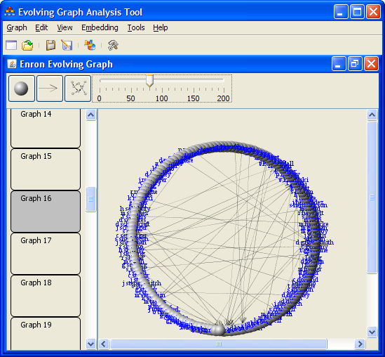
Figure 1: The interface for manipulating evolving graphs

Figure 1 shows the graphical user interface for viewing and manipulating evolving graphs. The evolving graph window, which shows an evolving graph, contains a tool bar on the top, the navigating bar on the left, and the evolving graph view on the right. The tool bar contains three buttons and a slider. Each button is used for adding new vertices, edges, or graphs respectively. The slider in the tool bar changes the scale of the evolving graph view. The navigating bar is used for selecting a graph instance in the evolving graph view. The evolving graph view also allows the user to change a vertex’s position and vertex and edge properties.

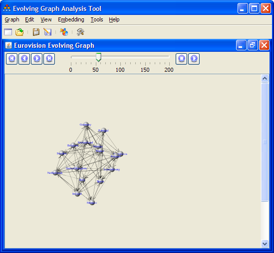
Figure 2: The interface for viewing evolving graph transitions

Figure 2 shows the graphical user interface for viewing evolving graph transitions. The transition window contains a tool bar on the top and the transition view. The tool bar contains a group of buttons used to navigate graph instances, a slider for scaling transition view, and two buttons for starting and stopping the transition.

3.3 Examples of evolving graphs

3.3.1 Eurovision dataset

The Eurovision Song Contest is an annual competition held among European countries. Each country submits a song and casts votes for the other countries’ songs, rating which ones are the best. The country with the highest score wins the competition. Broadcast since 1956, this competition is one of the most-watched non-sporting events in the world [6].

The rules of the contest have changed over time, though the current scoring system has been in use since 1975. Each participating country votes for the ten other countries by assigning the following set of points: $\{1,2,3,4,5,6,7,8,10,12\}$ [7]. Watts [16] has an interesting view on how politics affects vote results.

The Eurovision evolving graph is constructed from competition data ranging from 1956 to 2002. Each vertex represents a participating country and a directed edge represents a vote a country cast for another country. There are $47$ graph instances of undirected weighted graphs with $41$ distinct countries. The circular graph layout of Eurovision evolving graph is depicted in Figure 3.

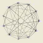
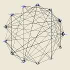
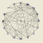
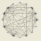
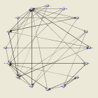
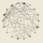
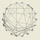
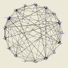
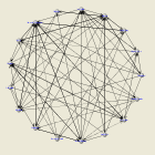
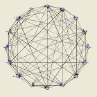
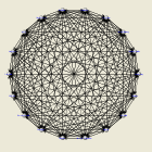
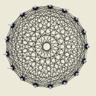
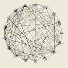
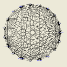
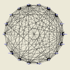
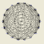
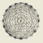
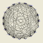
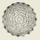
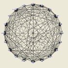
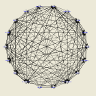
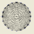
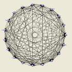
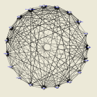
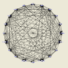
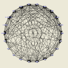
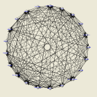
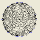
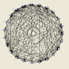
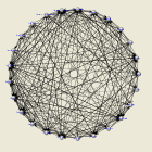
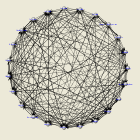
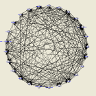
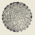
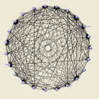
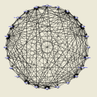
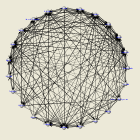
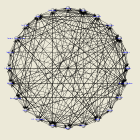
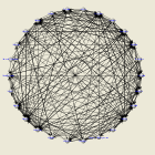
Figure 3: Eurovision evolving graph with circular layout

3.3.2 US House of Representatives dataset

The US House of Representatives dataset [9] contains roll call votes of the representatives from 1989-2004. The data are stored in text file format and each file contains roll call votes during a two-year period. The following shows sample roll call votes data:

1019990899 0USA     20000BUSH       9999996999169699999996
1011509041 1ALABAMA 20001CALLAHAN  H6616166161166616111166
1011071741 2ALABAMA 20001DICKINSON  6611166166166616666116
1011563241 3ALABAMA 10002BROWDER  GL0000000000000000000000
1011103741 3ALABAMA 10051NICHOLS  BI0000000000000000000000
1011100041 4ALABAMA 10001BEVILL  TOM1166199111616116111166
1011441941 5ALABAMA 10001FLIPPO  RON1166111111116111111116
1011502241 6ALABAMA 10001ERDREICH  B1166111111616116111166
1011541641 7ALABAMA 10001HARRIS  CLA1166111111116116111116
1011406681 1ALASKA  20001YOUNG  DONA6611611169116111966116
1011544061 1ARIZONA 20001RHODES  JOH6616166166166611661116
1011056661 2ARIZONA 10001UDALL  MORR1161111119611111116116
1011445461 3ARIZONA 20001STUMP  BOB 6616166166166616661161
1011542961 4ARIZONA 20001KYL  JON   6616166166166616666161

Each line of text contains vote results for a member of the House. The vote result, starting at column $37$ (not counting the blank spaces), can be one of the following four categories:

• $0$: Not present

• $1$: Agree

• $6$: Reject

• $9$: Present, not voting

The US house of Representatives evolving graph is constructed with each vertex representing a member of the House, each edge representing similar roll call votes between two representatives, and an edge weight representing the number of similar roll call votes. Only the vote results $1$ and $6$ are used to construct an edge.

There are $8$ graph instances of undirected weighted graphs with $443$ vertices in each graph instance. The circular graph layout of the US house of Representatives evolving graph is in Figure 4.

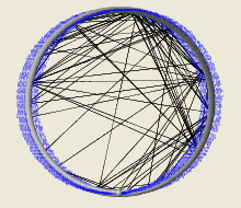
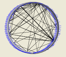
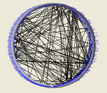
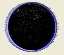
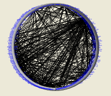
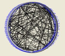
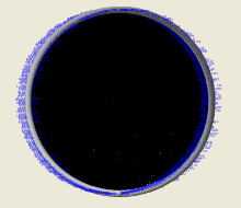
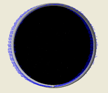
Figure 4: US House of Representatives evolving graph with circular layout

4 Graph Drawing Algorithms

4.1 Force directed algorithm

The force directed algorithm [8] is among the most common graph layout algorithms. It was designed for undirected graphs and intended to achieve the even distribution of vertices over the frame, minimizing edge crossing, making edge length uniform, and reflecting inherent symmetry.

There are two principles for graph drawing in the force directed algorithm. The first principle is to draw vertices that are connected by edges close to each other, and the second principle is that vertices should not be drawn too close to each other.

The force directed algorithm considers vertices behaving as atomic particles, exerting attractive forces and repulsive forces on one another. These attractive and repulsive forces induce movements of the vertices. The attractive force is generated between neighboring vertices and the repulsive force is generated by all vertices. These forces depend on the placement of vertices on a frame.

The total force obtained by the total sum of vectors generated by repulsive forces and attractive forces for each vertex is used to determine the new position in Displace-vertex, together with the temperature value which limits the maximum distance each vertex can move from its current position.

4.2 Vertex optimization algorithm

The Vertex optimization algorithm developed by the authors is an algorithm for drawing an evolving graph based on the force directed algorithm. It tries to optimize the vertex position to reduce the amount of movements of each vertex between the transitions. Each instance of evolving graph will be subjected to the force directed algorithm using forces generated by the graph itself and its neighboring graph instances. The vertices of the neighboring graph instances are used to generate forces that draw the same vertices on the current graph instance close to them. The outline of vertex optimization algorithm is the following.

Vertex-optimization $(EG)$
1	$\ignorespaces\mbox{\bf for\ }G\in EG$
2	do
3	$\ignorespaces\mbox{\sc Vertex-optimized-force-directed}(G)$

Vertex-optimized-force-directed $(G)$
1	$\ignorespaces\mbox{\bf for\ }i\leftarrow 1\mbox{\bf to\ }iterations$
2	do
3	$\ignorespaces\mbox{\bf for\ }u\in V$
4	do $\mbox{\bf for\ }v\in V$
5	do if $u\neq v$
6	then $\mbox{\sc Calculate-repulsive-force}(u,v)$
7	$\ignorespaces\mbox{\bf for\ }\mbox{ each edge }(u,v)\in E$
8	do $\mbox{\sc Calculate-attractive-force}(u,v)$
9	$\ignorespaces\mbox{\bf for\ }u\in V$
10	do $\mbox{\bf for\ }v\in\mbox{ neighbor of }G|u=v$
11	do $\mbox{\sc Calculate-attractive-force}(u,v)$
12	$\ignorespaces\mbox{\bf for\ }u\in V$
13	do $\mbox{\sc Displace-vertex}(u,temp)$

Vertex optimization algorithm runs Vertex-optimized-force-directed for each instance of an evolving graph. It is the same as the force directed algorithm with addition of lines 9 to 11 where it uses vertices from neighboring graph instance to calculate attractive forces between them.

Vertex $u$ is from graph instance $G$ and vertex $v$ is from neighboring graph instance of $G$. The use of attractive force to pull the same vertex on different graph instances together can be thought of as adding a new edge between them although the function for calculating attractive force may not have to be the same.

Window Size

The vertex optimization algorithm uses vertices from neighboring graph instances to determine placement of vertices. As the goal of the algorithm is to find the optimal position of vertices for each graph instance, it is not necessary to use only vertices from neighboring graph instances, which are the graph instances that are next to the considered graph instance. The more number of graph instances used, the better the vertex positions determined.

Window size is the number of graph instances that the algorithm uses to generate the attractive forces.

4.3 Vector optimization algorithm

The vector optimization algorithm, also developed by the authors, addresses the problem of making the transition between graph instances smoother by considering the direction that vertices move from and to. In vertex optimization algorithm, the goal is to minimize the distance between the same vertex on adjacent graph instances. However, in vector optimization algorithm, not only the distance is considered, but also the direction to which the vertex moves. The movement is considered smooth if the direction that the vertex moves to is somewhat the same direction. For example if a vertex moves from left to right but then moves to left, this makes the movement not smooth, since the vertex moves in the opposite direction.

The idea of vector optimization is to penalize more a vertex which has such movement by adding more force in the opposite direction.

The vector optimization algorithm constructs vectors that represent movement of vertex from vertex position of considered graph instance and its neighboring graph instances. These vectors are used to determine whether a vertex has an unsmooth movement and penalty can be assigned to the vertex. The outline for the vector optimization algorithm is as follows.

Vector-optimization $(EG)$
1	$\ignorespaces\mbox{\bf for\ }G\in EG$
2	do
3	$\ignorespaces\mbox{\sc Vector-optimized-force-directed}(G_{p},G,G_{n})$

Vector-optimized-force-directed $(G_{p},G,G_{n})$
1	$\ignorespaces\mbox{\bf for\ }i\leftarrow 1\mbox{\bf to\ }iterations$
2	do
3	$\ignorespaces\mbox{\bf for\ }u\in V$
4	do $\mbox{\bf for\ }v\in V$
5	do if $u\neq v$
6	then $\mbox{\sc Calculate-repulsive-force}(u,v)$
7	$\ignorespaces\mbox{\bf for\ }\mbox{ each edge }(u,v)\in E$
8	do $\mbox{\sc Calculate-attractive-force}(u,v)$
9	$\ignorespaces\mbox{\bf for\ }u\in V$
10	do $u_{p}\in V_{p}|u=u_{p}$
11	$\ignorespaces u_{n}\in V_{n}|u=u_{n}$
12	$\ignorespaces\nu_{1}=\mbox{\sc construct-vector}(u_{p},u)$
13	$\ignorespaces\nu_{2}=\mbox{\sc construct-vector}(u,u_{n})$
14	$\ignorespaces\nu_{a}=\nu_{1}+\nu_{2}$
15	if $|\nu_{a}|<\mbox{max}(\nu_{1},\nu_{2})$
16	then $\mbox{\sc Calculate-attractive-force}(u,v,penalty)$
17	else  $\mbox{\sc Calculate-attractive-force}(u,v)$
18	$\ignorespaces\mbox{\bf for\ }u\in V$
19	do $\mbox{\sc Displace-vertex}(u,temp)$

The Vector optimization algorithm runs Vector-optimized-force-directed
for each instance of an evolving graph. It is the same as the force directed algorithm with addition of lines 9 to 17. It has parameters $G_{p}$, $G$, and $G_{n}$ where $G_{p}$ denotes a graph $G_{p}=(V_{p},E_{p})$ as the previous graph instance, $G$ denotes a graph $G=(V,E)$ as the current graph instance, and $G_{n}$ denotes a graph $G_{n}=(V_{n},E_{n})$ as the next graph instance.

Vectors $\nu_{1}$, $\nu_{2}$ and $\nu_{a}$ are created from the position of vertex $u$ on different graph instances. Vector $\nu_{1}$ is created from the position of vertex $u_{p}$, the vertex $u$ on the previous graph instance and vertex $u$. Vector $\nu_{2}$ is created from the position of vertex $u$ and vertex $u_{n}$, the vertex $u$ on the next graph instance. Vector $\nu_{a}$ is the vector addition of vector $\nu_{1}$ and $\nu_{2}$.

The condition for penalizing a vertex with more force to the opposite direction is $\nu_{a}<\mbox{max}(\nu_{1},\nu_{2})$, the addition of two vectors has a size smaller than either of $\nu_{1}$ or $\nu_{2}$. This is because the size of the vector addition will increase if two vectors are in about the same direction and the size will decrease if two vectors are not in the same direction. The penalized force is computed when the condition holds true in Calculate-attractive-force. By adding a $penalty$ value, the force in opposite direction is computed.

4.4 Measurement for optimization

The goal for optimization is to place vertices in a way that minimizes their movements. An obvious parameter for optimization is the total distances these vertices move. The total distances can be measured in different way depending on whether the interest is in the overall performance, the specific vertex, or specific graph.

Total distance measurement ( $td_{EG}$ )

Total distance measurement adds the movements of all vertices during the transition for all graph instances. The total distance measurement of an evolving graph can be computed as follows:

Total-distance $(EG)$
1	$\ignorespaces td_{EG}\leftarrow 0$
2	$\ignorespaces\mbox{\bf for\ }i\leftarrow 1\mbox{\bf to\ }p-1$
3	do
4	$\ignorespaces G_{i}=(V_{i},E_{i})\in EG$
5	$\ignorespaces G_{i+1}=(V_{i+1},E_{i+1})\in EG$
6	$\ignorespaces\mbox{\bf for\ }u_{i,j}\in V_{i}$
7	do $\mbox{\bf for\ }u_{i+1,j}\in V_{i+1}$
8	do $td_{EG}\leftarrow td_{EG}+d(u_{i,j},u_{i+1,j})$
9	$\ignorespaces\mbox{\bf return\ }td_{EG}$

Total distance per graph measurement ( $td_{G}$ )

Total distance per graph measurement sums all the movements of vertices during the transition from graph instance $G$ to the next graph instance. It can be computed as follows:

Total-distance-per-graph $(G,EG)$
1	$\ignorespaces td_{G}\leftarrow 0$
2	$\ignorespaces G=(V,E)\in EG$
3	$\ignorespaces G_{n}=(V_{n},E_{n})\in EG|G_{n}\mbox{ is the next graph instance from }G$
4	$\ignorespaces\mbox{\bf for\ }u_{j}\in V$
5	do $\mbox{\bf for\ }u_{n,j}\in V_{n}$
6	do $td_{G}\leftarrow td_{G}+d(u_{j},u_{n,j})$
7	$\ignorespaces\mbox{\bf return\ }td_{G}$

Total distance per vertex measurement ( $td_{v}$ )

Total distance per vertex measurement sums all the movements of a vertex during the transition for all graph instances. It can be computed as follows:

Total-distance-per-vertex $(v,EG)$
1	$\ignorespaces td_{v}\leftarrow 0$
2	$\ignorespaces\mbox{\bf for\ }i\leftarrow 1\mbox{\bf to\ }p-1$
3	do
4	$\ignorespaces G_{i}=(V_{i},E_{i})\in EG$
5	$\ignorespaces G_{i+1}=(V_{i+1},E_{i+1})\in EG$
6	$\ignorespaces\mbox{\bf for\ }u_{i,j}\in V_{i}$
7	do $\mbox{\bf for\ }u_{i+1,j}\in V_{i+1}$
8	do $td_{v}\leftarrow td_{v}+d(u_{i,j},u_{i+1,j})$
9	$\ignorespaces\mbox{\bf return\ }td_{v}$

5 Experimental results

The Vertex optimization and Vector optimization algorithms were run on different types of evolving graphs. First, vertex optimization was run on generated evolving graphs which are randomly generated evolving graphs with different degree distribution. Second, vertex optimization was run on five evolving graphs. These evolving graphs were created specifically to understand the effect of the algorithm on evolving graphs. Third, the comparison between vertex optimization and vector optimization was done with evolving graphs. Fourth, vertex optimization algorithm was run on real-world evolving graphs such as Eurovision evolving graphs and US House of Representatives evolving graphs.

5.1 Vertex optimization on generated evolving graphs

In this experiment, the vertex optimization algorithm is tested on different types of generated evolving graphs. The effect of window size and performance is also tested.

Three types of generated evolving graphs are used, namely, random evolving graphs, exponential evolving graphs and scale-free evolving graphs. These evolving graphs have their graph instances with different degree distribution. Random evolving graphs are constructed such that their graph instances have Poisson degree distribution. Exponential evolving graphs have graph instances with exponential degree distribution. And scale-free evolving graphs have graph instances with power-law degree distribution.

All evolving graphs are constructed with comparable size. There are 20 graph instances in total where the first graph instance for random evolving graphs has 50 vertices and 20 edges and 5 more edges are added to each graph instance to create the next graph instance.

For exponential and scale-free evolving graphs, the first graph instance has 31 vertices and one more vertex is added for the next graph instance. Therefore the last graph instance will also have 50 vertices which is the same as number of vertices for random evolving graphs.

These generated evolving graphs are tested with the vertex optimization algorithm with different window size and the total distance measurement ( $td_{EG}$ ) is measured.

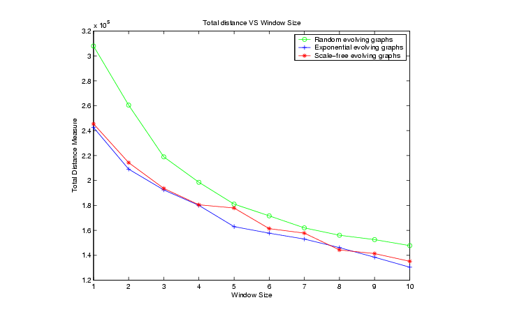
Figure 5: The total distance measure with different window size on different types of evolving graphs

Figure 5 shows the plot of total distance measure versus varying window size after applying vertex optimization algorithm on the evolving graphs. The different types of evolving graphs are shown as different plots. All types of evolving graphs have the same effect as the total distance decreases when the window size increases. This means with higher window size value the movement distance of vertices become shorter.

Window size indicates the number of graph instances that are used to compute vertex placement and therefore the larger the window size the more the information available for determining the vertex placement.

The random evolving graphs also have higher total distance value than the other two evolving graphs. This is predictable considering the number of vertices the random evolving graphs have. Random evolving graphs have fixed number of vertices for all graph instances and have more vertices than the other two evolving graphs. These additional vertices must contribute to the higher total distance measure.

The exponential evolving graphs and scale-free evolving graphs have the same number of vertices and the total distance measure is about the same.

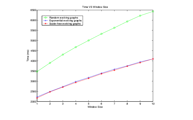
Figure 6: The computation time with different window size on different types of evolving graphs

Figure 6 shows the plot of computation time versus varying window size. The plot shows that large window size requires more computation time than small window size. The computation times for random evolving graphs are higher than the other two evolving graphs, also because of the number of vertices as in Figure 5. These two plots show the trade-off between the optimized vertex position and computation time when changing window size. With larger window size, a better vertex position can be obtained at the expense of more computation time.

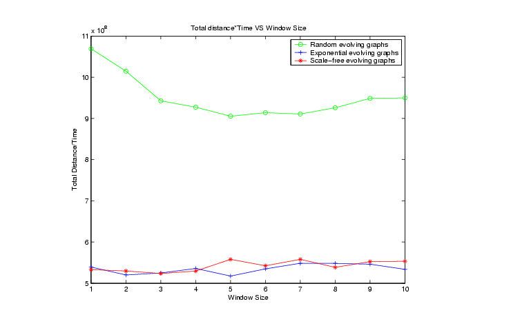
Figure 7: The total (distance * computation) time with different window size on different types of evolving graphs

Figure 7 shows the plot of total distance measure times the computation time versus varying window size. The value represents the performance trade-off between the optimal position and computation time. The lower value for total distance and computation time is preferable; therefore, the lowest point of the plot will represent the optimal window size. For random evolving graphs, the plot clearly shows the optimal window size at 5. The other plots have no clear optimal window size as the plots are almost straight lines.

This suggests that for random evolving graphs the best window size is around 5 but for real-world evolving graphs which have exponential or power-law distribution, choosing the window size depends more on the trade-off between the cost and computation time i.e., if we are more concerned about the cost, the larger window size is better, and if computation time is more important then lower window size is better.

5.2 Vertex optimization on evolving graphs

More examples of evolving graphs are constructed to understand the vertex optimization algorithm. All the evolving graphs have twenty graph instances and are described below.

Example: Evolving graph 1

Each instance is a line graph with 53 vertices and edges $(i,i+1)|\forall i=1..52$.

Evolving graph 1 is a line graph with no change between graph instances. All the vertices remain unchanged in position in different graph instances. Figure 8 shows one graph instance of evolving graph 1.Only the first five vertices of the graph instance are shown.

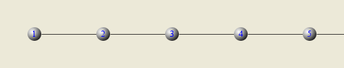
Figure 8: Portion of evolving graph 1

Example: Evolving graph 2

The odd instances are line graphs with 53 vertices and edges $(i,i+1)|\forall i=1..52$. The even instances are graphs with 53 vertices and no edges.

Evolving graph 2 has graph instances which switch between a line graph and a graph with no edges. All vertices remain unchanged in position in different graph instances. Figure 9 shows two graph instances in evolving graph 2. The odd graph instance is on top and the even graph instance is on the bottom in the figure. Only the first five vertices of each graph instance are shown.

Figure 9: Portion of evolving graph 2

Example: Evolving graph 3

The first 15 instances are line graphs with 53 vertices and edges $(i,i+1)|\forall i=1..52$. The last 5 instances are line graphs with 53 vertices and edges $(i,(i+2)\%53)|\forall i=1..51,53$.

Evolving graph 3 has two sets of line graphs. The first set has 15 graph instances and the other set has 5 graph instances. The setup for the second set of graph instances has different vertices in the same position as vertices in the first set of graph instances, e.g., vertex 1 is in the same position for both sets, vertex 2 from the first set is in the same position as vertex 3 from the second set and so on. Figure 10 shows two graph instances in evolving graph 3. The first 15 graph instances are the same as the top figure and the last 5 graph instances are the same as the bottom figure. Only the first five vertices of each graph instance are shown.

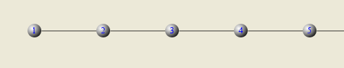
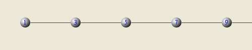
Figure 10: Portion of evolving graph 3

Example: Evolving graph 4

Each graph instance has 53 vertices. The $k^{th}$ graph instance contains edges $(i,(i+k)\%53)|\forall i=1..(53-k)$.

Evolving graph 4 has twenty different sets of line graphs. The first line graph has vertices in the order 1, 2, 3, and so on. The second line graph has vertices in the order 1, 3, 5, and so on. Different vertices from different graphs are in the same position, i.e., vertex 1 is in the same position for all graph instances, vertex 2 from the first graph instance, vertex 3 from the second graph instance, vertex 4 from the third graph instance are in the position. Figure 11 shows the first five graph instances in evolving graph 4. Only the first five vertices are shown in each graph instance.

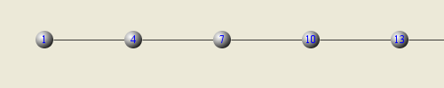
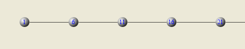
Figure 11: Portion of evolving graph 4

Example: Evolving graph 5

Each graph instance is a circular graph with 53 vertices and edges $(i,i+1)|\forall i=1..53$ and extra edges $(40,j)|\forall j=1..20$ but the edge $(40,k)$ for the $k^{th}$ graph instance is absent.

Evolving graph 5 has twenty circular graph instances with additional edges from vertex 40 to a set of vertices 1 to 20. One additional edge is missing for each graph instance. All the same vertices in different graph instances are in the same position. Figure 12 shows the first four graph instances in evolving graph 5.

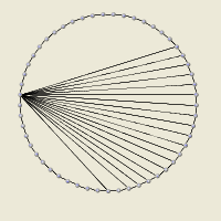
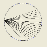
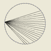
Figure 12: Portion of evolving graph 5

Experimental results

Each evolving graph is run on the vertex optimization algorithm using different window sizes from 1 to 5. The results are quantified by distance measure and plotted in Figure 21 to 35 in Appendix A.

5.3 Vertex optimization Vs. Vector optimization algorithm

The five evolving graphs have been used to compare the two evolving graph layout algorithms.

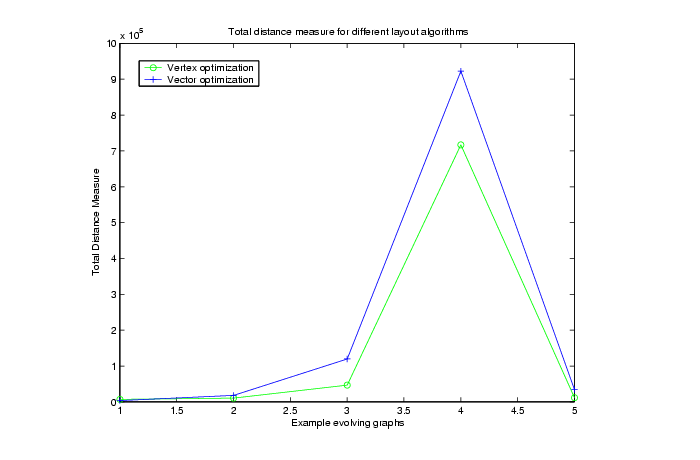
Figure 13: The total distance measure with different layout algorithms

Figure 13 shows the comparison of total distance measure between vertex optimization and vector optimization algorithms. The window size is set to five for both algorithms. The plot shows that vector optimization algorithm does not improve over the vertex optimization algorithm.

5.4 Vertex optimization on Eurovision and US House of Representatives evolving graphs

Eurovision evolving graph

The circular graph layout of Eurovision evolving graph is in Figure 3. This layout gives a general view of each graph instance in the Eurovision evolving graph. The first 14 graph instances have smaller number of vertices and edges than the other instances. This is attributed to the change in competition format which results in more consistent number of participating countries and scores each country gives to the others.

The graph layout of Eurovision evolving graph using vertex optimization algorithm is in Figure 14. The winning country in each year is represented by the red vertex in the drawing. These winning countries, in general, are placed not far from the center of the graph. Although we expect them to be exactly at the center of the graph, that is not the case, which is due to several reasons. First, the competition should be modeled as a weighted directed graph, but vertex optimization does not take edge weight into account. Second, vertex optimization has window size effect which pulls the same vertex in different graph instance together.

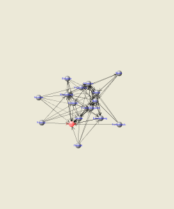
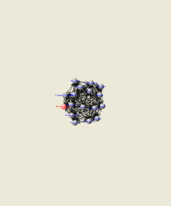
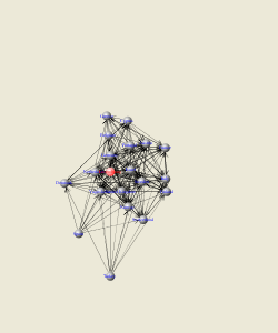
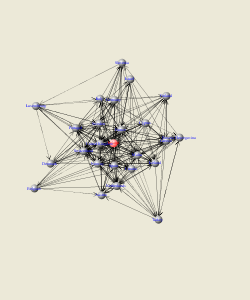
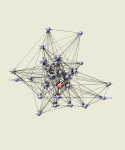
Figure 14: Eurovision evolving graph with vertex optimization layout

The total distance measure for Eurovision evolving graph is as follows:

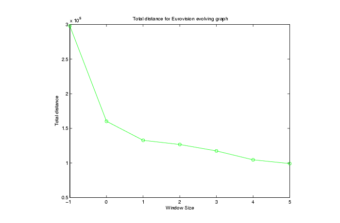
Figure 15: The total distance measure with different window sizes on Eurovision evolving graph

Figure 15 shows the plot of total distance measure versus varying window sizes on the Eurovision evolving graph. Another two values are added to the plot at window sizes of -1 and 0. The first value describes the total distance when the vertices on Eurovision evolving graph are placed randomly. The second value describes the total distance when the algorithm does not use any information from neighboring graph instances. It is equivalent to running a force directed algorithm on each graph instance separately. Overall, the vertex optimization helps reduce the movement of vertices for Eurovision graphs, the larger the window size, the smaller the total distance measure.

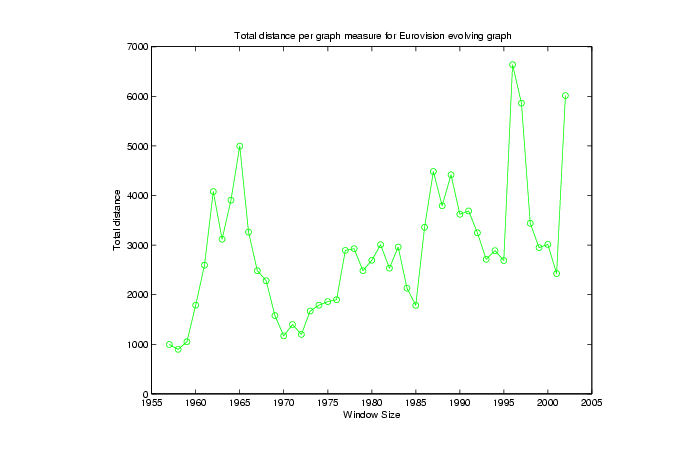
Figure 16: The total distance measure per graph on Eurovision evolving graph

Figure 16 shows the plot of total distance measure per graph on Eurovision evolving graph. There are spikes in the plot which is consistent with graph difference.

Country	Total distance	No.	Avg total distance
Italy	2215	31	71.45
United Kingdom	3390	44	77.05
Germany	3745	44	85.12
Switzerland	3327	39	85.30
France	3877	42	92.32
Sweden	3614	39	92.67
Romania	95.71	1	95.71
Monaco	1929	20	96.47
Denmark	2859	27	105.89
Netherlands	4133	38	108.77
Luxembourg	3781	34	111.21
Estonia	798	7	114.02
Yugoslavia	2813	24	117.24
Lithuania	117	1	117.99
Ireland	4062	34	119.48
Belgium	4838	40	120.95
Austria	4273	35	122.10
Spain	5431	42	129.31
Norway	5338	39	136.87
Finland	4386	31	141.48
Israel	3017	21	143.70
Malta	1942	13	149.44
Russia	657	4	164.48
Slovenia	1065	6	177.51
Greece	3212	18	178.49
Croatia	1930	10	193.06
Cyprus	3610	18	200.59
Turkey	4262	21	202.96
Iceland	2773	13	213.36
Poland	1080	5	216.02
Portugal	7370	33	223.34
Bosnia Herzegovina	1431	6	238.59
Latvia	898	3	299.65
Hungary	811	2	405.59
FYR Macedonia	0	0	0
Morocco	0	0	0
Slovakia	0	0	0
Ukraine	0	0	0

Table 1: Total distance per vertex for each country sorted by average total distance

Table 1 shows the total distance per vertex for each country of Eurovision evolving graph. Since some countries do not participate every year, the average total distances per vertex are calculated. The list of countries is sorted by this average. Italy, United Kingdom, Germany, Switzerland, France and Sweden are the six smallest movement countries. Hungary, Latvia, Bosnia Herzegovina, Portugal and Poland are the largest movement countries. FYR Macedonia, Morocco, Slovakia, and Ukraine are countries that never participate in consecutive year so the total distance are not measured.

Countries with small movements are consistent with countries that form a cluster. The total distance per vertex could be another way to determine a cluster in evolving graphs.

US House of Representatives evolving graph

The circular graph layout of US House of Representatives evolving graph is in Figure 4. This layout shows the density of edges in each graph instance. The $4^{th}$, $7^{th}$, and $8^{th}$ graph instances have high edge density even though edges have been filtered by $90\%$ weight threshold.

The graph layout of US House of Representatives evolving graph using vertex optimization algorithm is in Figure 17. Due to very large layout, vertices in the drawing appear as small dots. A giant component can be seen in all graph instances. We expect to see two giant components representing two parties and the layouts show one bigger giant component and a smaller component. The reason the second component cannot be seen clearly is because of the weight threshold. The graph instances in which the second component cannot be seen clearly just do not have enough edges for the second component to form. The graph instances that have high density edges clearly shows two giant components.

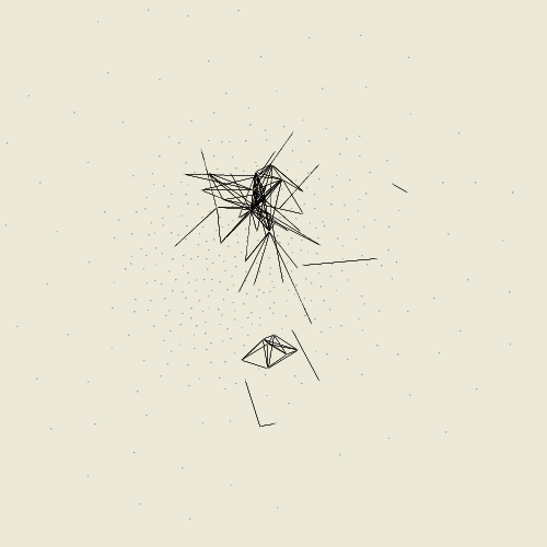
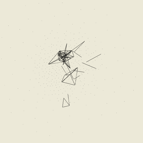
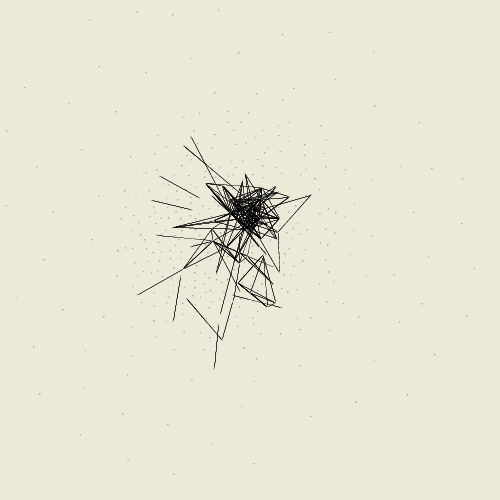
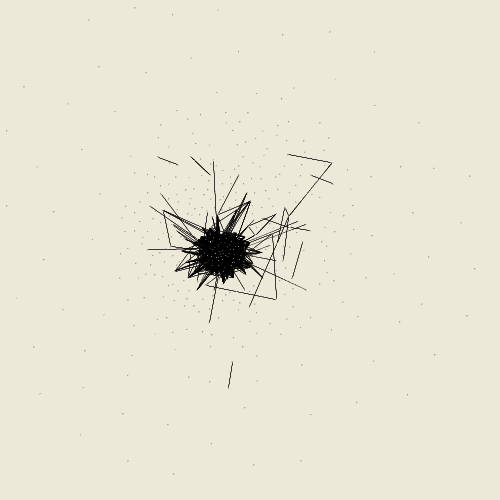
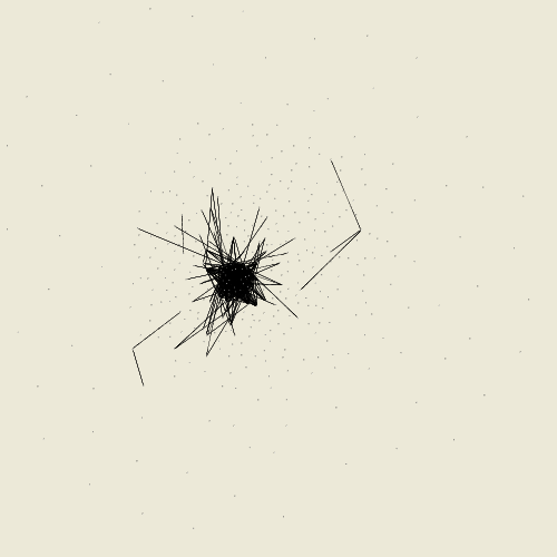
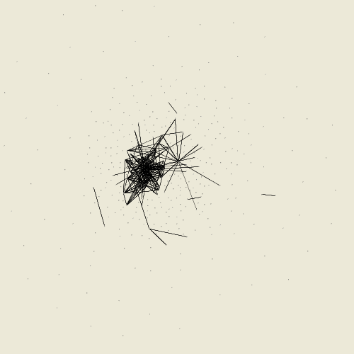
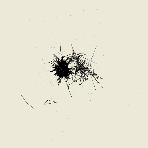
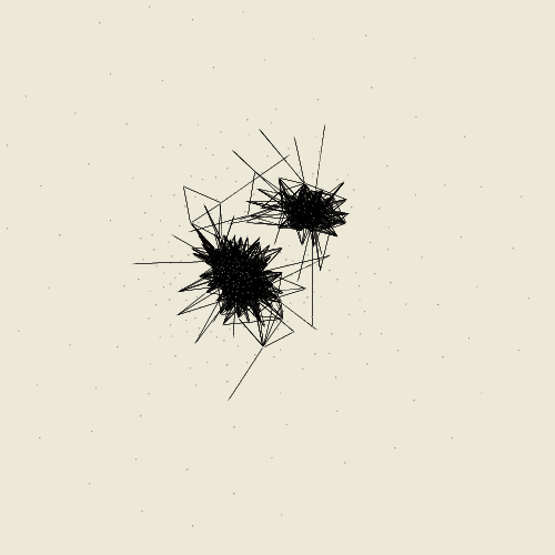
Figure 17: US House of Representatives evolving graph with vertex optimization layout

The total distance measure for Eurovision evolving graph is as follows:

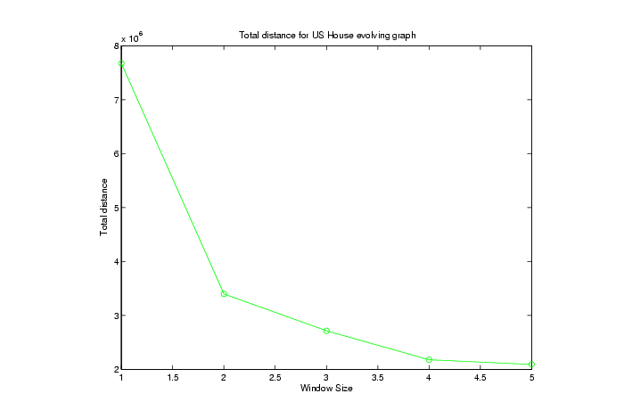
Figure 18: The total distance measure on US House of Representatives evolving graph

Figure 18 shows the total distance measure on US House of Representatives evolving graph with different window sizes. The total distance drops, as the window size increases.

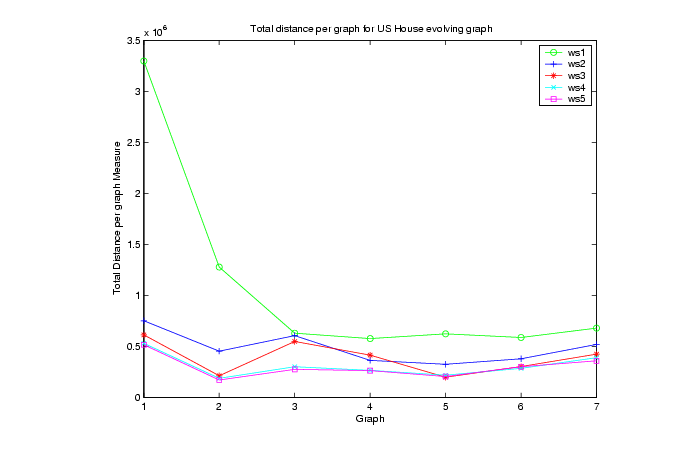
Figure 19: The total distance measure per graph on US House of Representatives evolving graph

Figure 19 shows the total distance per graph measure on US House of Representatives evolving graph. For window sizes higher than one, the total distance measure per graph are quite steady through all graph instances, suggesting that there is no significant difference in graph configuration.

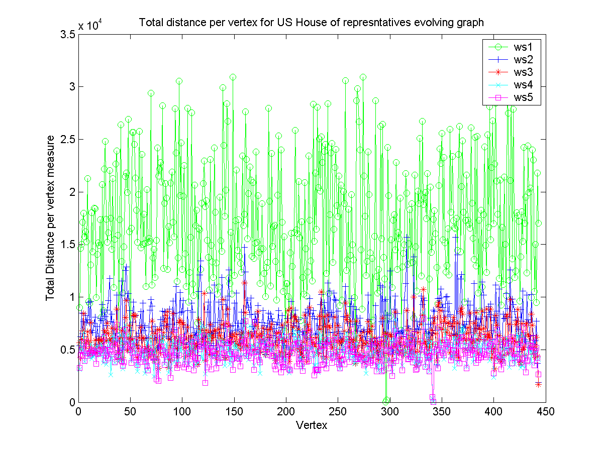
Figure 20: The total distance measure per vertex on US House of Representatives evolving graph

Figure 20 shows the total distance per vertex measure on US House of Representatives evolving graph. The average total distance per vertex is also calculated. The average value is in the range 265 to 1138. George Bush is in the $42^{th}$ place with average value of 470.

6 Conclusions

The goal for an evolving graph layout algorithm in the current work is to automatically draw an evolving graph in two dimensions in a manner that augments intuitive understanding of an evolving graph. This involves drawing graph instances to reflect their structure and also providing smooth transitions between graph instances.

Two new evolving graph layout algorithms are introduced and analyzed as part of a research study on visualization tools for evolving graphs. The first algorithm, the vertex optimization algorithm, minimizes the distance between the same vertex in neighboring graph instances by extending the force directed graph layout algorithm. It incorporates attractive forces between the same vertices on neighboring graph instances with the existing forces in force directed algorithm. The second algorithm, the vector optimization algorithm, addresses the smooth movement of vertices between transitions between graph instances. Forces are increased as a penalty for vertices which unsmooth the transitions.

Three measurements are introduced for capturing vertex movements. The total distance explains the overall performance of a layout algorithm. The total distance per graph explains the movement between graph instances as well as the difference between their graph instances’ structure. The total distance per vertex explains the impact of different graph instances’ structure upon a vertex.

Different types of evolving graphs are tested using vertex optimization algorithm. The experiments show that the difference in degree distribution does not affect the total distance as much as the difference in graph structure. Window size, which indicates the amount of information a certain graph instance can gather from its neighboring graph instances, has a significant impact on the total distance measure. However, this comes with a trade-off with computation time. A good window size for small to medium size evolving graphs is five.

Although vector optimization algorithm looks promising to provide a smoother transition between graph instances, the experiments show that there is no improvement over vertex optimization in terms of the total distance measure.

Experiments on real data evolving graphs also show that vertex optimization algorithm can minimize the total movements for vertices in these evolving graphs, thereby giving a smoother transition. The three total distance measurements can be used together with other analysis tools such as clustering, or centrality metrics.

Appendix A

Figures 21 to 36

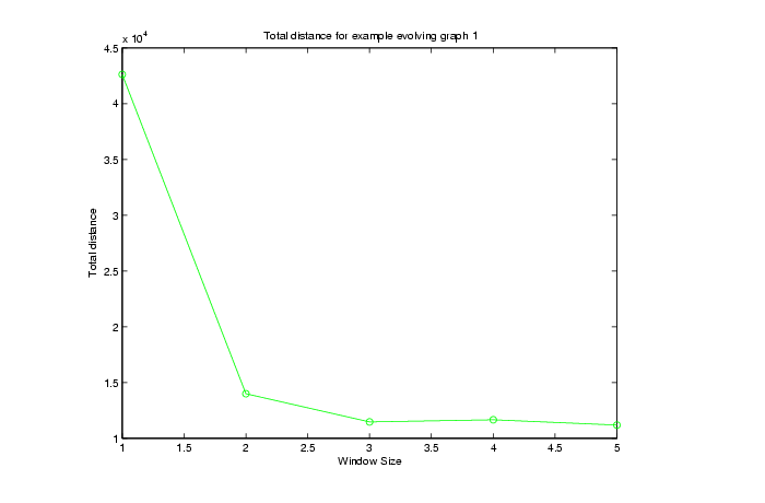
Figure 21: The total distance measure with different window sizes on evolving graph 1

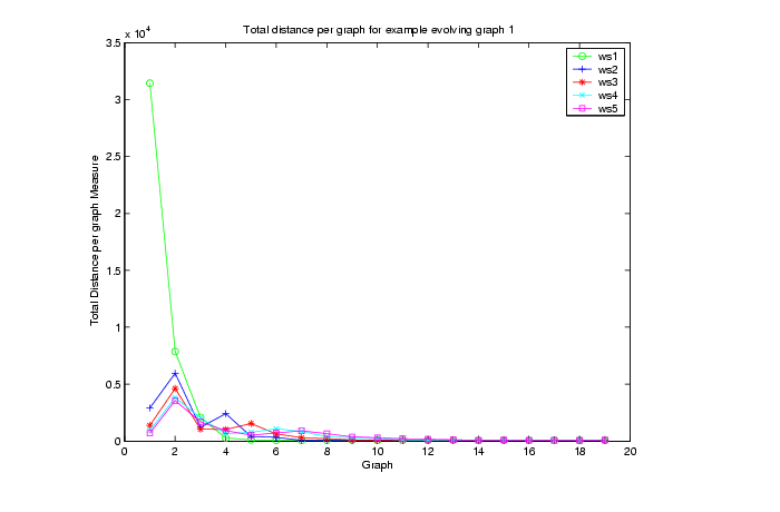
Figure 22: The total distance per graph measure with different window sizes on evolving graph 1

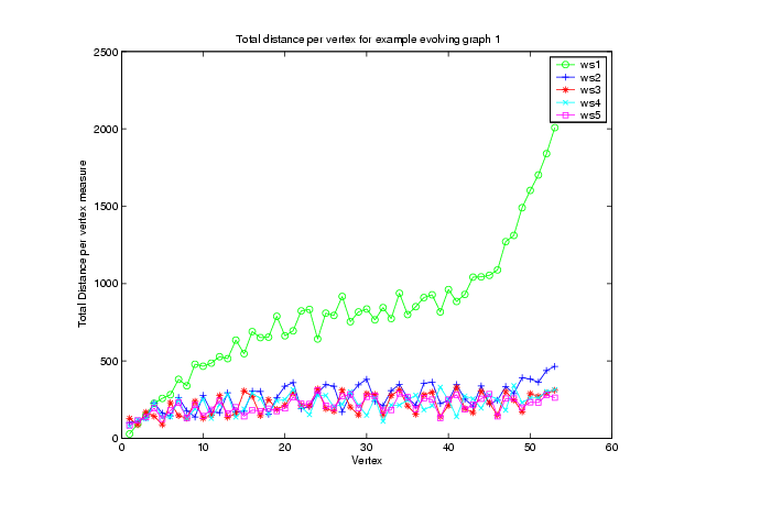
Figure 23: The total distance per vertex measure with different window sizes on evolving graph 1

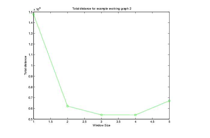
Figure 24: The total distance measure with different window sizes on evolving graph 2

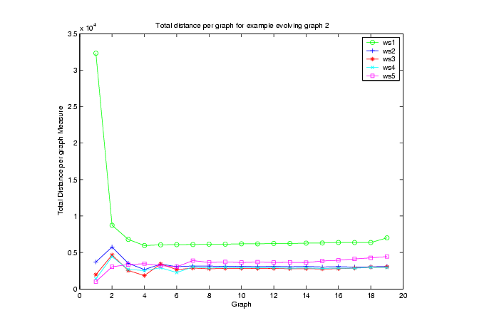
Figure 25: The total distance per graph measure with different window sizes on evolving graph 2

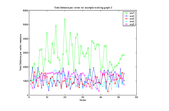
Figure 26: The total distance per vertex measure with different window sizes on evolving graph 2

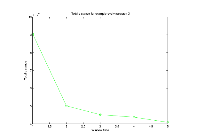
Figure 27: The total distance measure with different window sizes on evolving graph 3

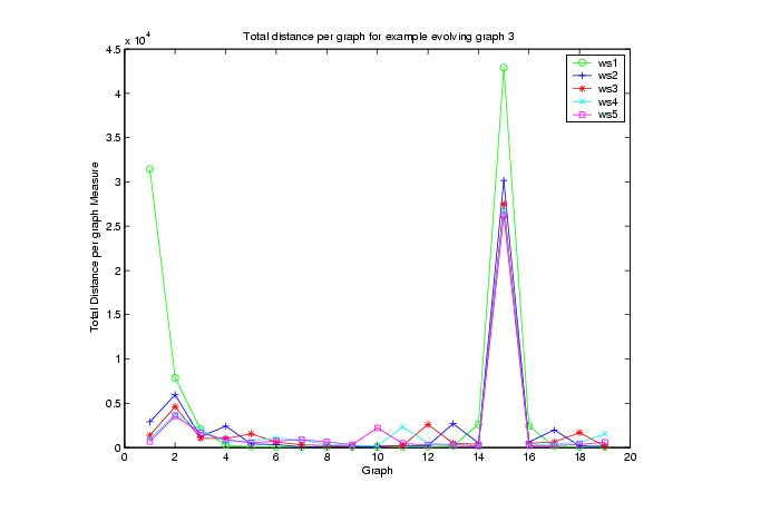
Figure 28: The total distance per graph measure with different window sizes on evolving graph 3

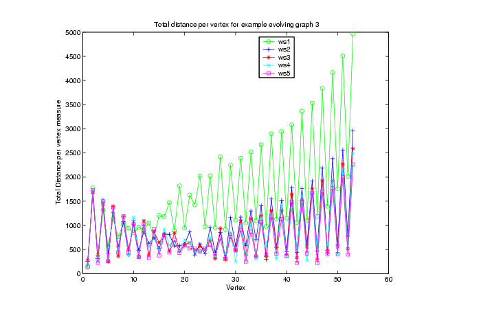
Figure 29: The total distance per vertex measure with different window sizes on evolving graph 3

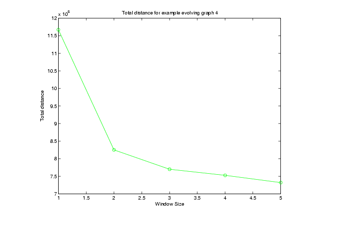
Figure 30: The total distance measure with different window sizes on evolving graph 4

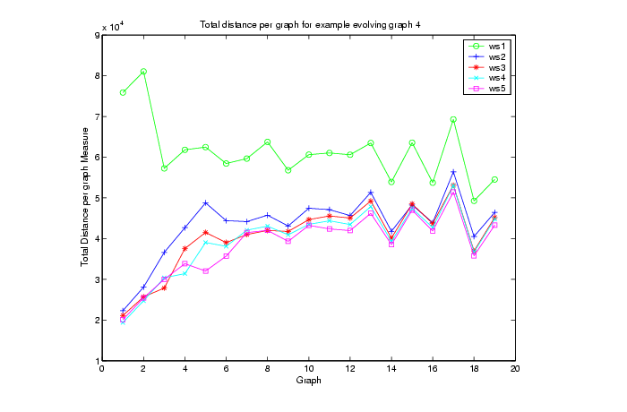
Figure 31: The total distance per graph measure with different window sizes on evolving graph 4

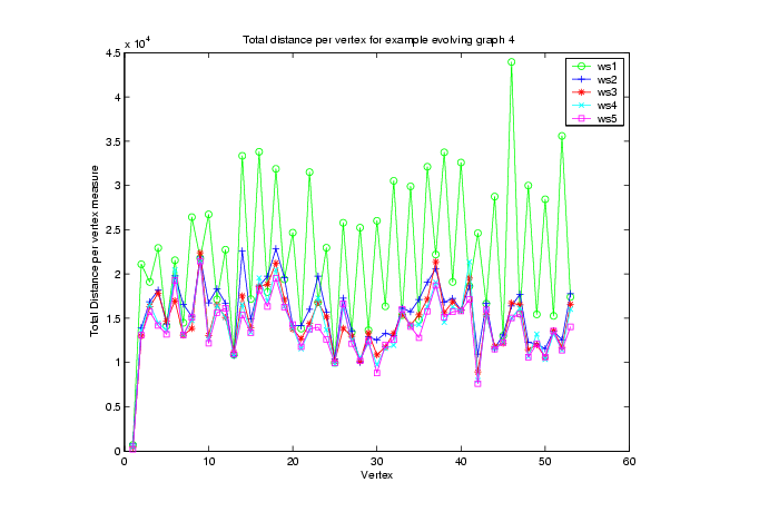
Figure 32: The total distance per vertex measure with different window sizes on evolving graph 4

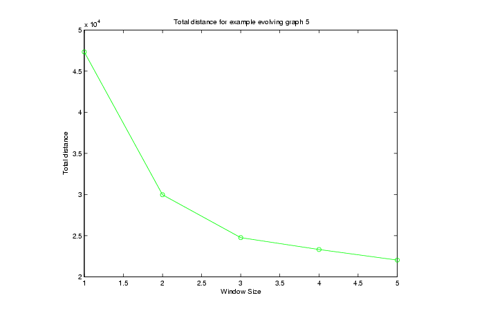
Figure 33: The total distance measure with different window sizes on evolving graph 5

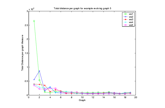
Figure 34: The total distance per graph measure with different window sizes on evolving graph 5

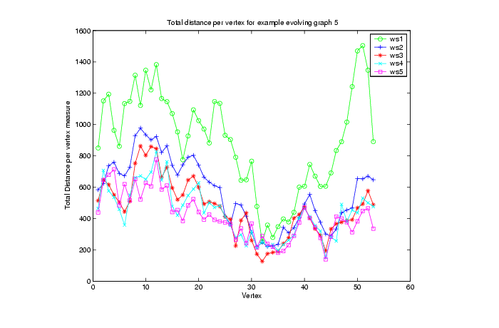
Figure 35: The total distance per vertex measure with different window sizes on evolving graph 5

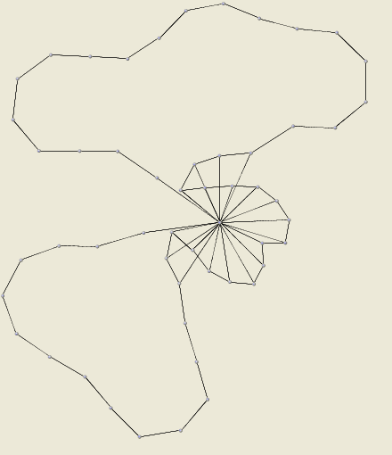
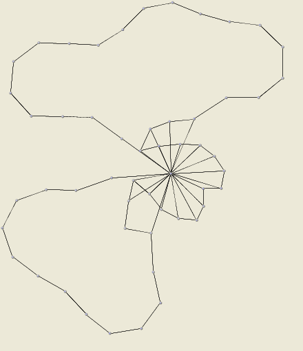
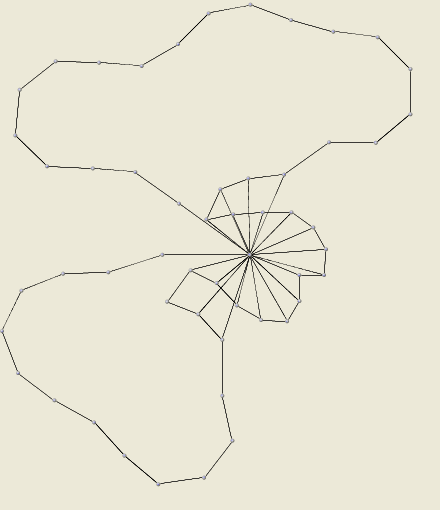
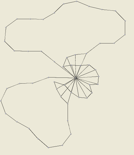
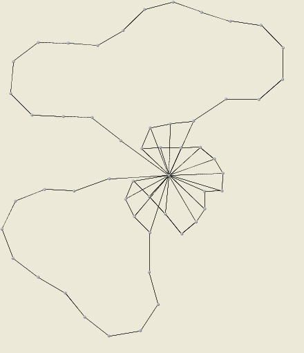
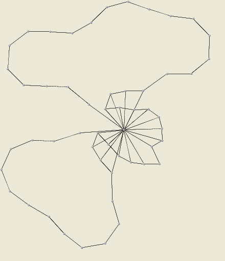
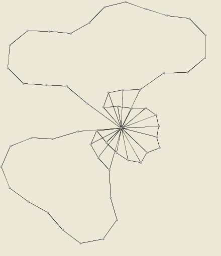
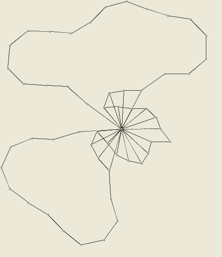
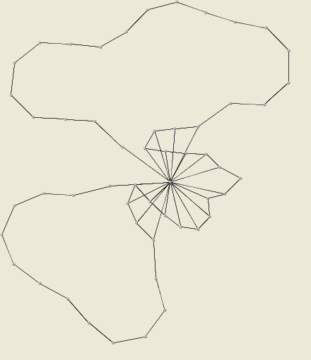
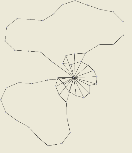
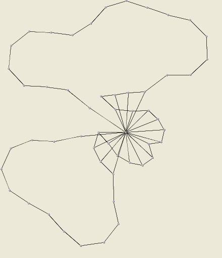
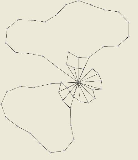
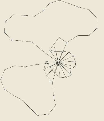
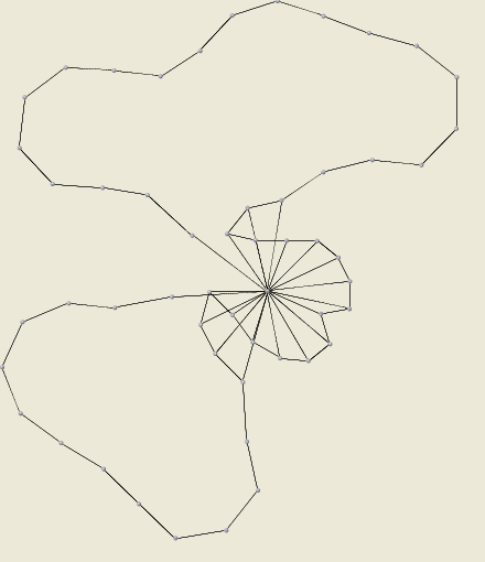
Figure 36: Example evolving graph 5 with vertex optimization layout

Discussion

Figures 21, 24, 27, 30, and 33 show the total distance measure with window size from one to five on evolving graphs 1 to 5, respectively. Figures 22, 25, 28, 31, and 34 show the total distance per graph measure with window size from one to five on evolving graphs 1 to 5, respectively. Figures 23, 26, 29, 32, and 35 show the total distance per vertex measure with window size from one to five on evolving graphs 1 to 5, respectively.

In Figure 21 the plot of total distance measure drops from window size of 1 to 2 and is quite steady afterward. This suggests that window size of 1 is not big enough and after window size of 2, there is small gain on improvement.

Figure 22 shows that most of the total distance per graph measure for window size of 1 comes from the difference between the first and second graph instance. All window sizes have high total distance per graph between the second and third graph instances. The figure shows that the first couple of graph instances are in unsteady state because the force directed algorithm moves vertices in the first graph instance further in the early round, but are unable to move them back since the first graph instance is constrained by other graph instances which are still not in their optimized position; contrary to the other graph instances which are constrained by some optimized graph instances, which, therefore, are likely to be in a more steady state.

Figure 23 shows that total distance per vertex measure on evolving graph 1 with window size of 1 keeps increasing for later vertices where other window size have steady total distance measure for all vertices. This suggests that the vertices are moved away further at the end of a line graph.

Figure 24 is a plot of total distance measure on evolving graph 2. It shows the drop as window size increases. However, the total distance measure is significantly higher than the plot of evolving graph 1.

In Figure 25, the plot of total distance measure per graph on evolving graph 2 with window size 1 shows higher total distance than the other window sizes for all graph instances. The plot also shows the same effect between graph instance 2 and 3 as in Figure 22.

In Figure 26, the plot of total distance measure per vertex on evolving graph 2 shows varying total distance between vertices. This shows that all the vertices are disturbed by the configuration of switching between two sets of graph instances.

In Figure 27, the plot of total distance measure on evolving graph 3 shows the drop as window size increases. The total distance measure is higher than that of evolving graph 1.

In Figure 28, the plot of total distance measure per graph on evolving graph 3 shows the high total distance measure between the two graph instance with different configurations, which is expected. It is significant to point out that another high total distance occurs at another graph instance far from the highest total distance by the amount of window size. For example, with window size of 4, the highest total distance is at graph 15; graphs 11 and 19 also have high total distance.

In Figure 29, the plot of total distance measure per vertex on evolving graph 3 has an interesting pattern. The odd vertices seem to have low total distance and the even vertices have high total distance. From the configuration, this is reasonable because the first set of graph instances connects the odd and even vertices together and the second set of graph instances connects the odd vertices with odd vertices and the even vertices with even vertices.

In Figure 30, the plot of total distance measure on evolving graph 4 has the same shape as that of other evolving graphs. The total distance value, however, is significantly higher than the other evolving graphs. Since all graph instances have different configurations, this is expected.

In Figure 31, the plot of total distance measure per graph on evolving graph 4 shows high total distance for all graph instances for all window sizes. Window sizes 2 to 5 all have a comparatively similar plot. The configuration is set up so that the same vertex is farther for later graph instances. Therefore, the plot increases from graph instance 1 to 5. After graph instance 5, with the roundup, the vertices are no farther any more and total distance stops increasing.

In Figure 32, the plot of total distance measure per vertex on evolving graph 4 shows high total distance for window size of 1. Window sizes 2 to 5 have comparatively similar plots.

In Figure 33, the plot of total distance measure on evolving graph 5 drops as the window size increases.

In Figure 34, the plot of total distance measure per graph on evolving graph 5 shows unsteady state in the first couple of graph instances and steady state afterward for all window sizes. The difference of one edge seems to have little impact on the overall placement.

In Figure 35, the plot of total distance measure per vertex on evolving graph 5 shows varying total distance for each vertex. Vertex 40 with the most changes has high total distance but does not have the highest total distance. Vertices 1 to 20 which connect to vertex 40 all have high total distances. The plot around vertices 1 to 20 looks like a bell curve and the plot around vertex 40 looks like a spike. This suggests that vertices around the high total distance vertices are pulled. This is reasonable because the graph configuration is circular. The graph layout using vertex optimization algorithm for evolving graph 5 is in Figure 36.

Overall, the results show that for simple evolving graphs such as example 1 and example 2, where the best result is to retain the position of all vertices, the vertex optimization algorithm might not obtain the best result. However, considering other factors such as the optimum position of vertices relative to other vertices in the same graph instances that the force directed algorithm provides, the vertex optimization algorithm can be used for automatic evolving graph layout.

Different window sizes yield different results with high value of window size generally resulting in better total distance measure. Window size 1 gives poor results compared to others and window size 2 is adequate for very simple evolving graphs.

Evolving graph 1 shows that error in the first few graph instances contributes to the total distance measure. Evolving graph 2 shows that the difference in graph configuration contributes to the total distance measure. Evolving graphs 3, 4 and 5 show that the total distance per graph measure can tell roughly where the high change in graph configuration occurs. Total distance per vertex measure can explain the difference in graph configuration.

Appendix B

EGML DTD Specifications

<!-- DTD for EGML 1.0 -->
<!-- Authors: Anurat Chapanond -->
<!-- Computer Science Department -->
<!-- Rensselaer Polytechnic Institute -->
<!-- egml.dtd,v 1.0 03/16/2007 -->

<!-- Boolean type -->
<!ENTITY % boolean.type "(0|1)" >

<!-- Positive number type -->
<!ENTITY % number.type "NMTOKEN">

<!-- ID type -->
<!ENTITY % id.type "NMTOKEN">

<!-- String type -->
<!ENTITY % string.type "CDATA">


<!-- Standard XML Namespace attribute -->
<!ENTITY % nds ’xmlns’>

<!-- URI type -->
<!ENTITY % uri.type "%string.type;">

<!-- Anchor type -->
<!ENTITY % anchor.type "(c|n|ne|e|se|s|sw|w|nw)">

<!-- Type of Graphics (GML types) -->
<!ENTITY % type-graphics-gml.type "arc|bitmap|image|line|
ΨΨΨΨoval|polygon|rectangle|text">

<!-- Type of Graphics (New types) -->
<!ENTITY % type-graphics-app.type "box|circle|ver_ellipsis|
ΨΨΨΨhor_ellipsis|rhombus|triangle|pentagon|
ΨΨΨΨhexagon|octagon">

<!-- Line types -->
<!-- Arrow type -->
<!ENTITY % arrow.type "(none | first | last | both)">
<!-- Capstyle type -->
<!ENTITY % capstyle.type "(butt | projecting | round)">
<!-- Joinstyle type -->
<!ENTITY % joinstyle.type "(bevel | miter | round)">
<!-- Arc style  type -->
<!ENTITY % arcstyle.type "(pieslice | chord | arc)">

<!-- Text types -->
<!-- Text justification type -->
<!ENTITY % justify.type "(left | right | center)">
<!-- Font type -->
<!ENTITY % font.type "%string.type;">
<!-- Color type -->
<!ENTITY % color.type "%string.type;">

<!-- Angle type -->
<!ENTITY % angle.type "%string.type;">

<!-- Object type -->
<!ENTITY % object.type "(list | string | real | integer)">

<!-- Global Attributes -->
<!ENTITY % global-atts
ΨΨ"id %number.type; #IMPLIED
ΨΨname %string.type; #IMPLIED
ΨΨlabel %string.type; #IMPLIED
ΨΨlabelanchor %string.type; #IMPLIED">

<!-- Standard XML Attributes -->
<!ENTITY % xml-atts "%nds; %uri.type; #FIXED
ΨΨΨΨΨ’http://www.cs.rpi.edu/XGMML’
                    xml:lang NMTOKEN #IMPLIED
                    xml:space (default | preserve) #IMPLIED">

<!-- Standard XLink Attributes -->
<!ENTITY % xlink-atts
              "xmlns:xlink CDATA #FIXED ’http://www.w3.org/1999/xlink’
               xlink:type (simple) #FIXED ’simple’
               xlink:role CDATA #IMPLIED
               xlink:title CDATA #IMPLIED
               xlink:show (new|embed|replace) #FIXED ’replace’
               xlink:actuate (onLoad|onRequest) #FIXED ’onRequest’
               xlink:href CDATA #IMPLIED">

<!-- Safe Graph Attributes -->

<!ENTITY % graph-atts-safe "directed %boolean.type; ’0’ ">ΨΨ
<!-- Unsafe Graph Attributes (GML) -->
<!ENTITY % graph-atts-gml-unsafe "Vendor %string.type;  #IMPLIED">

<!-- Unsafe Graph Attributes (new attributes) -->
<!ENTITY % graph-atts-app-unsafe "Scale %number.type; #IMPLIED
                                  Rootnode %number.type; #IMPLIED
                                  Layout %string.type; #IMPLIED
                                  Graphic %boolean.type; #IMPLIED">

<!-- Graph Element -->
<!ELEMENT graph (att*,(node | edge)*)>
<!-- Graph Attributes -->
<!ATTLIST graph
Ψ%global-atts;
Ψ%xml-atts;
Ψ%xlink-atts;
Ψ%graph-atts-safe;
Ψ%graph-atts-gml-unsafe;
Ψ%graph-atts-app-unsafe;>

<!-- Safe Node Attributes (GML) -->
<!ENTITY % node-atts-gml-safe "edgeanchor %string.type; #IMPLIED">
<!-- Safe Node Attributes (new attributes) -->
<!ENTITY % node-atts-app-safe "weight %string.type;  #IMPLIED">

<!-- Node Element -->
<!ELEMENT node (graphics?,att*)>
<!-- Node Attributes -->
<!ATTLIST node
Ψ%global-atts;
Ψ%xlink-atts;
Ψ%node-atts-gml-safe;
Ψ%node-atts-app-safe;>

<!-- Safe Edge Attributes (GML) -->
<!ENTITY % edge-atts-gml-safe "source %number.type; #REQUIRED
                               target %number.type; #REQUIRED">
<!-- Safe Edge Attributes (new attributes) -->
<!ENTITY % edge-atts-app-safe "weight %string.type; #IMPLIED">

<!-- Edge Element -->
<!ELEMENT edge (graphics?,att*)>
<!-- Edge Attributes -->
<!ATTLIST edge
Ψ%global-atts;
Ψ%xlink-atts;
Ψ%edge-atts-gml-safe;
Ψ%edge-atts-app-safe;>

<!-- Graphics Type  -->
<!ENTITY % graphics-type-att "type (%type-graphics-gml.type;|
ΨΨΨΨ%type-graphics-app.type;) #IMPLIED">

<!-- Point Attributes (x,y,z)  -->
<!ENTITY % point-atts "x %number.type; #IMPLIED
ΨΨΨΨy %number.type; #IMPLIED
ΨΨΨΨz %number.type; #IMPLIED">

<!-- Dimension Attributes (width,height,depth)  -->
<!ENTITY % dimension-atts "w %number.type; #IMPLIED
ΨΨΨΨh %number.type; #IMPLIED
ΨΨΨΨd %number.type; #IMPLIED">

<!-- External Attributes (Image and Bitmap)  -->
<!ENTITY % external-atts "image %uri.type; #IMPLIED
ΨΨΨΨbitmap %uri.type; #IMPLIED">

<!-- Line Attributes -->
<!ENTITY % line-atts "width %number.type; #IMPLIED
ΨΨΨΨarrow %arrow.type; #IMPLIED
ΨΨΨΨcapstyle %capstyle.type; #IMPLIED
ΨΨΨΨjoinstyle %joinstyle.type; #IMPLIED
ΨΨΨΨsmooth %boolean.type; #IMPLIED
ΨΨΨΨsplinesteps %number.type; #IMPLIED">

<!-- Text Attributes -->
<!ENTITY % text-atts "justify %justify.type; #IMPLIED
ΨΨΨΨfont  %font.type; #IMPLIED">

<!-- Bitmap Attributes -->

<!ENTITY % bitmap-atts "background %color.type; #IMPLIED
ΨΨΨΨforeground %color.type; #IMPLIED">

<!-- Arc Attributes -->
<!ENTITY % arc-atts "extent %angle.type; #IMPLIED
ΨΨΨΨstart %angle.type; #IMPLIED
ΨΨΨΨstyle %arcstyle.type;  #IMPLIED">

<!-- Graphical Object Attributes -->
<!ENTITY % object-atts "stipple %string.type; #IMPLIED
ΨΨΨΨvisible %boolean.type; #IMPLIED
ΨΨΨΨfill %color.type; #IMPLIED
ΨΨΨΨoutline %color.type; #IMPLIED
ΨΨΨΨanchor %anchor.type; #IMPLIED">

<!-- Graphics Element -->
<!ELEMENT graphics ((Line? | center?),att*)>
<!-- Graphics Attributes -->
<!ATTLIST graphics
          %graphics-type-att;
Ψ  %point-atts;
Ψ  %dimension-atts;
Ψ  %external-atts;
Ψ  %line-atts;
Ψ  %text-atts;
Ψ  %bitmap-atts;
Ψ  %arc-atts;
Ψ  %object-atts;>

<!-- Center Point Element -->
<!ELEMENT center EMPTY>
<!ATTLIST center
Ψ  %point-atts;>

<!-- Line Element -->
<!ELEMENT Line (point,point+)>

<!-- Point Element -->
<!ELEMENT point EMPTY>
<!ATTLIST point
Ψ  %point-atts;>

<!-- Value Attribute -->
<!ENTITY % attribute-value "value %string.type; #IMPLIED">
<!-- Type Attribute -->
<!ENTITY % attribute-type "type %object.type;  #IMPLIED">

<!-- Att Element -->
<!ELEMENT att (#PCDATA | att | graph)*>
<!-- Att Attributes -->
<!ATTLIST att
          %global-atts;
Ψ  %attribute-value;
Ψ  %attribute-type;>

<!-- Algorithm Attributes -->
<!ENTITY % algo-atts "algorithm-name %string.type; #IMPLIED">

<!-- Counting the number Attributes -->
<!ENTITY % count-atts "noΨ%number.type; #IMPLIED">

<!ELEMENTΨevolving-graph (graph-instance*,prediction?)>
<!ATTLISTΨevolving-graphΨ
Ψ%global-atts;
Ψ%count-atts;
>

<!ELEMENTΨgraph-instanceΨ(graph,timestamp,metric*,cluster?,rank?)>
<!ATTLISTΨgraph-instanceΨ%global-atts;>

<!ELEMENTΨtimestampΨ(#PCDATA)>

<!ELEMENTΨmetricΨ(value|value-list)>
<!ATTLISTΨmetric
Ψ%global-atts;
Ψ%algo-atts;
>

<!ELEMENTΨvalueΨ(#PCDATA)>
<!ELEMENTΨvalue-listΨ(value*)>
<!ATTLISTΨvalue-list
Ψ%global-atts;
Ψ%count-atts;
>

<!ELEMENTΨclusterΨ(node-set*)>
<!ATTLISTΨcluster
Ψ%global-atts;
Ψ%algo-atts;
Ψ%count-atts;
>

<!ELEMENTΨnode-setΨ(node*)>
<!ATTLISTΨnode-set
Ψ%global-atts;
Ψ%count-atts;
>


<!ELEMENTΨrankΨ(rank-element*)>
<!ATTLISTΨrank
Ψ%global-atts;
Ψ%algo-atts;
>

<!ELEMENTΨrank-elementΨ((node|edge),position,value)>
<!ELEMENTΨpositionΨ(#PCDATA)>

<!ELEMENTΨpredictionΨ(timestamp,rank-element*)>
<!ATTLISTΨprediction
Ψ%global-atts;
Ψ%algo-atts;
>

EGML Schema Specifications

<?xml version=’1.0’ encoding=’UTF-8’?>

<!-- XML schema for EGML 1.0 -->
<!-- Authors: Anurat Chapanond -->
<!-- Computer Science Department -->
<!-- Rensselaer Polytechnic Institute -->
<!-- egml.xsd,v 1.0 03/20/2007 -->

<xsd:schema xmlns:xsd="http://www.w3.org/2001/XMLSchema"
ΨtargetNamespace="http://www.cs.rpi.edu/XGMML"
Ψxmlns="http://www.cs.rpi.edu/XGMML"
Ψxmlns:xml="http://www.w3.org/XML/1998/namespace"
Ψxmlns:xlink="http://www.w3.org/1999/xlink"
ΨelementFormDefault="qualified"
ΨattributeFormDefault="unqualified"
Ψversion="egml 1.0">

<!-- Include XGMML schema -->
<xsd:include schemaLocation="http://www.cs.rpi.edu/~puninj/XGMML/xgmml.xsd" />

<!-- Algorithm Name Attributes -->
<xsd:attributeGroup name="algo-atts" >
Ψ<xsd:attribute name="algorithm-name" type="string.type" />
</xsd:attributeGroup>

<!-- Counting the number Attributes -->
<xsd:attributeGroup name="count-atts" >
Ψ<xsd:attribute name="no" type="number.type" />
</xsd:attributeGroup>

<!-- Evolving graph element -->
<xsd:element name="evolving-graph" type="evolving-graph.type" />
<xsd:complexType name="evolving-graph.type" >
Ψ<xsd:sequence>
ΨΨ<xsd:element ref="graph-instance" minOccurs="0" maxOccurs="unbounded" />
ΨΨ<xsd:element ref="prediction" minOccurs="0" maxOccurs="1" />
Ψ</xsd:sequence>
Ψ<xsd:attributeGroup ref="global-atts" />
Ψ<xsd:attributeGroup ref="count-atts" />
</xsd:complexType>

<!-- Graph instance element -->
<xsd:element name="graph-instance" type="graph-instance.type" />
<xsd:complexType name="graph-instance.type" >
Ψ<xsd:sequence>
ΨΨ<xsd:element ref="graph" minOccurs="1" maxOccurs="1" />
ΨΨ<xsd:element ref="timestamp" minOccurs="1" maxOccurs="1" />
ΨΨ<xsd:element ref="metric" minOccurs="0" maxOccurs="unbounded" />
ΨΨ<xsd:element ref="cluster" minOccurs="0" maxOccurs="1" />
ΨΨ<xsd:element ref="rank" minOccurs="0" maxOccurs="1" />
Ψ</xsd:sequence>
Ψ<xsd:attributeGroup ref="global-atts" />
</xsd:complexType>

<!-- Timestamp element -->
<xsd:element name="timestamp" type="number.type" />

<!-- Metric element -->
<xsd:element name="metric" type="metric.type" />
<xsd:complexType name="metric.type" >
Ψ<xsd:choice>
ΨΨ<xsd:element ref="value" minOccurs="0" maxOccurs="1" />
ΨΨ<xsd:element ref="value-list" minOccurs="0" maxOccurs="1" />
Ψ</xsd:choice>
Ψ<xsd:attributeGroup ref="global-atts" />
Ψ<xsd:attributeGroup ref="algo-atts" />
</xsd:complexType>

<!-- Value element -->
<xsd:element name="value" type="xsd:double" />

<!-- Value-list element -->
<xsd:element name="value-list" type="value-list.type" />
<xsd:complexType name="value-list.type" >
Ψ<xsd:sequence>
ΨΨ<xsd:element ref="value" minOccurs="0" maxOccurs="unbounded" />
Ψ</xsd:sequence>
Ψ<xsd:attributeGroup ref="global-atts" />
Ψ<xsd:attributeGroup ref="count-atts" />
</xsd:complexType>

<!-- Cluster element -->
<xsd:element name="cluster" type="cluster.type" />
<xsd:complexType name="cluster.type" >
Ψ<xsd:sequence>
ΨΨ<xsd:element ref="node-set" minOccurs="0" maxOccurs="unbounded" />
Ψ</xsd:sequence>
Ψ<xsd:attributeGroup ref="global-atts" />
Ψ<xsd:attributeGroup ref="algo-atts" />
Ψ<xsd:attributeGroup ref="count-atts" />
</xsd:complexType>

<!-- Node-set element -->
<xsd:element name="node-set" type="node-set.type" />
<xsd:complexType name="node-set.type" >
Ψ<xsd:sequence>
ΨΨ<xsd:element ref="node" minOccurs="0" maxOccurs="unbounded" />
Ψ</xsd:sequence>
Ψ<xsd:attributeGroup ref="global-atts" />
Ψ<xsd:attributeGroup ref="count-atts" />
</xsd:complexType>

<!-- Rank element -->
<xsd:element name="rank" type="rank.type" />
<xsd:complexType name="rank.type" >
Ψ<xsd:sequence>
ΨΨ<xsd:element ref="rank-element" minOccurs="0" maxOccurs="unbounded" />
Ψ</xsd:sequence>
Ψ<xsd:attributeGroup ref="global-atts" />
Ψ<xsd:attributeGroup ref="algo-atts" />
</xsd:complexType>

<!-- Rank-element element -->
<xsd:element name="rank-element" type="rank-element.type" />
<xsd:complexType name="rank-element.type" >
Ψ<xsd:sequence>
ΨΨ<xsd:choice>
ΨΨΨ<xsd:element ref="node" minOccurs="1" maxOccurs="1" />
ΨΨΨ<xsd:element ref="edge" minOccurs="1" maxOccurs="1" />
ΨΨ</xsd:choice>
ΨΨ<xsd:element ref="position" minOccurs="1" maxOccurs="1" />
ΨΨ<xsd:element ref="value" minOccurs="1" maxOccurs="1" />
Ψ</xsd:sequence>
</xsd:complexType>

<!-- Position element -->
<xsd:element name="position" type="number.type" />

<!-- Prediction element -->
<xsd:element name="prediction" type="prediction.type" />
<xsd:complexType name="prediction.type" >
Ψ<xsd:sequence>
ΨΨ<xsd:element ref="timestamp" minOccurs="1" maxOccurs="1" />
ΨΨ<xsd:element ref="rank-element" minOccurs="0" maxOccurs="unbounded" />
Ψ</xsd:sequence>
Ψ<xsd:attributeGroup ref="global-atts" />
Ψ<xsd:attributeGroup ref="algo-atts" />
</xsd:complexType>

</xsd:schema>

References

- [1] Batagelj, V., and Mrvar, A. Pajek program for large network analysis. Connections 21(2), 47–57.
- [2] Bearman, P. S., and Everett, K. The structure of social protest. Social Networks 15 (1993), 171–200.
- [3] Bender-deMoll, S., and McFarland, D. A. Sonia(social network image animator). See http://sonia.stanford.edu (2002).
- [4] Bradley, G. H. Network and Graph Markup Language File Formats Nineth INFORMS Computing Society Conference Annapolis, Maryland, 2005
- [5] Cole, G., Bulashova, N., and Yurcik, W. Geographical netflows visualization for network situational awareness: Naukanet administrative data analysis system (nadas). 12th International Conference on Telecommunication Systems - Modeling and Analysis (ICTSM) (2004).
- [6] Eurovision. Eurovision song contest. http://web.archive.org/web/20060525094524/ http://www.eurovision.tv/english/2513.htm.
- [7] Fenn, D., Suleman, O., Efstathiou, J., and Johnson, N. F. How does europe make its mind up? connections cliques and compatibility between countries in the eurovision song contest.
- [8] Fruchterman, T. M. J., and Reingold, E. M. Graph drawing by force-directed placement. Tech. Rep. UIUCDCS-R-90-1609, Department of Computer Science, University of Illinois, Urbana-Champagne, Ill, June 1990.
- [9] LibraryOfCongress. Roll call votes for us house of representatives and senate. http://thomas.loc.gov/home/rollcallvotes.html.
- [10] Moody, J., McFarland, D., and Bender-deMoll, S. Dynamic network visualization. American Journal of Sociology 110 (2005), 1206–1241.
- [11] Preston, N., and Krishnamoorthy, M. S. Graphdraw- a graph drawing system to study social networks. GraphDraw Java based system, 2004.
- [12] Punin, J. R. WWWPAL suite for analysis and organization of web sites. Doctoral Dissertation, RPI, Troy, NY, August 2003.
- [13] Punin, J. R. XGMML (extensible graph markup and modeling language). http://www.cs.rpi.edu/ puninj/XGMML/.
- [14] Punin, J. R., Krishnamoorthy, M. S., and Zaki, M. Web usage mining languages and algorithms. WebKDD Workshop, ACM SIGKDD (2001), 88–112.
- [15] Tollis, I. G., Battista, G., Eades, P., and Tamassia, R. Graph Drawing: Algorithms for the Visualization of Graphs, 1st ed. Prentice Hall, 1998.
- [16] Watts, D. J., Dodds, P. S., and Newman, M. E. J. Identity and search in social networks. http://arxiv.org/abs/cond-mat/0205383 (May 2006).
- [17] Wegman, E., and Marchette, D. On some techniques for streaming data: A case study of internet packet headers. JCGS 12(4), 893–914.
- [18] http://en.wikipedia.org/wiki/XGMML