Pair production of Higgs bosons associated with $Z$ boson in the left-right twin Higgs model at the ILC

Abstract

The left-right twin Higgs(LRTH) model predicts the existence of three additional Higgs bosons: one neutral Higgs $\phi^{0}$ and a pair of charged Higgs bosons $\phi^{\pm}$. In this paper, we studied the production of a pair of charged and neutral Higgs bosons associated with standard model gauge boson $Z$ at the ILC, i.e., $e^{+}e^{-}\rightarrow Z\phi^{+}\phi^{-}$ and $e^{+}e^{-}\rightarrow Z\phi^{0}\phi^{0}$. We calculate the production rate and present the distributions of the various observables, such as, the distributions of the energy and the transverse momenta of final $Z$-boson and charged Higgs boson $\phi^{-}$, the differential cross section of the invariant mass of charged Higgs bosons pair, the distribution of the angle between charged Higgs bosons pair and the production angle distributions of $Z$-boson and charged Higgs boson $\phi^{-}$. Our numerical results show that, for the process $e^{+}e^{-}\rightarrow Z\phi^{+}\phi^{-}$, the production rates are at the level of $10^{-1}fb$ with reasonable parameter values. For the process of $e^{+}e^{-}\rightarrow Z\phi^{0}\phi^{0}$, we find that the production cross section are smaller than $6\times 10^{-3}fb$ in most of parameter space. However, the resonance production cross section can be significantly enhanced.

PACS number(s): 12.60.Fr, 13.66.Hk, 14.70.Hp
Keywords: Left-right twin higgs model, charged Higgs boson, ILC.

I. Introduction
One interesting approach to the hierarchy problem, first proposed in [1, 2], is that the Higgs mass parameter is protected because the Higgs is the pseudo-Goldstone boson of an approximate global symmetry. In the last few years several interesting realizations of this idea based on the little Higgs mechanism have been constructed [3, 4]. These theories stabilize the weak scale up to be above a few TeV. Many alternative new physics theories, such as supersymmetry, topcolor, and little Higgs, predict the existence of new scalar or pseudo-scalor particles. These new particles may have cross sections and branching fractions that differ from those of the SM Higgs boson. Thus, the discovery of the new scalars at the future high energy colliders might shed some light on the new physics models.
Recently, the twin Higgs mechanism has been proposed as an interesting solution to the little hierarchy problem [5, 6, 7]. The SM Higgs emerges as a pseudo-Goldstone boson once a global symmetry is spontaneously broken, which is similar to what happens in the little Higgs models [3]. Gauge and Yukawa interactions that explicitly break the global symmetry give mass to the Higgs. Once an additional discrete symmetry is imposed, the leading quadratic divergent term respects the global symmetry, thus does not contribute to the Higgs mass. The twin Higgs mechanism can be implemented in left-right models with the discrete symmetry being identified with left-right symmetry [6]. The left-right twin Higgs(LRTH) model contains $U(4)_{1}\times U(4)_{2}$ global symmetry as well as $SU(2)_{L}\times SU(2)_{R}\times U(1)_{B-L}$ gauge symmetry. In the LRTH model, pair of vector-like heavy top quarks play a key role at triggering electroweak symmetry breaking just as that of the little Higgs theories. Besides, the other Higgs particles acquire large masses not only at quantum level but also at tree level. The phenomenology of the LRTH model are widely discussed in literature [8, 9], and constraints on LRTH model parameters are studied in [10]. The LRTH model is also expected to give new significant signatures in future high energy colliders and studied in references [11], due to the new particles which are predicted by this model. Also the pair production of the charged and neutral Higgs bosons at the ILC and LHC in the framework of the LRTH model are studied in [12, 13].
The hunt for the Higgs boson and the elucidation of the mechanism of symmetry breaking is one of the most important goals for present and future high energy collider experiments. The most precise measurements will be performed in the clean environment of the future $e^{+}e^{-}$ linear colliders, with a center of mass(c.m.) energy in the range of 500 to 1600$GeV$, as in the case of the International Linear Collider(ILC)[14], and of 3 $TeV$ to the Compact Linear Collider(CLIC)[15]. In many cases, the ILC can significantly improve the LHC measurements. If a Higgs boson is discovered, it will be crucial to determine its couplings with high accuracy. The running of the high energy and luminosity linear collider will open an unique window for us to reach understanding of the fundamental theory of particle physics. So far, many works have been contributed to studies of the Higgs boson pair production at the ILC, in the SM [16] and in the new physics beyond the SM [17]. In this work, we will study the production of the pair charged and neutral scalars of the LRTH model associated with a $Z$ boson at the future high energy $e^{+}e^{-}$ linear colliders.
This paper is organized as follows. In section II, we give a briefly review of the LRTH model, and then give the relevant couplings which are related to our calculation. Sections III and IV are devoted to the computation of the production cross sections of the processes $e^{+}e^{-}\rightarrow Z\phi^{+}\phi^{-}$ and $e^{+}e^{-}\rightarrow Z\phi^{0}\phi^{0}$. Some phenomenological analysis are also included in the two sections. The conclusions are given in section V. In the appendix A and B, we present the Feynman rules and formulas relevant to our calculations.
II. Review of the LRTH model
In this section we will briefly review the essential features of the LRTH model and focusing on particle content and the couplings relevant to our computation.
In LRTH model, the global symmetry is $U(4)_{1}\times U(4)_{2}$ with a locally gauged $SU(2)_{L}\times SU(2)_{R}\times U(1)_{B-L}$ subgroup. The twin symmetry which is required to control the quadratic divergences of the Higgs mass is identified with the left-right symmetry which interchanges L and R, implying the gauge couplings of $SU(2)_{L}$ and $SU(2)_{R}$ are identical.
Two Higgs fields, $H$ and $\hat{H}$, are introduced and each transforms as $(4,1)$ and $(1,4)$ respectively under the global symmetry. They are written as

$$H=\left(\begin{array}[]{c}H_{L}\\ H_{R}\\ \end{array}\right)\,,~{}~{}~{}~{}~{}~{}~{}~{}~{}~{}~{}~{}~{}~{}\hat{H}=\left(\begin{array}[]{c}\hat{H}_{L}\\ \hat{H}_{R}\\ \end{array}\right)\,,$$ (5)

where $H_{L,R}$ and $\hat{H}_{L,R}$ are two component objects which are charged under the $SU(2)_{L}\times SU(2)_{R}\times U(1)_{B-L}$ as

$$H_{L}~{}and~{}\hat{H}_{L}:(2,1,1),~{}~{}~{}~{}~{}~{}~{}~{}H_{R}~{}and~{}\hat{H}_{R}:(1,2,1).$$ (6)

The global $U(4)_{1}(U(4)_{2})$ symmetry is spontaneously broken down to its subgroup $U(3)_{1}(U(3)_{2})$ with non-zero vacuum expectation values(VEV) as $\langle H\rangle=(0,0,0,f)$ and $\langle\hat{H}\rangle=(0,0,0,\hat{f})$. Each spontaneously symmetry breaking results in seven Nambu-Goldstone bosons. Three of six Goldstone bosons that are charged under $SU(2)_{R}$ are eaten by the new gauge bosons $W_{H}^{\pm}$ and $Z_{H}$, while leaves three physical Higgs: $\phi^{0}$ and $\phi^{\pm}$. After the SM electroweak symmetry breaking, the three additional Goldstone bosons are eaten by the SM gauge bosons $W^{\pm}$ and $Z$. The remaining Higgses are the SM Higgs doublet $H_{L}$ and an extra Higgs doublet $\hat{H}_{L}=(\hat{H}_{1}^{+},\hat{H}_{2}^{0})$ that only couples to the gauge boson sector. A residual matter parity in the model renders the neutral Higgs $\hat{H}_{2}^{0}$ stable, and it could be a good dark matter candidate. These Higgs bosons can couple to each other, and also can couple to the gauge bosons. The forms of the couplings relevant to our calculation, are given in Appendix A and B.
As previously said, the Higgs mechanism for both $H$ and $\hat{f}$ makes the six gauge bosons massive whereas one gauge boson, photon, massless. There masses are expressed as:

$$M_{A}^{2} = 0,$$ (7)

$$M_{W}^{2} = \frac{1}{2}g^{2}f^{2}\sin^{2}x,$$ (8)

$$M_{W_{H}}^{2} = \frac{1}{2}g^{2}(\hat{f}^{2}+f^{2}\cos^{2}x),$$ (9)

$$M_{Z}^{2} = \frac{g^{2}+2g^{\prime 2}}{g^{2}+g^{\prime 2}}\frac{2M_{W}^{2}M_{W_{H}}^{2}}{M_{W}^{2}+M_{W_{H}}^{2}+\sqrt{(M_{W_{H}}^{2}-M_{W}^{2})^{2}+4\frac{g^{\prime 2}}{g^{2}+g^{\prime 2}}M_{W_{H}}^{2}M_{W}^{2}}},$$ (10)

$$M_{Z_{H}}^{2} = \frac{g^{2}+g^{\prime 2}}{g^{2}}(M_{W}^{2}+M_{W_{H}}^{2})-M_{Z}^{2},$$ (11)

where $x=v/(\sqrt{2}f)$ and $v$ is the electroweak scale, the values of $f$ and $\hat{f}$ will be bounded by electroweak precision measurements. In addition, $f$ and $\hat{f}$ are interconnected once we set $v=246GeV$. The heavy gauge bosons $Z_{H}$ and $W_{H}^{\pm}$ typically have masses of the order of 1 TeV. The Weinberg angle in the LRTH model are defined as:

$$S_{W} = \sin\theta_{W}=\frac{g^{\prime}}{\sqrt{g^{2}+2g^{\prime 2}}},$$ (12)

$$C_{W} = \cos\theta_{W}=\sqrt{\frac{g^{2}+g^{\prime 2}}{g^{2}+2g^{\prime 2}}}.$$ (13)

The unit of the electric charge is then given by

$$e=gS_{W}=\frac{gg^{\prime}}{\sqrt{g^{2}+2g^{\prime 2}}}.$$ (14)

At the leading order, the mixing angles for left-handed and right-handed fermions are

$$s_{L} \simeq \frac{M}{m_{T}}\sin x,$$ (15)

$$s_{R} \simeq \frac{M}{m_{T}}(1+\sin^{2}x),$$ (16)

where $M$ is the mass parameter essential to the mixing between the SM-like top quark and the heavy top quark.
It has been shown that the charged Higgs $\phi^{\pm}$ dominantly decay into $tb$ for $M>10GeV$ [8]. In Table I, we list the main decay branching ratios of the charged Higgs bosons in the LRTH model. One can see that, the branching ratio $\phi^{+}\rightarrow t\bar{b}$ is larger than $50\%$ in wide range of the parameter space of the LRTH model.
  Table I: The decay branching ratio $\phi^{+}\rightarrow t\bar{b}$ in the LRTH model for M=50GeV and 150 GeV.

f (GeV)	500	600	700	800	900	1000	1200	1500
$M=50GeV$	$90.1\%$	$85.8\%$	$81.3\%$	$76.7\%$	$70\%$	$67.5\%$	$58.8\%$	$52.4\%$
$M=150GeV$	$98.7\%$	$98.1\%$	$97.4\%$	$96.6\%$	$95.8\%$	$94.8\%$	$92.7\%$	$89.1\%$

At the leading order, the total decay width $\Gamma_{Z_{H}}$ of the heavy gauge boson $Z_{H}$ is dominated by $q\bar{q}(q=u,d,s,c)$ and $b\bar{b}$, which can be written as: $\Gamma_{Z_{H}}\simeq 0.02M_{Z_{H}}$[8].
III. The process of $e^{+}e^{-}\rightarrow Z\phi^{+}\phi^{-}$

Figure 1: Feynman diagrams of the process $e^{+}e^{-}\rightarrow Z\phi^{+}\phi^{-}$ in the left-right twin Higgs model.

In LRTH model, the charged Higgs bosons pair $\phi^{+}\phi^{-}$ can be produced via $e^{+}e^{-}$ annihilation associated with a $Z$ boson as shown in figure 1. The relevant Feynman rules are given in appendix A. The invariant production amplitudes of the process $e^{+}e^{-}\rightarrow Z\phi^{+}\phi^{-}$ can be written as:

$$\mathcal{M}_{1}=\mathcal{M}_{a}+\mathcal{M}_{b}+\mathcal{M}_{c}+M_{d}+\mathcal{M}_{e}+\mathcal{M}_{f},$$ (17)

with

$$\mathcal{M}_{a} = \sum_{i=1}^{3}\bar{v_{e}}(p_{2})i\gamma_{\mu}(g_{V_{i}}+g_{A_{i}}\gamma_{5})u_{e}(p_{1})\frac{ig^{\mu\nu}}{p_{12}^{2}-M_{i}^{2}+iM_{i}\Gamma_{i}}(iE_{i}^{\phi^{+}\phi^{-}})(p_{4}-p_{5}-p_{3})_{\nu}$$ (18)

$$\times\frac{i}{p_{35}^{2}-M_{\Phi}^{2}}(iE_{Z}^{\phi^{+}\phi^{-}})(-p_{3}-2p_{5})_{\alpha}\epsilon^{\alpha}(p_{3}),$$

$$\mathcal{M}_{b} = \sum_{i=1}^{3}\bar{v_{e}}(p_{2})i\gamma_{\mu}(g_{V_{i}}+g_{A_{i}}\gamma_{5})u_{e}(p_{1})\frac{ig^{\mu\nu}}{p_{12}^{2}-M_{i}^{2}+iM_{i}\Gamma_{i}}(iE_{i}^{\phi^{+}\phi^{-}})(p_{3}+p_{4}-p_{5})_{\nu}$$ (19)

$$\times\frac{i}{p_{34}^{2}-M_{\Phi}^{2}}(iE_{i}^{\phi^{+}\phi^{-}})(2p_{4}+p_{3})_{\alpha}\epsilon^{\alpha}(p_{3}),$$

$$\mathcal{M}_{c} = \sum_{i=2}^{3}\bar{v_{e}}(p_{2})i\gamma_{\mu}(g_{V_{i}}+g_{A_{i}}\gamma_{5})u_{e}(p_{1})\frac{ig^{\mu\nu}}{p_{12}^{2}-M_{i}^{2}+iM_{i}\Gamma_{i}}(iV_{i}^{HZ_{i}Z})g_{\nu\alpha}$$ (20)

$$\times\frac{i}{p_{45}^{2}-M_{h}^{2}}V^{\phi^{+}\phi^{-}h}\epsilon^{\alpha}(p_{3}),$$

$$\mathcal{M}_{d} = \sum_{i=1}^{3}\bar{v_{e}}(p_{2})i\gamma_{\mu}(g_{V_{i}}+g_{A_{i}}\gamma_{5})u_{e}(p_{1})\frac{ig^{\mu\nu}}{p_{12}^{2}-M_{i}^{2}+iM_{i}\Gamma_{i}}(iC_{i1}^{\phi^{+}\phi^{-}})g_{\nu\alpha}\epsilon^{\alpha}(p_{3}),$$ (21)

$$\mathcal{M}_{e} = \sum_{i=1}^{3}\bar{v_{e}}(p_{2})i\gamma_{\mu}(g_{V_{i}}+g_{A_{i}}\gamma_{5})\frac{ig_{\mu\nu}}{p^{2}_{45}-M_{i}^{2}+iM_{i}\Gamma_{i}}(iE_{i}^{\phi^{+}\phi^{-}})(p_{4}-p_{5})_{\nu}$$ (22)

$$\times i\frac{\hbox to0.0pt{\hskip 0.56917pt/\hss}{p}_{3}-\hbox to0.0pt{\hskip 0.56917pt/\hss}{p}_{1}}{(p_{3}-p_{1})^{2}}\gamma_{\alpha}(g_{V_{2}}+g_{A_{2}}\gamma_{5})\epsilon^{\alpha}(p_{3})u_{e}(p_{1}),$$

$$\mathcal{M}_{f} = \sum_{i=1}^{3}\bar{v_{e}}(p_{2})i\gamma_{\mu}(g_{V_{2}}+g_{A_{2}}\gamma_{5})\epsilon^{\mu}(p_{3})i\frac{\hbox to0.0pt{\hskip 0.56917pt/\hss}{p}_{3}-\hbox to0.0pt{\hskip 0.56917pt/\hss}{p}_{2}}{(p_{3}-p_{2})^{2}}i\gamma_{\nu}(g_{V_{i}}+g_{A_{i}}\gamma_{5})u_{e}(p_{1})$$ (23)

$$\times\frac{ig_{\nu\alpha}}{p^{2}_{45}-M_{i}^{2}+iM_{i}\Gamma_{i}}(iE_{i}^{\phi^{+}\phi^{-}})(p_{4}-p_{5})_{\alpha}.$$

Where $p_{12}$ is the momentum of the propagator, which is the sum of the incoming momentums $p_{1}$ and $p_{2}$. $M_{\Phi}$ denote the mass of $\phi^{-}$, $\epsilon_{\alpha}(p_{3})$ is the polarization vector of the $Z$ boson, $p_{4}$ and $p_{5}$ denote the momenta of outgoing charged Higgs bosons $\phi^{+}$ and $\phi^{-}$. $\Gamma_{i}$ represents the gauge bosons total decay width.
With the above production amplitudes, we can obtain the production cross section directly. In the calculation of the cross section, instead of calculating the square of the amplitudes analytically, we calculate the amplitudes numerically by using the method of the references [18] which can greatly simplify our calculation. Finally we also use the CalcHEP [19] packages to check our results.
In performing the numerical calculations, we take the SM input parameters as $\alpha_{e}$=1/128.8, $m_{Z}=91.1876GeV$, $m_{h}=120GeV$, $s_{W}^{2}$=0.2226 and $\Gamma_{Z}=2.495GeV$[20]. The free LRTH model parameters are $f$, the heavy gauge boson mass $M_{Z_{H}}$, and the mass of the charged Higgs boson $M_{\phi}$. Taking into account the precision electroweak constraints on the parameter space, the symmetry breaking scales $f$ is allowed in the range of $500GeV\sim 1500GeV$. It has been shown $M_{\phi^{-}}$ is allowed to be in the range of a few hundred GeV depending on the model [8]. As numerical estimation, we will assume that the charged Higgs bosons mass $M_{\phi}$ and the $Z_{H}$ mass $M_{Z_{H}}$ are in the ranges of $150GeV\sim 400GeV$ and $1TeV\sim 3TeV$, respectively.

Figure 2: The production cross section $\sigma$ versus charged Higgs mass $M_{\phi}$ for $f=1000GeV$, $M_{Z_{H}}=3.0TeV$ and three values of $\sqrt{s}$.

In Fig.2, we plot the cross section $\sigma$ the process $e^{+}e^{-}\rightarrow Z\phi^{+}\phi^{-}$ as a function of the mass parameter $M_{\phi}$ for $f=1000GeV$, $M_{Z_{H}}=3.0TeV$ and three values of the center of mass energy. The plots show that the cross section $\sigma$ decreases with $M_{\phi}$ increasing, due to phase space suppression. The change of the cross section with $\sqrt{s}$ is not monotonic because the influence of $\sqrt{s}$ on the phase space and the gauge boson propagators is inverse. In this case, the production rate is at the level of $10^{-1}fb$. For $\sqrt{s}=1.0TeV$ and $150GeV\leq M_{\phi}\leq 300GeV$, the value of $\sigma$ is in the range of $0.06fb\sim 0.32fb$. If we assume that the future ILC experiment with $\sqrt{s}$=1.0 TeV has a yearly integrated luminosity of $500fb^{-1}$, then there will be $10^{2}-10^{3}$ signal events generated at the ILC.

Figure 3: The production cross section $\sigma$ as a function of the parameter $f$ for $\sqrt{s}=1.0TeV$, $M_{Z_{H}}=3.0TeV$ and various values of $M_{\phi}$.

To see the influence of the scalar parameter $f$ on the cross section, in Fig. 3 we plot the cross section $\sigma$ as a function of $f$ for $\sqrt{s}=1.0TeV$ and three values of $M_{\phi}=150,200$ and $300GeV$, respectively. From Fig. 3, one can see that the cross section is not sensitive to $f$. This is because the contributions come from Fig .1(c) to the production cross section of the process $e^{+}e^{-}\rightarrow Z\phi^{+}\phi^{-}$ is suppressed by a factor of $(x^{2}/2f^{4})$, which is included in the scalar self-interactions $\phi^{+}\phi^{-}h$. So, in our calculation, we can safely neglect the effect of different values of $f$ to the cross section.

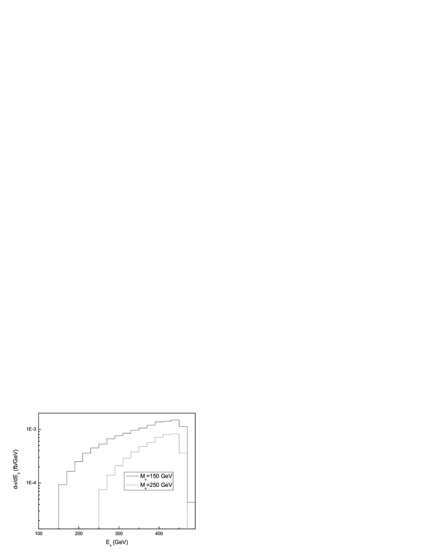
Figure 4: Differential cross sections versus $E_{Z}$ and $E_{\phi^{-}}$ graphs for $\sqrt{s}=1.0TeV$, $f=1000GeV$, $M_{Z_{H}}=2.0TeV$ and two values of $M_{\phi}$. (a) for $Z$ boson, (b) for charged Higgs boson $\phi^{-}$.

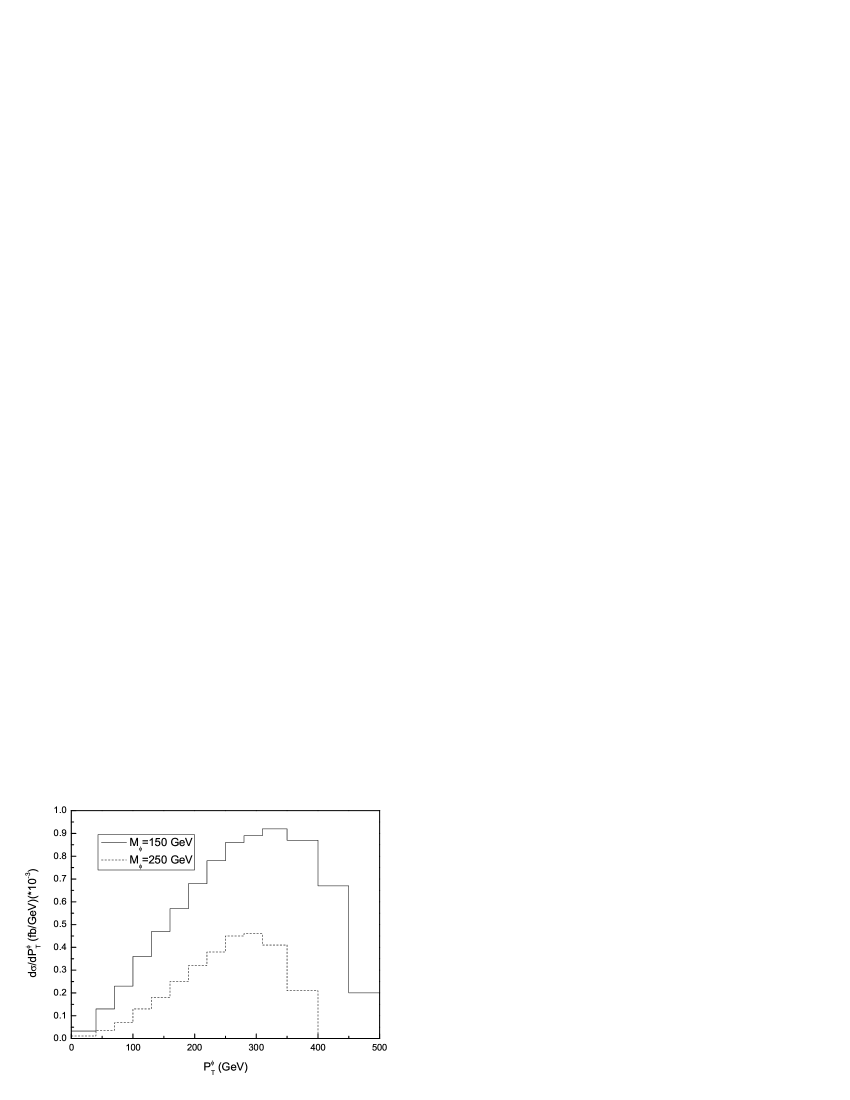
Figure 5: Distributions of the transverse momenta of $Z$ boson and charged Higgs boson $\phi^{-}$ for the $e^{+}e^{-}\rightarrow Z\phi^{+}\phi^{-}$ process with $\sqrt{s}=1.0TeV$ and two values of $M_{\phi}$. (a) for $Z$ boson, (b) for charged Higgs boson $\phi^{-}$.

The distributions of the energy of $Z$ boson and charged Higgs boson $\phi^{-}$ are shown in Fig. 4 for $\sqrt{s}=1.0TeV$ and $M_{\phi}=150GeV$ and $250GeV$, respectively. We can see from the Fig.4(a) that the peak values of differential cross sections are obtained at the order of $10^{-3}\frac{fb}{GeV}$ for low $E_{Z}$ values, $E_{Z}\sim 100GeV$. Meanwhile, the values of $E_{\phi^{-}}$ ranging from $400GeV$ to $450GeV$ make the main contribution to the cross section of $e^{+}e^{-}\rightarrow Z\phi^{+}\phi^{-}$.
In Fig.5, we provide the distributions of transverse momenta of $p_{T}^{Z}$ and $p_{T}^{\phi^{-}}$ with $\sqrt{s}=1.0TeV$ and two values of the charged Higgs bosons mass. From these two figures we can see that, the significant regions of $p_{T}$ for $Z$ boson and charged Higgs boson $\phi^{-}$ are in the regions of $50GeV\sim 100GeV$, and $250GeV\sim 350GeV$, respectively.

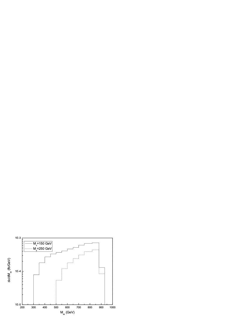
Figure 6: (a) Distributions of the invariant mass of charged Higgs bosons pair with $\sqrt{s}=1.0TeV$ and two values of $M_{\phi}$. (b) Differential cross sections of the cosine of the angle between the produced charged Higgs bosons pair with $\sqrt{s}=1.0TeV$ and two values of $M_{\phi}$.

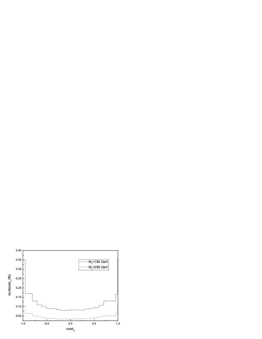
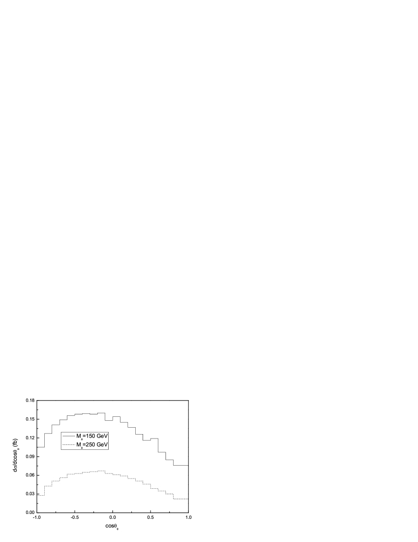
Figure 7: Distributions of the cosine of the $Z$ boson ( charged Higgs boson $\phi^{-}$) production angle with respect to z-axis for the $e^{+}e^{-}\rightarrow Z\phi^{+}\phi^{-}$ process with $\sqrt{s}=1.0TeV$ and two values of $M_{\phi}$. (a) for $\frac{d\sigma}{d\cos\theta_{Z}}$, (b) for $\frac{d\sigma}{d\cos\theta_{\phi^{-}}}$.

The distribution of the charged Higgs bosons pair invariant mass $M_{\phi\phi}$ is shown in Fig. 6(a), and the differential cross section of the cosine of the angle between the produced charged Higgs bosons pair is shown in Fig.6(b) where we take two values of $M_{\phi}$ and $\sqrt{s}=1.0TeV$. We can see from the Fig.6(a) that the relatively large $M_{\phi\phi}$ region (from $700GeV$ to $880GeV$) make the main contribution to the production cross section of $e^{+}e^{-}\rightarrow Z\phi^{+}\phi^{-}$. Fig.6(b) shows the distribution of cosine of the angle between the produced charged Higgs bosons pair. We can see from the figure that the produced charged Higgs boson pair prefer to go out almost back to back, that leads to the $M_{\phi\phi}$ having the tendency to distribution in large value region.
We take the orientation of incoming electron as the z-axis. The $\theta_{Z}$ (or $\theta_{\phi^{-}}$) is defined as the $Z$-boson (or charged Higgs boson $\phi^{-}$) production angle with respect to the z-axis. In Fig.7(a,b) we present the distributions of cosines of the pole angles of $Z$-boson and charged Higgs boson $\phi^{-}$ ($\cos\theta_{Z}$ and $\cos\theta_{\phi^{-}}$) respectively, in conditions of $\sqrt{s}=1.0TeV$ and two values of $M_{\phi}$. From Fig.7(a), it can be seen that the outgoing $Z$-boson is symmetry in the forward and background hemisphere region, while Fig.7(b) demonstrates that the significant regions of $\cos\theta_{\phi^{-}}$ for charged Higgs boson $\phi^{-}$ are rather large.

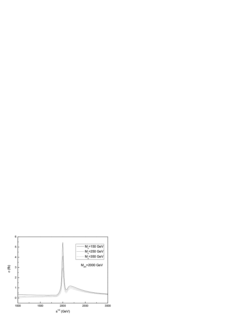
Figure 8: The production cross section $\sigma$ versus $\sqrt{s}$ for $M_{Z_{H}}=1500GeV$ (left), and $M_{Z_{H}}=2000GeV$(right), and three different values of the charged Higgs mass.

To show the influence of c.m. energy on the cross section $\sigma$, in Fig.8, we give the cross section plots as the function of $\sqrt{s}$ with fixed $M_{Z_{H}}$ and three values of the charged Higgs bosons mass $M_{\Phi}$. From Fig.8, we can see that the cross section $\sigma$ resonance emerges when the $Z_{H}$ mass $M_{Z_{H}}$ approaches the c.m. energy $\sqrt{s}$. The resonance values of the $\sigma$ decrease as $M_{Z_{H}}$ increase. For $M_{Z_{H}}=1500GeV$ and $M_{Z_{H}}=1500GeV$ and $2000GeV$, the cross section $\sigma$ can reach $6.9fb$ and $5.5fb$, respectively. Therefor, if we assume the integrated luminosity for the ILC is $500fb^{-1}$, there will be thousands of $Z\phi^{+}\phi^{-}$ signal events generated at the ILC.

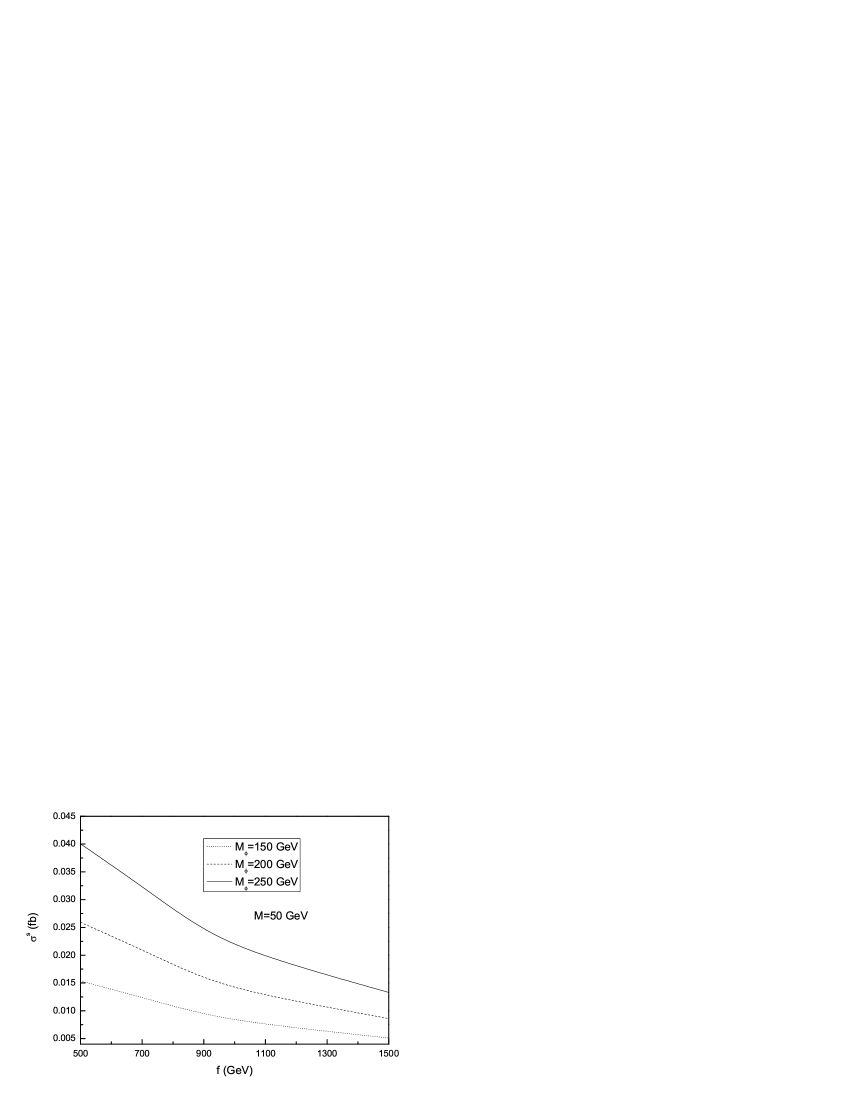
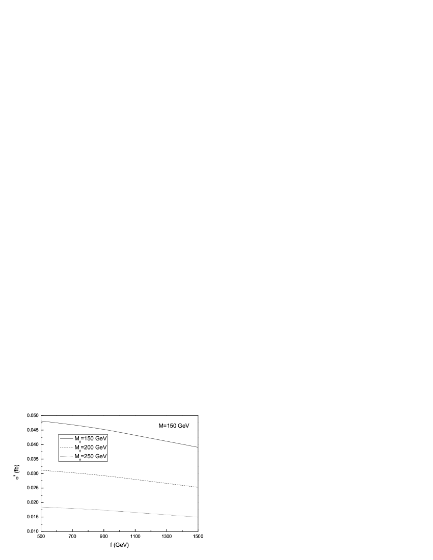
Figure 9: The production rate of the $t\bar{t}b\bar{b}b\bar{b}$ final state as a function of the parameter $f$ for $\sqrt{s}=1.0TeV$, $M=50GeV$ (left), and $M=150GeV$(right), and various values of $M_{\phi}$.

Considering the subsequent decay of $\phi^{+}\rightarrow t\bar{b}$, $t\rightarrow W^{+}b\rightarrow l^{+}\nu b$, the characteristic signal final state of $Z\phi^{+}\phi^{-}$, including four $b$ jets + four charged lepton ($e$ or $\mu$) +missing $E_{T}$ and six jet $q\bar{q}b\bar{b}b\bar{b}$ + two lepton +missing $E_{T}$, which are coming from the $Z$ boson decaying to a charged leptons and $q\bar{q}$, respectively. The $Z$ boson in the final state gives an unambiguous event identification via its leptonic decay. In the case of $Z\rightarrow b\bar{b}$, the production rate of the $t\bar{t}b\bar{b}b\bar{b}$ final state can be easily estimated $\sigma^{s}\approx\sigma\times[Br(Z\rightarrow b\bar{b})\times Br(\phi^{+}\rightarrow t\bar{b})\times Br(\phi^{-}\rightarrow\bar{t}b)]$. The numerical results are shown in Fig.9. One can see from this figure that, with reasonable values of the free parameters of the LRTH model, the production rate can reach $0.04fb$. However, its value decreases quickly as the mass of charged Higgs bosons $M_{\phi}$ increases. The main backgrounds for the $t\bar{t}b\bar{b}b\bar{b}$ final state come from the SM processes $e^{+}e^{-}\rightarrow t\bar{t}hh$, $e^{+}e^{-}\rightarrow t\bar{t}Zh$ and $e^{+}e^{-}\rightarrow t\bar{t}ZZ$ with $Z\rightarrow b\bar{b}$ and $h\rightarrow b\bar{b}$, continuum $t\bar{t}b\bar{b}b\bar{b}$ production. For $\sqrt{s}=1.0TeV$, the total production rate of the $t\bar{t}b\bar{b}b\bar{b}$ backgrounds is estimated to be about $0.01fb$. Thus, it may be possible to extract the signals from the backgrounds in the reasonable parameter spaces in the LRTH model. In addition, the reconstruction of $W$, $t$, and $\phi^{\pm}$ can be used to discriminate the signal from the background. Certainly, detailed confirmation of the observability of the signals generated by the process $e^{+}e^{-}\rightarrow Z\phi^{+}\phi^{-}$ would require Monte-Carlo simulations of the signals and backgrounds, which is beyond the scope of this paper.
IV. The process of $e^{+}e^{-}\rightarrow Z\phi^{0}\phi^{0}$
With the couplings $\phi^{0}\phi^{0}h$, $h\phi^{0}Z_{i}$, and $\phi^{0}\phi^{0}ZZ_{i}$, the processes $e^{+}e^{-}\rightarrow Z\phi^{0}\phi^{0}$ can be induced at tree-level. The Feynman diagrams of these process are shown in Fig.10. The amplitudes of the process $e^{+}e^{-}\rightarrow Z\phi^{0}\phi^{0}$ can be written as:

Figure 10: Feynman diagrams of the process $e^{+}e^{-}\rightarrow Z\phi^{0}\phi^{0}$ in the left-right twin Higgs model.

$$\mathcal{M}_{2}=\mathcal{M}_{a}+\mathcal{M}_{b}+\mathcal{M}_{c}+\mathcal{M}_{d},$$ (24)

with

$$\mathcal{M}_{a} = \sum_{i=2}^{3}\bar{v_{e}}(p_{2})i\gamma_{\mu}(g_{V_{i}}+g_{A_{i}}\gamma_{5})u_{e}(p_{1})\frac{ig^{\mu\nu}}{p_{12}^{2}-M_{i}^{2}+iM_{i}\Gamma_{i}}(iV^{hZ_{i}Z})g_{\nu\alpha}$$ (25)

$$\times\epsilon^{\alpha}(p_{3})\frac{i}{(p_{4}+p_{5})^{2}-M_{h}^{2}}V_{h\phi^{0}\phi^{0}},$$

$$\mathcal{M}_{b} = \sum_{i=2}^{3}\bar{v_{e}}(p_{2})i\gamma_{\mu}(g_{V_{i}}+g_{A_{i}}\gamma_{5})u_{e}(p_{1})\frac{ig^{\mu\nu}}{p_{12}^{2}-M_{i}^{2}+iM_{i}\Gamma_{i}}(iV_{h\phi^{0}Z_{i}})p_{12_{\nu}}$$ (26)

$$\times\frac{i}{(p_{3}+p_{5})^{2}-M_{h}^{2}}(iV_{h\phi^{0}Z})p_{3_{\alpha}}\epsilon^{\alpha}(p_{3}),$$

$$\mathcal{M}_{c} = \sum_{i=2}^{3}\bar{v_{e}}(p_{2})i\gamma_{\mu}(g_{V_{i}}+g_{A_{i}}\gamma_{5})u_{e}(p_{1})\frac{ig^{\mu\nu}}{p_{12}^{2}-M_{i}^{2}+iM_{i}\Gamma_{i}}(iV_{h\phi^{0}Z_{i}})p_{12_{\nu}}$$ (27)

$$\times\frac{i}{(p_{3}+p_{4})^{2}-M_{h}^{2}}(iV_{h\phi^{0}Z})p_{3_{\alpha}}\epsilon^{\alpha}(p_{3}),$$

$$\mathcal{M}_{d} = \sum_{i=2}^{3}\bar{v_{e}}(p_{2})i\gamma_{\mu}(g_{V_{i}}+g_{A_{i}}\gamma_{5})u_{e}(p_{1})\frac{ig^{\mu\nu}}{p_{12}^{2}-M_{i}^{2}+iM_{i}\Gamma_{i}}(iC_{i1}^{\phi^{0}\phi^{0}})g_{\nu\alpha}\epsilon^{\alpha}(p_{3}).$$ (28)

Figure 11: The production cross section $\sigma$ of $e^{+}e^{-}\rightarrow Z\phi^{0}\phi^{0}$ versus $f$ for $\sqrt{s}=0.5TeV$, $M_{Z_{H}}=3.0TeV$ and various values of $M_{\phi^{0}}$.

In the framework of the LRTH model, the mass of the neutral Higgs boson $\phi^{0}$ can be anything below $f$ here we consider another possibility, in which the mass is about $150GeV$[8, 10]. In our numerical estimation, we will assume that the neutral Higgs boson mass $M_{\phi^{0}}$ is in the range of $100GeV-180GeV$.
From the relevant coupling constants in appendix B, we can see that the production cross section of the process $e^{+}e^{-}\rightarrow Z\phi^{0}\phi^{0}$ is very sensitive to the parameter $f$, which is suppressed by the factor of $(v^{2}/2f^{2})$. In this case, we will take the parameter $f$ and the neutral Higgs boson mass $M_{\phi^{0}}$ as the free parameters. The numerical results of the cross section versus the scalar parameter $f$ are shown in Fig.11. We can see that $\sigma$ is sensitive to the parameter $f$ and the mass of the neutral Higgs boson $M_{\phi^{0}}$. For $\sqrt{s}=0.5TeV$, the value of the cross section $\sigma$ are smaller than $1.3\times 10^{-3}fb$ in most of all parameter space preferred by the electroweak precision data, which is really tiny and very difficult to detect in practice.

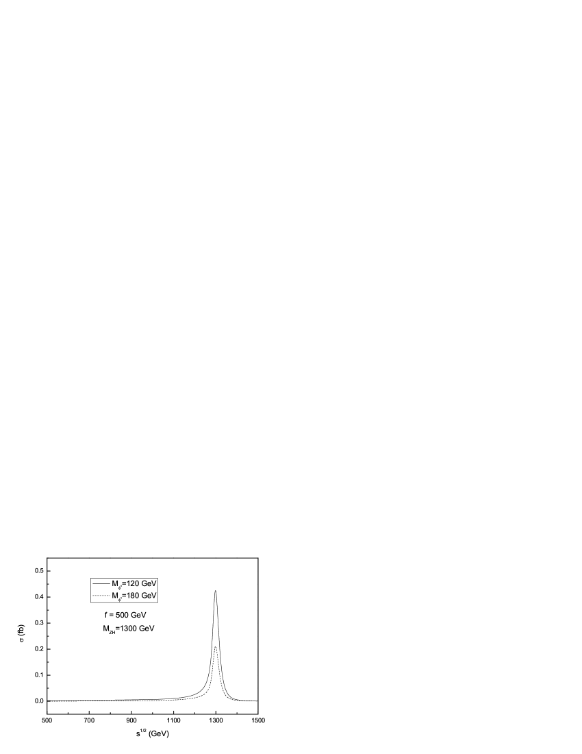
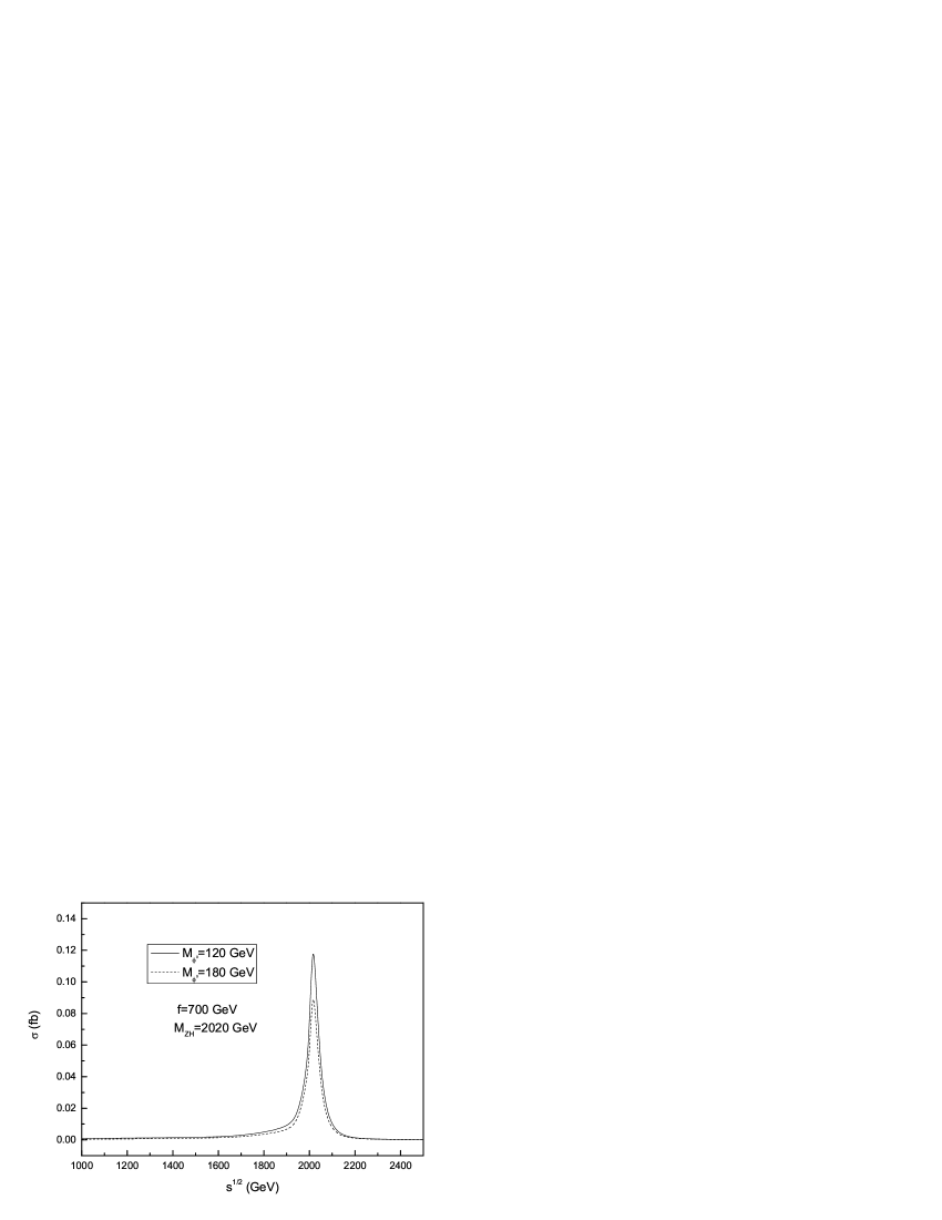
Figure 12: The production cross section $\sigma$ of $e^{+}e^{-}\rightarrow Z\phi^{0}\phi^{0}$ versus $\sqrt{s}$ for $f=500GeV$(left), $f=800GeV$right), and two typical values of $M_{Z_{H}}$.

To see the effects of the c.m. energy $\sqrt{s}$ on the cross section $\sigma$, we plot the $\sigma$ versus $\sqrt{s}$ in Fig.12 for two typical values of the scalar parameter $f$ and $M_{Z_{H}}$. From Fig.12, we can see that the cross section $\sigma$ resonance emerges when the $Z_{H}$ mass $M_{Z_{H}}$ approaches the c.m. energy $\sqrt{s}$. The resonance values of the $\sigma$ are strongly dependent on the $M_{\phi^{0}}$ and the scalar parameter $f$. For $M_{\phi^{0}}=120GeV$ and $f=500GeV$ and $700GeV$, the cross section $\sigma$ can reach $0.5fb$ and $0.14fb$, respectively. Therefor, if we assume the integrated luminosity for the CLIC is $1000fb^{-1}$, there will be tens of up to several hundreds $Z\phi^{0}\phi^{0}$ events to be generated at the CLIC.
Preliminary study in Ref.[13] shows that, for $M_{\phi^{0}}=120GeV$ and $f\leq 700GeV$, the branching ratios $\phi^{0}\rightarrow b\bar{b}$ are larger than $40\%$. The SM Higgs boson $h$ has similar decay features with those of $\phi^{0}$. Therefore, the signatures of $Z\phi^{0}\phi^{0}$ is similar to those of $b\bar{b}hh$, $Zhh$, $ZZZ$, and $ZZh$ at the high energy colliders. For $\sqrt{s}=2.0TeV$, the production cross section of the processes $e^{+}e^{-}\rightarrow b\bar{b}hh$, $e^{+}e^{-}\rightarrow Zhh$, $e^{+}e^{-}\rightarrow ZZh$ and $e^{+}e^{-}\rightarrow ZZZ$ are estimated to be about $0.007fb$, $0.054fb$, $0.14fb$, and $0.45fb$, respectively. The mainly background about six $b$ jets final state has been extensively studied in Ref.[21]. The production rate of this kind of signal is too small to be separated from the large background.
V. Conclusions
Many models of new physics beyond the SM predict the existence of neutral or charged scalar particles. These new particles might produce observable signatures in the current of future high energy experiments different form the case of the SM Higgs boson. Any visible signal from the new scalar particles will be evidence of new physics beyond the SM. Thus, studying the new scalar particles production is very interesting at the ILC.
The Left-right twin Higgs model is a concrete realization of the twin Higgs mechanism, which predicts the existence of three additional Higgs bosons: one neutral Higgs $\phi^{0}$ and a pair of charged Higgs bosons $\phi^{\pm}$. In this paper, we studied the production of a pair of charged and neutral Higgs bosons associated with standard model gauge boson $Z$ at the ILC. From our numerical results, we can obtain the following conclusion: (i) For the process $e^{+}e^{-}\rightarrow Z\phi^{+}\phi^{-}$, for $\sqrt{s}=1000GeV$ and $150GeV\leq M_{\Phi}\leq 400GeV$, the total production cross section is in the range of $0.4\times 10^{-2}fb\sim 0.33fb$. If we assume that the future ILC experiment with $\sqrt{s}$=1.0 TeV has a yearly integrated luminosity of $500fb^{-1}$, then there will be $10^{2}-10^{3}$ signal events generated at the ILC. Furthermore, the $s$-channel resonance effect induced by the $Z_{H}$ gauge boson can significantly enhance the production rate and produce enough signals. The characteristic signal final state of 4$b$ jets + four charged lepton +missing $E_{T}$ might be easily separated from the SM background with a great significance. (ii) For the process $e^{+}e^{-}\rightarrow Z\phi^{0}\phi^{0}$, the value of the cross section $\sigma$ are smaller than $6\times 10^{-3}fb$ in most of all parameter space preferred by the electroweak precision data. However, for $\sqrt{s}\approx M_{Z_{H}}$, the cross section $\sigma$ can be significantly enhanced. Thus, we expect that the future ILC experiments can be seen as an ideal tool to detect the possible signatures of the charged and neutral Higgs bosons predicted by the LRTH model. Even if we can not observe the signals in future ILC experiments, at least, we can obtain the bounds on the free parameters of the LRTH model.

Acknowledgments
We thank Shufang Su for providing the CalcHep Model Code. This work is supported in part by the National Natural Science Foundation of China(Grant No.10775039), and by the Foundation of He nan Educational Committee (Grant No.2009B140003).

Appendix A: The relevant coupling constants in the process $e^{+}e^{-}\rightarrow Z\phi^{+}\phi^{-}$

$i$	vertices	$g_{V_{i}}$	$g_{A_{i}}$
$1$	$e\bar{e}\gamma$	e	0
$2$	$e\bar{e}Z$	$-\frac{e}{2S_{W}C_{W}}[(-\frac{1}{2}+2S_{W}^{2})+\frac{v^{2}}{4(f^{2}+\hat{f}^{2})}\frac{S_{W}^{2}(2C_{W}^{2}-3)}{C_{W}^{4}}]$	$-\frac{e}{2S_{W}C_{W}}[\frac{1}{2}++\frac{v^{2}}{4(f^{2}+\hat{f}^{2})}\frac{S_{W}^{2}(2C_{W}^{2}-1)}{C_{W}^{4}}]$
$3$	$e\bar{e}Z_{H}$	$\frac{e}{4S_{W}C_{W}\sqrt{1-2S_{W}^{2}}}(-1+4S_{W}^{2})$	$\frac{e}{4S_{W}C_{W}\sqrt{1-2S_{W}^{2}}}(2S_{W}^{2}-1)$

  Table 1: The vector and axial vector couplings of $e\bar{e}$ with vector bosons. Feynman rules for $e\bar{e}V_{i}$ vertices are given as $i\gamma_{\mu}(g_{V_{i}}+g_{A_{i}}\gamma_{5})$ [8].

$i/j$	vertices	$iE_{ij}^{\phi^{+}\phi^{-}}Q_{\mu}$
$1/1$	$\phi^{+}\phi^{-}A_{\mu}$	$-ie(p_{1}-p_{2})_{\mu}$
$2/1$	$\phi^{+}\phi^{-}Z_{\mu}$	$i\frac{eS_{W}}{C_{W}}(p_{1}-p_{2})_{\mu}$
$3/1$	$\phi^{+}\phi^{-}Z_{H_{\mu}}$	$-i\frac{e(1-3S_{W}^{2})}{2S_{W}C_{W}\sqrt{1-2S_{W}^{2}}}(p_{1}-p_{2})_{\mu}$

  Table 3: Feynman rules for $\phi^{+}\phi^{-}V_{i}$ vertices. $p_{1}$ and $p_{2}$ refer to the out coming momentum of the first and second particle, respectively. [8].

$hX_{1}X_{2}$	$V_{hX_{1}X_{2}}$	$X_{1}X_{2}h$	$V_{\phi^{+}\phi^{-}h}$
$hZ_{\mu}Z_{\nu}$	$eM_{W}g_{\mu\nu}/(C_{W}^{2}S_{W})$	$\phi^{-}\phi^{+}h$	$x(p_{3}\cdot p_{3}+2p_{1}\cdot p_{2})/(3\sqrt{2}f)$
$hZ_{\mu}Z_{H_{\nu}}$	$e^{2}fxg_{\mu\nu}/(\sqrt{2}C_{W}^{2}\sqrt{1-2S_{W}^{2}})$

  Table 4: Relevant coupling constants of the Higgs boson in Fig. 1(c). $p_{1}$, $p_{2}$ and $p_{3}$ refer to the incoming momentum of the first,second and third particle, respectively. [8].

Appendix B: The relevant coupling constants in the process $e^{+}e^{-}\rightarrow Z\phi^{0}\phi^{0}$

$i/j$	vertices	$iC_{ij}^{\phi^{0}\phi^{0}}g_{\mu\nu}$
$2/1$	$\phi^{0}\phi^{0}Z_{\mu}Z_{\nu}$	$-i\frac{e^{2}x^{2}}{54C_{W}^{2}S_{W}^{2}}g_{\mu\nu}$
$3/1$	$\phi^{0}\phi^{0}Z_{H_{\mu}}Z_{\nu}$	$-i\frac{e^{2}x^{2}}{54C_{W}^{2}\sqrt{1-2S_{W}^{2}}}g_{\mu\nu}$

Table 5: Feynman rules for $\phi^{0}\phi^{0}Z_{i}Z$ vertices [8].

$h\phi^{0}Z_{i}$	$V_{h\phi^{0}Z_{i}}$	$hX_{1}X_{2}$	$V_{h\phi^{0}\phi^{0}}$
$h\phi^{0}Z_{\mu}$	$iexp_{3_{\mu}}/6S_{W}C_{W}$	$h\phi^{0}\phi^{0}$	$\frac{x}{27\sqrt{2}f}(30p_{2}\cdot p_{3}+11p_{1}\cdot p_{1})$
$h\phi^{0}Z_{H_{\mu}}$	$i\frac{ex}{18S_{W}C_{W}\sqrt{1-2S_{W}^{2}}}[(14-17S_{W}^{2})p_{2_{\mu}}-(4-S_{W}^{2})p_{1_{\mu}}]$

  Table 6: Relevant coupling constants of the neutral scalar. $p_{1}$, $p_{2}$ and $p_{3}$ refer to the incoming momentum of the first,second and third particle, respectively. [8].

References

[1]
H. Georgi and A. Pais, Phys. Rev. D10 (1974) 539; Phys. Rev. D12 (1975) 508.
[2]
D. B. Kaplan and H. Georgi, Phys. Lett. B136 (1984) 183;
D. B. Kaplan, H. Georgi and S. Dimopoulos, Phys. Lett. B136 (1984) 187; H. Georgi and D. B. Kaplan, Phys. Lett. B145 (1984) 216.
[3]
N. Arkani-Hamed, A. G. Cohen, and H. Georgi, Phys. Lett. B513 (2001) 232.
[4]
N. Arkani-Hamed, A. G. Cohen, E. Katz, A. E. Nelson, T. Gregoire,
and J. G. Wacker, JHEP0208 (2002) 021; I. Low, W.
Skiba, and D. Smith, Phys. Rev. D66 (2002) 072001; D. E.
Kaplan and M. Schmaltz, JHEP0310 (2003) 039.
[5]
Z. Chacko, H. S. Goh and R. Harnik, Phys. Rev. Lett96
(2006) 231802; Z. Chacko, Y. Nomura, M. Papucci and G. Perez, JHEP0601 (2006) 126.
[6]
Z. Chacko, H. S. Goh and R. Harnik, JHEP0601 (2006)
108.
[7]
A. falkowski, S. Pokorski and M. Schmaltz, Phys. Rev. D74 (2006) 035003.
[8]
H.S. Goh and S. Su, Phys. Rev. D75 (2007) 075010.
[9]
Hock-Seng Goh and C. A. Krenke, Phys. Rev. D 76 (2007)
115018; Phys. Rev. D81 (2010) 055008; A. Abada and I.
Hidalgo, Phys. Rev. D 77 (2008) 113013; E. M. Dolle and
Shufang Su, Phys. Rev. D77 (2008) 075013; Yao-Bei Liu,
Xue-Lei Wang, Hong-Mei Han and Yong-Hua Cao, Commun. Theor.
Phys.49(2008) 977; Yao-Bei Liu and Jie-Fen Shen, Mod.
Phys. Lett. A24 (2009) 143; Chong-Xing Yue, Hui-Di Yang and
Wei Ma, Nucl. Phys. B818 (2009) 1; P. Batra and Z.
Chacko, Phys. Rev. D79 (2009) 095012; Hock-Seng Goh, C.
A. Krenke, Phys. Rev. D81 (2010) 055008; Lei Wang and
Jin Min Yang, JHEP1005 (2010) 024.
[10]
Dong-Won Jung and Jae-Young Lee, hep-ph/0701071.
[11]
Yao-Bei Liu, Xue-Lei Wang, Jun Cao and Hong-Mei Han, Commun.
Theor. Phys.50(2008) 445; Yao-Bei Liu, Lin-Lin Du and Qin
Chang, Mod. Phys. Lett. A24 (2009) 463; Yao-Bei Liu,
Shuai-Wei Wang, Int. J. Mod. Phys. A24 (2009) 4261;
Yao-Bei Liu and Xue-Lei Wang, Europhys. Lett.86, 61002
(2009).
[12]
Yao-Bei Liu, Hong-Mei Han and Xue-Lei Wang, Eur. Phys. J. C53(2008) 615.
[13] Wei Ma, Chong-Xing Yue and Yong-Zhi Wang, Phys. Rev. D 79 (2009) 095010.
[14]
J. Brau (Ed.) et al, By ILC Collaboration, LC Reference Design
Report: ILC Global Design Effort and World Wide Study.,
FERMILA-APC, Aug 2007, arXiv: acc-ph/0712.1950.
[15]
CLIC Physics Working Group (E. Accomando et al.), hep-ph/0412251.
[16]
J. J. Lopez-Villarejo, J. A. M. Vermaseren, arXiv:
0812.3750[hep-ph]; A. Djouadi, V. Driesen, C. Junger, Phys.
Rev. D 54 (1996) 759.
[17]
A. Djouadi, H. E. Haber, P. M. Zerwas, Phys. Lett. B375
(1996) 203; J. L. Feng, T. Moroi, Phys. Rev. D 56 (1997)
5962; H. Grosse, Yi Liao, Phys. Rev. D 64 (2001) 115007;
N. Delerue, K. Fujii, N. Okada, Phys. Rev. D 70 (2004)
091701; Yao-Bei Liu, Lin-Lin Du and Xue-Lei Wang, J. Phys. G
33 (2007) 577; A. Arhrib, R. Benbrik, C. W. Chiang, Phys. Rev. D 77 (2008) 115013; Yao-Bei Liu, Xue-Lei Wang and
Hong-Mei Han, Europhys. Lett.81 (2008) 31001; R. N.
Hodgkinson, D. Lopez-Val, Joan Sola, Phys. Lett. B673
(2009) 47; A. Cagil and M. T. Zeyrek,Phys. Rev. D 80
(2009) 055021; A. Gutierrez-Rodriguez, M. A. Hernandez-Ruiz, O. A.
Sampayo, arXiv:0903.1383 [hep-ph].
[18]
K. Hagiwara, D. Zeppenfeld. Nucl. Phys. B313, (1989)560;
V. Barger, Han Tao, D. Zeppenfeld. Phys. Rev. D41,
(1990)2782.
[19]
A. Pukhov et al., hep-ph/9908288; hep-ph/0412191.
[20]
C. Amsler et al. [Particle Data Group] Phys. Lett. B667
(2008) 1.
[21]
A. Djouadi, et al., Eur. Phys. J. C 10 (1999)27; E.
Coniavitis, A. Ferrari, Phys. Rev. D 75 (2007) 015004;
U. Baur, Phys. Rev. D80 (2009) 013012; Y. Takubo,
arXiv:0901.3598 [hep-ph]; arXiv:0907.0524 [hep-ph].