Ballistic deposition patterns beneath a growing KPZ interface

Abstract

We consider a $(1+1)$ dimensional ballistic deposition process with next-nearest neighbor interaction, which belongs to the KPZ universality class, and introduce for this discrete model a variational formulation similar to that for the randomly forced continuous Burgers equation. This allows to identify the characteristic structures in the bulk of a growing aggregate (“clusters” and “crevices”) with minimizers and shocks in the Burgers turbulence, and to introduce a new kind of equipped Airy process for ballistic growth. We dub it the “hairy Airy process” and investigate its statistics numerically. We also identify scaling laws that characterize the ballistic deposition patterns in the bulk: the law of “thinning” of the forest of clusters with increasing height, the law of transversal fluctuations of cluster boundaries, and the size distribution of clusters. The corresponding critical exponents are determined exactly based on the analogy with the Burgers turbulence and simple scaling considerations.

I Introduction

Over the past few decades, the problem of growth of aggregates by sequential stochastic deposition developed into one of the most extensively studied topics in statistical physics zhang . Much effort has been put into theoretical, numerical, and experimental investigation of the resulting patterns. Several theoretical models have been proposed, including the famous Kardar–Parisi–Zhang (KPZ) KPZ and Edwards–Wilkinson (EW) EW models, the Restricted Solid-on-Solid (RSOS) rsos and Eden eden models, the models of Molecular Beam Epitaxy (MBE) MBE , Polynuclear Growth (PNG) M ; PS ; PNG ; BR ; J , and several ramifications of the Ballistic Deposition (BD) model Mand ; MRSB ; KM ; BMW . Within the latter, in the simplest setting, one assumes that elementary units (“particles”) follow ballistic trajectories in space and adhere sequentially to a growing aggregate (“heap”). Despite its extremely transparent geometric formulation, the problem of stochastic growth still is one of the most puzzling problems in statistical mechanics.

The available theoretical analysis of stochastic deposition focuses almost exclusively on the enveloping surface $h(x,t)$, involving a statistical study of its height distribution and the corresponding scaling exponents. Here we quote just a few prominent results. The essential scaling relations characterizing the growing aggregate are

$$\langle\mathop{\mathrm{Var}}\tilde{h}(x,t)\rangle^{1/2} \sim t^{1/3},$$

$$\langle\tilde{h}(x,t)\,\tilde{h}(x+t^{2/3}l,t)\rangle-\langle\tilde{h}\rangle^{2} \sim t^{2/3}F(l).$$

Here $\tilde{h}(x,t)=h(x,t)-ct$, $c=\lim_{t\to\infty}t^{-1}h(x,t)$ is an average speed of growth, and $F(l)$ is a rescaled correlation function. The exponents $1/3$ and $2/3$ were determined already in KPZ for the KPZ model and then observed in a variety of other growth models. Then in Refs BDJ ; PS it was realized that the distribution of a rescaled PNG height $t^{-1/3}(h(0,t)-2t)$ converges as $t\to\infty$ to the Tracy–Widom distribution TW for the Gaussian unitary ensemble (GUE), which appears in the theory of random matrices. Moreover, the full rescaled PNG surface $t^{-1/3}(h(xt^{2/3},t)-2t)+x^{2}$ converges to a version of the Airy stochastic process $Airy_{2}(x)$ PNG whose one-point distributions are precisely Tracy–Widom. Distribution of maximal heights of the $(1+1)$ dimensional Edwards–Wilkinson and KPZ interfaces has been determined exactly in Ref. SC .

It should be pointed out that the BD model considered below involves the point-to-line last-passage percolation while PNG corresponds to the point-to-point setting J . Correspondingly the limit processes are different: it is $Airy_{1}$ for the point-to-line and $Airy_{2}$ for the point-to-point. Note also that the one-point distribution for the $Airy_{1}$ process is given by the Gaussian orthogonal ensemble (GOE) distribution rather than the GUE distribution, which corresponds to $Airy_{2}$.

Since a similar convergence to Airy processes is observed in other growth models such as TASEP sasam , it is becoming customary to speak of “the KPZ universality class” whenever such limit behavior is present. For example, a KPZ scaling has been shown in Refs scaling1 ; scaling2 ; scaling3 for the BD model in the thermodynamic limit.

Much less is known, however, about the structure of BD patterns beneath the enveloping surface. Here is just one puzzle: analytic arguments Vershik.A:2000a predict that the expected density $\rho_{\rm surf}$ of local surface maxima in a $(1+1)$ dimensional ballistically growing heap is $\rho_{\rm surf}=1/3$, whereas extensive numerical simulations show that the mean bulk density, $\rho_{\rm bulk}$, of the $(1+1)$ dimensional heap is about $0.25\approx 1/4$. To date there is no satisfactory quantitative explanation of this mismatch.

The statistics of the growing heap are determined by its striking internal structure, revealed in numerical simulations as well as in the recent experimental analysis of electrochemically formed silver branched patterns silver . This structure consists of a “forest” formed by tree–like clusters of different size, which are separated by a dual network of tree–like channels or “crevices” (Fig. 1).

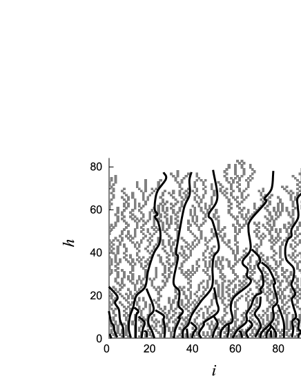
Figure 1: Snapshot of a heap obtained by ballistic deposition of $N=2000$ particles in a periodic box of size $L=100$ with next-nearest-neighbor interactions. Black lines trace the channels (“crevices”) between adjacent clusters.

As the heap grows, clusters randomly collect particles and thus spread and isolate their neighbors from the “rainfall” of incident particles, suffocating their growth. Consequently the number of clusters present at height $h$ in a growing aggregate is a decreasing function of $h$. We remark that this “suffocation” mechanism, as well as the growth patterns in the BD model, bear certain similarity to those observed in diffusion limited aggregation in a hard–core lattice gas on a zero–temperature boundary oshanin3 , although the two models belong to different universality classes and their quantitative behaviors are in no direct correspondence.

In the present work we undertake investigation of clusters and crevices based on a novel systematic analogy with turbulent structures in randomly forced Hamilton–Jacobi equations. This allows us to conclude that BD belongs to a large group of models within the KPZ universality class, such as PNG model, TASEP, and others. It turns out that BD like other models mentioned above admits a variational formulation. Moreover the analogy with Hamilton–Jacobi dynamics enables us to suggest a novel concept of equipped Airy process, a buildup on top of classical Airy processes which also takes into account the geometrical structure of the optimal paths (maximizers of the action, see Section III). The random field of optimal paths arises naturally in the context of stochastically forced Burgers equation EKMS ; khanin_bec .

In a recent experimental work silver the size distribution $P(m)$ of frozen structures formed by electrochemically grown silver branching patterns has been analyzed. The authors found that the probability $P(m)$ to have a cluster of size $m$ exhibits scale invariance, i.e. $P(m)\sim m^{\tau}$, with a critical exponent $\tau=1.37\pm 0.04$. In our work we compute this exponent analytically ($\tau=7/5$) and show that the scaling behavior conjectured in silver actually holds as well as two other power laws governing the “thinning” of the forest of clusters with increasing height and the transversal fluctuations of the cluster boundaries.

The paper is organized as follows. In Section II we specify the model and define its main structural features. Section III contains an analysis of the structural similarity of BD patterns to “minimizers” and “shocks” in the Burgers turbulence khanin_bec , based on the common variational formulation of the two models. In Section IV we discuss the KPZ scaling in the BD model and introduce the notion of an equipped Airy process. Building on these developments, in Section V we compute the main scaling exponents of the BD model. Section VI contains concluding remarks and outlook for future work.

II The model and basic definitions

II.1 The NNN ballistic deposition model

A standard $(1+1)$ dimensional BD model with next-nearest-neighbor (NNN) interactions can be formulated as follows (see also Refs scaling1 ; scaling2 ; scaling3 ). Consider a box divided into $L$ columns of unit width each, enumerated with index $i$ ($i=1,2,\dots,L$). For simplicity we assume the periodic boundary conditions, so that the leftmost and the rightmost columns are neighbors, and identify the index value $0$ with $L$.

At the initial time $t=0$ the system is empty. Then, at each time step $t=1,2,\dots,t_{\rm max}$, an elementary unit (“particle”) of height $\ell$ and width $1$ is deposited at a column $i(t)$ chosen randomly with uniform distribution.

Define

$$\eta_{i}(t)=\begin{cases}1,&i=i(t),\\ 0,&i\neq i(t).\end{cases}$$ (1a)

As shown in Fig. 1, particles deposited in adjacent columns interact in such a way that they can only touch each other at corners or at top and bottom, but never along their vertical sides. Let the height of column $$i t-1 h_{i}(t-1)$$ at time be . Upon adding a particle it changes according to

$$h_{i}(t)=\begin{cases}\max\{h_{i-1}(t-1),h_{i}(t-1),\text{\hbox to0.0pt{$h_{i+1}(t-1)\}+\ell,$\hss}}\\ {}&\eta_{i}(t)=1,\\[8.61108pt] \mathstrut\qquad h_{i}(t-1),&\eta_{i}(t)=0.\end{cases}$$ (1b)

This dynamics is supplemented with the initial condition $h_{i}(0)\equiv 0$ for all $1\leq i\leq L$. Eqs (1a), (1b) completely describe updating rules for the NNN discrete ballistic deposition.

We will use Eq. (1b) represented in a different form. Define the “thin” and “thick” discrete “$\delta$–functions”

$$L_{k,i}^{0}=\begin{cases}\infty&|k-i|>0,\\ 0&|k-i|=0,\end{cases}\quad L_{k,i}^{1}=\begin{cases}\infty&|k-i|>1,\\ 0&|k-i|\leq 1\end{cases}.$$ (2)

Consider first the trivial dynamics described by the equation $h_{i}(t)=h_{i}(t-1)$. It can be rewritten as $h_{i}(t)=\max\limits_{k}\,[h_{k}(t-1)-L_{k,i}^{0}]$: indeed, $\max\limits_{k\neq i}\,[h_{k}(t-1)-\infty]\equiv-\infty$ and therefore $h_{i}(t)=\max\,\{h_{i}(t-1),-\infty\}=h_{i}(t-1)$. It is now clear that the stochastic equation (1b) can be recast in the form

$$h_{i}(t)=\max_{k}\,[h_{k}(t-1)-L_{k,i}^{\eta_{i}(t)}]+\ell\eta_{i}(t).$$ (3)

This dynamics should be compared with the commonly used discrete equation with “additive noise” describing the $(1+1)$ dimensional polynuclear growth PNG , which in our notation takes the form

$$\tilde{h}_{i}(t)=\max_{k}\,[\tilde{h}_{k}(t-1)-L_{k,i}^{1}]+\ell\eta_{i}(t).1`$$ (4)

According to Eq. (3), the height $h_{i}$ remains unchanged (quenched) if nothing is deposited to column $i$ at time $t$. On the contrary, in Eq.(4) the height $\tilde{h}_{i}$ relaxes spontaneously even in the absence of deposition to column $i$ at time $t$ because $\tilde{h}_{i}(t)$ is defined to be the maximum of the triple $\{\tilde{h}_{i-1}(t-1),\tilde{h}_{i}(t-1),\tilde{h}_{i+1}(t-1)\}$. Note that process described by Eq.(3) is sometimes referred to as “dynamics with multiplicative noise.”

II.2 Clusters, crevices, and scaling exponents in the growing heap

Let us now take a closer look at Fig. 1. We say that two particles in a heap are connected if they touch one another at corners or if one is situated directly on the top of the other.

It often happens that the upper particle is connected simultaneously to two lower particles. For reasons that will become clear shortly, it is better to avoid these “one-on-two” configurations. The model is therefore slightly augmented: one assumes in Eqs (1b) and (3) that

$$\ell=\ell(t)=1+10^{-10}\xi(t),$$ (5)

where $\xi(t)$ are independent normal random variables. It is clear, and well supported by numerical experiments, that this modification removes the possibility of “one-on-two” configurations while preserving, within the limits of statistical errors, statistical characteristics of the heap for $\ell\equiv 1$. Alternatively one might resolve “one-on-two” configurations for $\xi=0$ by simply disconnecting the upper particle from one of its two lower neighbors at random. Either way, elimination of one-on-two configurations allow us to define a unique “path” corresponding to every particle, namely a backward directed chain of connected particles going from a given particle to the bottom level of the heap.

Consider all connected paths originating from the topmost particles. These paths can merge. We define the backbone of a cluster as the connected set of such paths, i.e., the union of all paths that end up at the same bottom level particle. It is easy to see that the bottom level particles are split into two classes: those that are reached by the paths originated at the top of the heap and those that are not. Obviously the first class gets smaller as $t$ increases. For every particle from this class define cluster as the collection of all paths ending up at this particle. The difference between a backbone and a cluster is that clusters contain paths not necessarily originating from the top level particles.

We say that a pair of two top level particles occupying adjacent columns defines a shock, which is located between them, if they belong to two different clusters. The channel of white space between two neighboring clusters is called a crevice. Clearly every crevice is associated with a shock at the top, and the connected paths from top particles defining the shock form the left and right boundary of a crevice. Connecting shocks at adjacent time moments, we get curves that branch forward in time and play a role dual to that of backbones. These curves are sketched in Fig. 1 in black.

It is clear from Fig. 1 that many channels that are initially present at bottom of the bulk then merge at some height, blocking the growth of the clusters situated in between. Thus crevices have tree-like structure just as clusters, but contrary to clusters they merge upward. This causes the number of percolating clusters and crevices to decrease as a function of $h$. In the thermodynamic limit this behavior is characterized by the following three scaling exponents whose values are identified in Section V.

The thinning exponent $\alpha$ characterizes the expected number $\langle c(h)\rangle$ of percolating crevices (or, equivalently, percolating clusters) at height $h$:

$$\langle c(h)\rangle\sim h^{-\alpha}$$ (6)

The wander exponent $\beta$ characterizes the expected mean square displacement (in the units of $L$) of the boundary of percolating cluster between the bottom of the bulk and a specified height $h$:

$$\langle\Delta x^{2}(h)\rangle\sim h^{\beta}$$ (7)

The mass exponent $\tau$ characterizes the mass distribution of clusters:

$$P(m)\sim m^{-\tau},$$ (8)

where $P(m)$ is the proportion of clusters of mass $m$ in the ensemble.

III Ballistic deposition and Burgers turbulence

III.1 Variational formulation of the BD

The discrete equation

$$h_{i}(t)=\max_{k}\,[h_{k}(t-1)-L_{k,i}(t)]+\ell\eta_{i}(t),$$ (9)

whose particular cases for specific choices of $L_{k,i}(t)$ are the BD model (3) and the discrete PNG model (4), admits a natural variational formulation.

Fix some initial condition $h_{i}(0)$ and consider the discrete “variational” problem of finding a trajectory $(\gamma(0),\gamma(1),\dots,\gamma(t))$ that satisfies the “boundary condition” $\gamma(t)=i$ and maximizes the discrete “action”

$$\mathcal{A}_{0}^{t}(\gamma)=h_{\gamma(0)}(0)-\sum_{1\leq s\leq t}[L_{\gamma(s-1),\gamma(s)}(s)-\ell\eta_{\gamma(s)}(s)].$$ (10)

The function in the square brackets plays a role of a discrete “Lagrangian” of the system. The problem bears an obvious resemblance to the zero temperature limit of the free energy of a statistical system, expressed as the sum over configurations $\gamma$:

$$\lim_{T\to 0}T\ln(e^{\frac{1}{T}A_{1}}+\dots+e^{\frac{1}{T}A_{N}})\to\max\{A_{1},\dots,A_{N}\}$$

Another obvious connection is with mechanics, where the dynamical trajectory can be found by optimizing the corresponding action (in our case, at variance with the usual convention, the action is maximized).

Action maximization in Eq. (10) is related to solving Eq. (9) as follows. To be specific, consider the BD growth (3), where particles are added to the system as “dropping events” $(i(s),s)$ in $(1+1)$ dimensional discrete space-time. Maximization of the action $\mathcal{A}_{0}^{t}$ in (10) amounts to finding a trajectory that terminates at $(i,t)$ and passes through a maximal number of dropping events under the following constraint: the trajectory stays constant, $\gamma(s)=\gamma(s-1)$, unless $\gamma(s-1)=i(s)\pm 1$, i.e., there is a dropping event in adjacent column. In the latter case the trajectory may (but does not necessarily have to) jump to $i(s)$ at time step $s$. Note that for the PNG model (4) this constraint is relaxed: a trajectory may jump at all times, but only to adjacent columns. Otherwise the two models are structurally similar, and the rest of the argument in this subsection applies to both.

The lack of a strict obligation to pass through an adjacent dropping event allows to “collect” dropping events more efficiently: it is easy to construct trajectories for which it is more profitable, from the point of view of maximizing the number of dropping events, to skip some isolated dropping events in order not to be driven away from a later series of several adjacent dropping events.

Direct maximization of the action (10) is a difficult problem because the solution depends on the whole future history of dropping events. Observe however that for all $1\leq j\leq L$, $1\leq s\leq t$ the height function $h_{j}(s)$ gives the maximal number of dropping events available for a trajectory coming to the point $(j,s)$, and this fact can be exploited to construct a maximizing trajectory in reverse time.

Consider again the BD case where $L_{k,j}(s)=L_{k,j}^{\eta_{j}(s)}$. Then the maximizing trajectory passing through an arbitrary $(i,t)$ can be reconstructed by setting $\gamma(t)=i$ and solving recursively

$$\gamma(s-1)=\arg\max_{k}\,[h_{k}(s-1)-L^{\eta_{\gamma(s)}(s)}_{k,\gamma(s)}]+\ell\eta_{\gamma(s)}(s)$$ (11)

for $s=t,t-1,\dots,1$. Here $\arg\max_{k}$ is the standard notation for the value of $k$ that provides maximum to the expression in the r.h.s. of (11).

The algorithmic implementation of the above goes as follows. Solve first Eq. (9) “upstairs” starting from given initial conditions and obtain the set of values $h_{1}(s),h_{2}(s),\dots,h_{L}(s)$ for all $0\leq s\leq t$. Then choose a specific point, say $(i,t)$, and restore the path to this point going “downstairs,” i.e., back in time, by solving Eq. (11) step by step. This procedure defines a trajectory maximizing the action $\mathcal{A}_{0}^{t}$ in Eq. (10). This class of algorithms is known in the optimization theory as dynamic programming, and Eq. (9) is called the Bellman equation (see, e.g., the classical book bellman ).

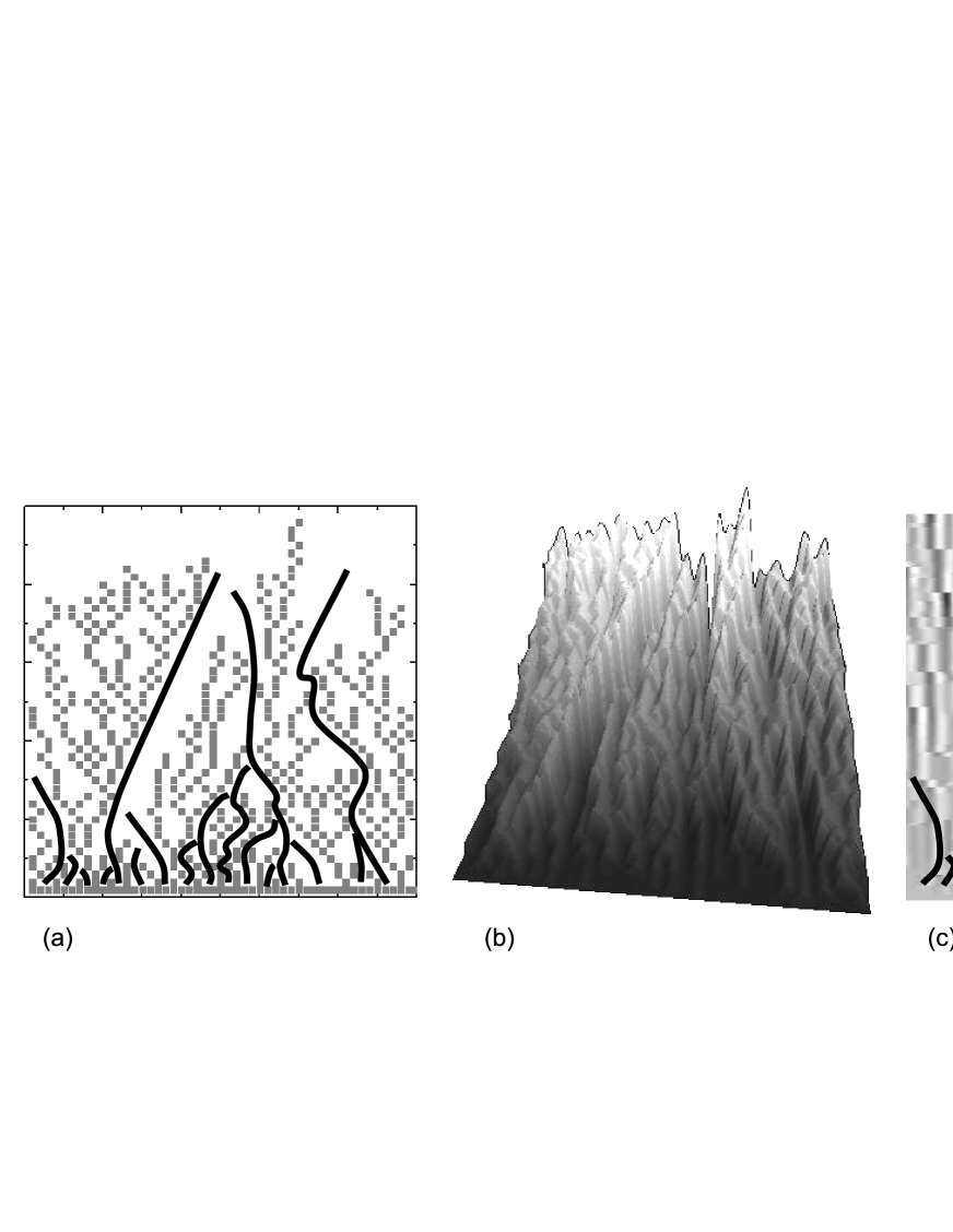
Figure 2: (a) Heap growing by sequential deposition with highlighted crevices; (b) the growing heap in the $(2+1)$ dimensional spacetime; (c) density plot of 2nd local difference (discrete analog of 2nd derivative) of the height, which highlights the discontinuities corresponding to shocks. Panes (a) and (c) represent front and top views, respectively, of the three-dimensional structure in pane (b).

III.2 BD heaps and the Burgers turbulence

It turns out that there is a far-reaching analogy between the BD deposition model and phenomenology of “shocks” and “minimizers” for the Burgers or Hamilton–Jacobi equation with random forcing (see, e.g., khanin_bec ). We first recall the latter.

Consider the inviscid Burgers equation

$$\partial_{t}u+u\partial_{x}u=-\partial_{x}\eta(x,t),$$

where $\eta(x,t)$ is the forcing potential. The substitution $u=\partial_{x}h$ transforms this equation into

$$\partial_{t}h+(\partial_{x}h)^{2}/2+\eta(x,t)=0.$$

More generally, one can consider the Hamilton-Jacobi equation

$$\partial_{t}h+H(\partial_{x}h)+\eta(x,t)=0,$$ (12)

where $H(p)$ is a convex function representing the kinetic energy. Using the Legendre transform representation $H(p)=\max_{v}[pv-L(v)]$, one can write

$$\partial_{t}h+v\,\partial_{x}h-L(v)+\eta(x,t)\leq 0$$

with equality only for $\partial_{x}h=L^{\prime}(v)$, i.e., $v=H^{\prime}(\partial_{x}h)$. Hence along any trajectory $\gamma(t)$ the rate of change of $h$ is bounded by the Lagrangian

$$\frac{d}{dt}h(\gamma,t)\leq L(\dot{\gamma})-\eta(\gamma,t)$$

(here $\dot{\gamma}=d\gamma/dt$), which implies for any $\gamma$ passing through $x$ at time $t$ that

$$h(x,t)\leq\mathcal{A}_{0}^{t}[\gamma]=h(\gamma(0),0)+\int_{0}^{t}[L(\dot{\gamma})-\eta(\gamma,s)]\,ds$$ (13)

with equality only for minimizers of the action, which must satisfy the equation

$$\dot{\gamma}(t)\equiv H^{\prime}(\partial_{x}h(\gamma,t)).$$ (14)

The Hamilton–Jacobi equation (12) is thus intimately connected with the variational problem of minimizing the action (13), just as the Bellman equation (9) arises in maximization of the discrete “action” (10). Note in particular the similar structure of the action (the difference in sign results in maximization replacing minimization in the discrete case). Moreover, a known solution $h$ to (12) allows to reconstruct minimizing trajectories using (14), much as (11) generates maximizing trajectories in the discrete problem.

It is therefore natural to consider the discrete maximizing trajectories defined in the previous subsection as analogs of continuous minimizers. There is one apparent difference: continuous minimizers never cross, while discrete maximizing paths merge and form tree-like structures. However continuous minimizers have a tendency to approach each other with exponential rate in reverse time due to hyperbolicity, and in the discrete case the same hyperbolicity manifests itself in the exponentially decreasing probability for two adjacent maximizers to stay separate as time runs backwards.

We are now in position to establish the relation between discrete maximizers and connected paths defined within the heap in Section II. Lift the maximizing trajectories to the $(i,t,h)$ space by setting $h=\mathcal{A}_{0}^{t}(\gamma)$ for a maximizer $\gamma$ such that $\gamma(t)=i$. Then connected paths are given by the projection of these “lifted” maximizers to the $(x,h)$ plane (see Fig. 2). In other words, the intervals of time between successive dropping events along a maximizer are collapsed into unit steps in $h$. Correspondingly the transversal fluctuations of maximizers as a function of time are transformed to transversal fluctuations of connected path as a function of height $h$.

The analogy between continuous minimizers and discrete maximizers extends to shocks. In the Burgers turbulence it typically happens that two or more minimizing trajectories, which start at different initial locations, pass through same point $x$ at time $t$, so that the map from $(x,t)$ to the initial location is discontinuous (see, e.g., khanin_bec ). These discontinuities are called shocks; in spacetime they form continuous shock curves. This definition is obviously parallel to the definition of shocks given in the BD setting in Section II (and has inspired the latter).

IV From BD patterns to Airy processes

IV.1 Basics of classical KPZ scaling

Recall first the basics of classical KPZ scaling related to $Airy_{1}$ process, which is closest to our setting. The scheme described below is due to Sasamoto sasam .

Consider a directed random walk on a $(1+1)$ dimensional lattice. Suppose that the space-time lattice is equipped by a random potential with independent values $\eta_{i}(s)$ at each point $(i,s)$. Then for every $i$ one can consider the maximum of an action over all random walk paths of length $t$ terminating at that point, i.e., define

$$a_{i}(t)=\max_{\gamma\colon\gamma(t)=i}\sum_{1\leq s\leq t}\eta_{\gamma(s)}(s).$$

where $L_{k,i}$ is a “kinetic” part of the action that ensures a certain control of how far the trajectory $\gamma$ can jump over unit time steps. It is easy to see that $t^{-1}\,a_{i}(t)\to c$ at $t\to\infty$, where $c$ is some nonrandom constant independent of $i$. We now consider the rescaled process

$$A_{t}(x)=\frac{1}{\beta t^{1/3}}\,(a_{\alpha t^{2/3}x}(t)-ct).$$ (15)

The main statement is that $A_{t}(x)$ converges as $t\to\infty$ to a universal spatially homogeneous limit process called $Airy_{1}(x)$. Universality here means that whenever one optimizes in a disordered medium the action of a path from a point that varies over a line to a parallel line separated from the first one by distance $t$ (“point-to-line last-passage percolation”), the process corresponding to the optimal action converges as $t\to\infty$ to the $Airy_{1}$ process.

Note that spatial homogeneity of $Airy_{1}(x)$ immediately follows from the construction. Of course one has to ensure convergence by subtracting the mean value of order $t$, normalizing the difference by $t^{1/3}$ and rescaling the starting point by $t^{2/3}$. The constants $\alpha$ and $\beta$ in (15) are nonuniversal and should be chosen properly to ensure convergence to the standard Airy process. A similarly rescaled “point-to-point” percolation results in the $Airy_{2}$ process.

IV.2 The Airy process for BD pattern

As we have shown in Section III the height function in the BD process can be viewed as given by maximization procedure for random paths in random potential. The only difference with the classical picture just described is related to the rarity of the deposition events. In other words, in order to achieve the displacement of order 1 in space direction one needs time of order $L$. This explains why time has to be rescaled.

The most natural way to do this is through a local stochastic change of time variable. Namely we collapse the time between two deposition events to $1$. This is exactly the transformation from (lifted) maximizers to connected paths presented in Section III. It is therefore no surprise that the $Airy_{1}$ process can be obtained from the BD height function:

$$\lim_{t\to\infty}\frac{1}{\beta(t/L)^{1/3}}(h_{\alpha(t/L)^{2/3}x}(t)-t/L)=Airy_{1}(x).$$ (16)

This formula simply indicates that the appropriately rescaled height function in BD is the visualization of the process which converges in the thermodynamic limit to the Airy process.

IV.3 The “hairy Airy” process

The $Airy_{1}$ process carries only part of the information about the system: it is oblivious to the maximizing trajectory associated to the (rescaled) point $(x,t)$. It is therefore natural to consider the limit

$$\left(\frac{a_{\alpha t^{2/3}x}(t)-ct}{\beta t^{1/3}},\ \frac{\gamma_{\alpha t^{2/3}x,t}(ts)}{\alpha t^{2/3}}\right)\\ \xrightarrow[t\to\infty]{}(Airy_{1}(x),\Gamma_{x}(s)),$$ (17)

where $\gamma_{i,t}$ is the maximizing trajectory that passes through $i$ at time $t$ and $\Gamma_{x}(s)$ is a continuous path defined over $[0,1]$ such that $\Gamma_{x}(1)=x$. We call this limit the equipped Airy process.

As just before, in the BD setting we collapse time intervals between adjacent deposition events to unit steps and get particle paths instead of maximizing trajectories in formula (17) above. Applying transversal rescaling $\alpha(t/L)^{2/3}x$ and height rescaling $\beta(t/L)^{1/3}$ as in (16), we get a realization of equipped Airy process from the rescaled BD heap. This process describes the joint distribution of fluctuations of the height function and transversal displacements of cluster boundaries in the spatially homogeneous BD process.

In other words, the rescaled height function for the BD model alone is a realization of the $Airy_{1}$ process, while the rescaled height function together with the rescaled forest of maximizers corresponds to a realization of the equipped Airy process. The distinctive geometric features of this joint process suggests the name “hairy Airy process,” cf. Fig. 3a.

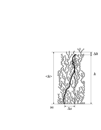
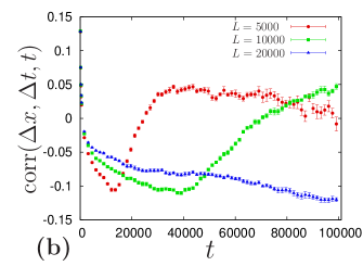
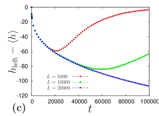
Figure 3: (Color online) a) Correlation between the height of cluster’s boundary and the displacement of the corresponding connected path; b) the corresponding correlation coefficient; c) the averaged difference between the height of cluster’s right boundary and the mean height of the BD growing interface.

We demonstrate the existence of correlations in the joint distribution for the hairy Airy process by computing numerically the joint distribution of the height fluctuation $\Delta h$ at the top of a shock and the corresponding displacement $\Delta x$ of the cluster boundary. To be precise, we compute the correlation coefficient between the fluctuations of the displacement $\Delta x$ of the right boundary of a cluster (or equivalently a backbone) and the height fluctuation $\Delta h$ at the top right point of the same cluster, see Fig. 3a. For convenience we explicitly recall here the standard definition of the correlation coefficient $\mathrm{corr}\{a,b\}$ between two random variables $a$ and $b$:

$$\mathrm{corr}\{a,b\}=\frac{\langle(a-\langle a\rangle)\,(b-\langle b\rangle)}{\sqrt{\langle(a-\langle a\rangle)^{2}\rangle\,\langle(b-\langle b\rangle)^{2}\rangle}}.$$ (18)

Let the top right particle of some cluster be located at time $t$ in column $j$. Let $h_{j}(t)$ be its height and $\langle h(t)\rangle$ the mean height of the whole surface at time $t$. Denote furthermore $h_{j}(t)-\langle h(t)\rangle$ by $\Delta h_{j}(t)$ and the displacement of the right boundary of the same cluster at time $t$, measured from the position of this boundary at $t=0$, by $\Delta x_{j}(t)$. We fix a time $t$, collect for each cluster the joint information $(\Delta h_{j}(t),\Delta x_{j}(t))$, and perform averaging over all clusters. Behavior of the corresponding time-dependent correlation coefficient $\mathrm{corr}\{\Delta h,\Delta x\}$, where the angle brackets correspond to averaging over the sample, is shown in Fig. 3b for different time values.

Strong correlations between the vertical and horizontal displacements of cluster boundaries are clearly seen in the data. The negative sign of these correlations is due to the fact that the height of the top right particle in a typical cluster is smaller than the averaged height of the growing BD interface. This observation is supported by Fig. 3c, where the averaged difference between the height of the cluster right boundary and the averaged height of the interface is plotted against time. Clearly this difference is always negative and tends to $0$ from below as $t\to\infty$. One may speculate that growth of the left- and ritghmost connected paths in a cluster is slower due to screening between neighboring clusters.

In order to better understand the influence of clusters on the morphological structure of the growing BD surface, we also compute the joint distribution of height fluctuations in two columns separated by distance $\delta=3$ in lattice units, as shown in Fig. 4a. Two different situations are distinguished: i) two test column belong to the same cluster (configuration $A$), and ii) two test columns belong to different clusters, i.e., are separated by a shock (configuration $B$).

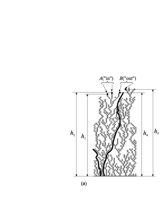
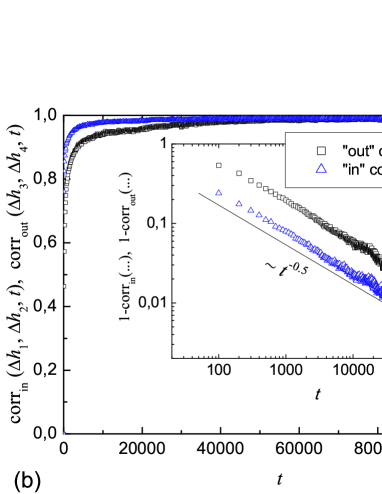
Figure 4: (Color online) a) Correlation between the heights inside the cluster (“in”) and separated by a shock (“out”); b) the corresponding correlation coefficients.

Computing the correlation coefficient $\mathrm{corr}\{\Delta h_{k},\Delta h_{m}\}$ according to (18), we see that correlations between $\Delta h_{1}$ and $\Delta h_{2}$ inside a cluster are stronger than those across a shock between different clusters.

V Scaling analysis of BD patterns

V.1 “Thinning” of clusters and wandering of their boundaries

Relying on the connection between shocks and boundaries of clusters, we can directly transfer the scaling arguments of statistics of shocks developed in khanin_bec to the scaling analysis of a growing BD heap and determine the values of the scaling exponents $\alpha$ and $\beta$ in the dependencies $c(h)\sim h^{-\alpha}$ and $\Delta x^{2}(h)\sim h^{\beta}$ defined correspondingly in Eqs (6) and (7). Recall that $c(h)$ is the averaged number of clusters percolating to height $h$ and $\Delta x^{2}(h)$ is the mean square displacement of a cluster boundary at height $h$.

Denote by $d(t)$ the horizontal size of a cluster at time $t$. At $t=0$ the cluster has zero size, i.e., $d(0)=0$. In what follows we shall use the obvious fact that the growth time $t$ in the sequential deposition process is proportional to the average height $h$ of the growing heap and, consequently, to the cluster height — see, for example, Fig. 2b.

The typical value of $d(h)$ can be obtained by scaling considerations. Namely, growth of $d(h)$ is determined by two additive effects. On the one hand, there is a “driving force” promoting the “smearing” of the cluster due to the velocity fluctuations. For BD this effect can be estimated as follows. Consider clusters with size of order $d$. Under the uniform random “rainfall” of deposited particles, one cluster can randomly screen part of its neighbors, and increase its own “spot.” Since different clusters are correlated weakly, it is natural to conjecture that the typical scale of fluctuations of cluster sizes is of order of $\sqrt{d}$. Thus the rate $v$ of cluster “smearing” due to these fluctuations is $v\sim d/\sqrt{d}\sim d^{-1/2}$. Speaking more carefully, the above means that the average growth rate of the cluster of size $d$ is

$$v=\frac{1}{d}\sum_{k\leq j\leq k+d}(h_{j+1}-h_{j}),$$

where $k$ and $k+d$ are the left and the right boundaries of some cluster. The increments of $h_{j}$ are uncorrelated for the uniform ballistic “rain” and $\langle h_{j+1}-h_{j}\rangle=0$. It is therefore natural to expect that $v\sim d^{-1/2}$ as conjectured.

On the other hand, there is “smearing” of clusters due to the random deposition of new particles near the cluster boundary. This process can be interpreted as “diffusion” of the boundary. Over time $t$ this diffusion leads to the smearing of the cluster’s horizontal size on typical scale of order of $\sqrt{t}$.

The typical size of a growing cluster at time $t$ is determined by additive contributions of these two effects:

$$d(t)\simeq tv+t^{1/2}=\frac{t}{\sqrt{d(t)}}+t^{1/2}$$ (19)

The dominant contribution to $d(t)$ comes from the first term, which is consistent with the physical intuition. Hence,

$$d(t)\sim t^{2/3}$$ (20)

Since $t\sim h$, we immediately come to the conclusion that $d(h)\sim h^{2/3}$. (This estimate is a direct paraphrase of the arguments provided in khanin_bec for scaling analysis of statistics of shocks in the $(1+1)$ dimensional Burgers equation with random forcing).

The density $c(h)$ of independent clusters surviving up to the height $h$ is inversely proportional to the cluster size, $c(h)\sim[d(h)]^{-1}$. Thus,

$$c(h)\sim h^{-2/3},$$ (21)

which gives $\alpha=2/3$.

Furthermore, the typical horizontal mean square displacement $\langle\Delta x^{2}(h)\rangle$ of a cluster boundary at height $h$ can be estimated simply as

$$\langle\Delta x^{2}(h)\rangle=d^{2}(h)\sim h^{4/3},$$ (22)

which gives $\beta=4/3$.

V.2 Mass distribution of clusters

This Section contains the scaling analysis of the probability $P(m)\sim m^{-\tau}$ to find a cluster of mass $m$ in a large aggregate. To begin with, note that the number of particles, i.e., the “mass” $m(h)$ of a cluster percolating to height $h$ can be obtained integrating the horizontal size, $d(h)$, of cluster at a given height:

$$m(h)\sim\int_{0}^{h}(h^{\prime})^{\alpha}\,\mathrm{d}h^{\prime}\sim h^{\alpha+1}.$$ (23)

From (21) we know that the cumulative probability of clusters surviving until height $h$ is of the order of $h^{-\alpha}$. This implies that the probability density of clusters at height $h$ scales as $h^{-(\alpha+1)}\,\mathrm{d}h$. In order to calculate mass distribution, we change variables from $h$ to $m$, take into account that $\mathrm{d}m\sim h^{\alpha}\,\mathrm{d}h$, or $\mathrm{d}h\sim h^{-\alpha}\,\mathrm{d}m=m^{-\alpha/(\alpha+1)}\,\mathrm{d}m$, and get

$$\begin{array}[]{rcl}P(m)&\sim&m^{-\tau}\,\mathrm{d}m\sim h^{-(\alpha+1)}\,\mathrm{d}h\sim m^{-1}\,m^{-\alpha/(\alpha+1)}\,\mathrm{d}m\vskip 6.0pt plus 2.0pt minus 2.0pt\\ &=&m^{-(2\alpha+1)/(\alpha+1)}\,\mathrm{d}m.\end{array}$$ (24)

For $\alpha=2/3$ we get $\tau=7/5$. The exponent $\tau=7/5$ is well supported by our own numerical simulations shown in Fig. 5, and, as mentioned in Introduction, it has been found in independent laboratory experiments on cluster formation in quasi-two-dimensional electrochemically formed silver branching structures silver .

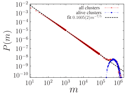
Figure 5: The probability $P(m)$ to find in a large system a cluster of mass $m$.

One can say that he clusters are ranked (ordered) according to their masses and $m$ is the corresponding rank. Thus Eq. (24) has similarity with the Zipf’s law that appears in many areas of science ranging from word statistics in linguistics zipf to nuclear multifragmentation ma ; campi where clusters have power-law distribution in sizes (masses, charges etc.).

VI Conclusion

In this paper we analyze the internal structure of the heap formed in the course of standard homogeneous ballistic deposition with next–nearest–neighboring (NNN) interactions in a box. We have paid the most attention to the statistics of clusters and the channels (crevices) separating them. We have demonstrated that the BD process can be naturally described in terms of “dynamic programming” language associated with the so-called Bellman equation. The “dynamic programming” point of view allows systematic translation of the study of clusters and crevices in the NNN ballistic deposition into the language of maximizers and shocks in discrete equations of the Burgers or Hamilton–Jacobi type. This is the key point of our work. A detailed examination of the corresponding continuous limit will be the subject of a forthcoming publication.

In particular, the results of the work khanin_bec concerning the statistics of shocks in $(1+1)$ dimensional Burgers turbulence with random forcing allow the direct interpretation for statistics of cluster’s boundaries (crevices) of growing heap. This connection between shocks and crevices has permitted us to compute the scaling exponents $\alpha$ ($\alpha=2/3$) in the dependence $\langle c(h)\rangle\sim h^{-\alpha}$, where $\langle c(h)\rangle$ is the average number of clusters, surviving up to height $h$ and $\beta$ ($\beta=4/3$) for the mean square displacement $\langle\Delta x^{2}(h)\rangle\sim h^{\beta}$ of crevices as a function of the height $h$ of the heap.

We have also extended the scaling analysis to the computation of the critical exponent $\tau$ ($\tau=7/5$) of the mass distribution of clusters, $P(m)\sim m^{-\tau}$, where $P(m)$ is the probability density of clusters of mass $m$ (see Fig. 5 for comparison of numerical simulation with scaling dependence (24)). The exponent $\tau$ coincides with the one found in real experiments on cluster formation in quasi–two dimensional electrochemically formed silver branching structures silver .

The investigation of the morphological structure of surface of the growing heap splitted in clusters, has lead us to the definition of a new “equipped” Airy process for BD, named the “hairy Airy process.” In our preliminary investigation we have analyzed numerically its two-point correlation function and have shown the existence of essential correlations between the fluctuations of the displacement $\Delta x$ of the cluster’s left boundary and the height’s fluctuation $\Delta h$ in the top point of the same cluster’s left boundary location, see Fig. 3a.

We believe that the described connection between crevices and shocks could be a useful tool for deeper understanding of both topics, NNN ballistic deposition and Burgers turbulence. For NNN ballistic growth we could apply the machinery developed in turbulence, while for turbulence we could use NNN ballistic deposition for straightforward visualization of some complex chaotic behavior.

Let us end up by noting that many important and puzzling questions concerning the growth of the heap have not been touched in this paper. For instance, we have not discussed the question mentioned in the Introduction: why the bulk density of the heap does not coincide with the density of local maxima of the growing surface. Our guess is that the discrepancy between these densities, $\rho_{\rm bulk}$ and $\rho_{\rm surf}$ is due to the presence of crevices in the heap. Another example remaining almost without the attention deals with the consideration of aging in the growing heap. The investigation of the correlation between two heights inside a cluster and separated by the crevice considered in Fig. 4 gives some hint about the aging of the heap, however we have not considered the correlation between two heights separated by the crevice of finite depth.

- (1) T. Halpin–Healy, and Y.-C. Zhang, Physics Reports 254, 215 (1995)
- (2) M. Kardar, G. Parisi, and Y.-C. Zhang, Phys. Rev. Lett. 56, 889 (1986)
- (3) S.F. Edwards and D.R. Wilkinson, Proc. Roy. Soc. London A 381, 17 (1982)
- (4) J.M. Kim and J. M. Kosterlitz, Phys. Rev. Lett. 62, 2289 (1989)
- (5) F. Family and T. Vicsek, J. Phys. A: Math. Gen. 18, L75 (1985)
- (6) M.A. Herman and H. Sitter, Molecular Beam Epitaxy: Fundamentals and Current, (Springer: Berlin, 1996)
- (7) P. Meakin, Fractals, Scaling, and Growth Far From Equilibrium, (Cambridge University Press: Cambridge, 1998)
- (8) M. Prähofer and H. Spohn, Phys. Rev. Lett. 84, 4882 (2000)
- (9) M. Prähofer, H. Spohn, J. Stat. Phys. 108, 1071 (2002)
- (10) J. Baik and E.M. Rains, J. Stat. Phys. 100, 523 2000
- (11) K. Johansson, Comm. Math. Phys. 242, 277 (2003)
- (12) B.B. Mandelbrot, The Fractal Geometry of Nature, (Freeman, New York, 1982)
- (13) P. Meakin, P. Ramanlal, L. M. Sander, and R. C. Ball, Phys. Rev. A 34, 5091 (1986)
- (14) J. Krug and P. Meakin, Phys. Rev. A 40, 2064 (1989)
- (15) D. Blomker, S. Maier-Paape, and T. Wanner, Interfaces and Free Boundaries 3, 465 (2001)
- (16) J. Baik, P. Deift, and K. Johansson, J. Amer. Math. Soc. 12, 1189 (1999)
- (17) S.N. Majumdar and A. Comtet, Phys. Rev. Lett. 92, 225501 (2004)
- (18) C.A. Tracy and H. Widom, Commun. Math. Phys. 159, 151 (1994)
- (19) G. Costanza, Phys. Rev. E 55, 6501 (1997)
- (20) F.D.A. Aarao Reis, Phys. Rev. E 63, 056116 (2001)
- (21) E. Katzav and M. Schwartz, Phys. Rev. E 70, 061608 (2004)
- (22) A.M. Vershik, S.K. Nechaev, and R. Bikbov, Comm. Math. Phys. 212, 469 (2000)
- (23) C. M. Horowitz, M. A. Pasquale, E. V. Albano, and A. J. Arvia, Phys. Rev. B 70, 033406 (2004)
- (24) S. F. Burlatsky, G. Oshanin, and M. Elyashevich, Physics Letters A, 151, 538 (1990)
- (25) W. E, K. Khanin, A. Mazel, and Ya. G. Sinai, Ann. of Math. 151, 877 (2000)
- (26) J. Bec and K. Khanin, Phys. Rep., 447, 1 (2007)
- (27) R.E. Bellman, Dynamic Programming (Dover Publications: 2003)
- (28) T. Sasamoto, J. Phys. A 38, L549 (2005)
- (29) G.K. Zipf, Human Behavior and the Principle of Least Effort, (Addisson–Wesley Press: Cambridge, MA, 1949).
- (30) A. Dabrowska et al., Acta Phys. Pol. B 35, 2109 (2004); Y. G. Ma et al. (NIMROD Collaboration), Phys. Rev. C 71, 054606 (2005).
- (31) X. Campi and H. Krivine, Phys. Rev. C 72, 057602 (2005)