Semi-Analytic Stellar Structure in Scalar-Tensor Gravity

M.W. Horbatsch1 and C.P. Burgess1,2
1 Dept. of Physics & Astronomy, McMaster University
  1280 Main St. W, Hamilton, Ontario, Canada, L8S 4L8.

2 Perimeter Institute for Theoretical Physics
  31 Caroline St. N, Waterloo, Ontario, Canada N2L 2Y5.
Abstract:

Precision tests of gravity can be used to constrain the properties of hypothetical very light scalar fields, but these tests depend crucially on how macroscopic astrophysical objects couple to the new scalar field. We study the equations of stellar structure using scalar-tensor gravity, with the goal of seeing how stellar properties depend on assumptions made about the scalar coupling at a microscopic level. In order to make the study relatively easy for different assumptions about microscopic couplings, we develop quasi-analytic approximate methods for solving the stellar-structure equations rather than simply integrating them numerically. (The approximation involved assumes the dimensionless scalar coupling at the stellar center is weak, and we compare our results with numerical integration in order to establish its domain of validity.) We illustrate these methods by applying them to Brans-Dicke scalars, and their generalization in which the scalar-matter coupling slowly runs – or ‘walks’ – as a function of the scalar field: a(ϕ)as+bsϕsimilar-to-or-equals𝑎italic-ϕsubscript𝑎𝑠subscript𝑏𝑠italic-ϕa(\phi)\simeq a_{s}+b_{s}\phi. (Such couplings can arise in extra-dimensional applications, for instance.) The four observable parameters that characterize the fields external to a spherically symmetric star are the stellar radius, R𝑅R, mass, M𝑀M, scalar ‘charge’, Q𝑄Q, and the scalar’s asymptotic value, ϕsubscriptitalic-ϕ\phi_{\infty}. These are subject to two relations because of the matching to the interior solution, generalizing the usual mass-radius, M(R)𝑀𝑅M(R), relation of General Relativity. Since ϕsubscriptitalic-ϕ\phi_{\infty} is common to different stars in a given region (such as a binary pulsar), all quantities can be computed locally in terms of the stellar masses. We identify how these relations depend on the microscopic scalar couplings, agreeing with earlier workers when comparisons are possible. Explicit analytical solutions are obtained for the instructive toy model of constant-density stars, whose properties we compare to more realistic equations of state for neutron star models.

1 Introduction

One way in which candidate quantum theories of gravity can differ from one another is the spectrum of bosons they predict at very low energies. Such fields, if they exist and are sufficiently light, can mediate long-range forces that can observably compete with gravity.

Scalar-tensor theories of gravity are among those that can arise in this way, with light scalar fields in addition to the usual metric tensor [1, 2, 3, 4, 5, 6]. A variety of scalars commonly arise in fundamental theories, although it is very unusual for them to be light enough to mediate forces over macroscopic distances. They are rarely this light because quantum corrections famously tend to give scalars masses, even if they would have been massless at the purely classical level. But in some circumstances symmetries can protect against masses, such as if the scalar is a pseudo-Goldstone boson [7] for a spontaneously broken approximate symmetry, or part of the low-energy limit of an extra-dimensional model [8].

A good deal of effort has been invested in comparing the predictions of scalar-tensor theories with observations in various astrophysical systems [9, 10, 11, 12, 13, 14, 15, 16, 17], in order to improve the constraints on their existence (or to discover their presence). Binary pulsars are particularly useful for this purpose, since the precision of their timing allows accurate measurements of the relativistic gravitational effects that are generated by the strong gravitational fields present.

Central to these tests is an understanding of how the stellar properties depend on the microscopic couplings of the scalar field to matter. Yet these stellar properties can sometimes be remarkable in scalar-tensor theories in the presence of relativistic sources. In particular a phenomenon called spontaneous scalarization can occur, in which the star above a critical baryonic mass can locally support a scalar field even if the scalar-matter coupling vanishes asymptotically far from the star [18]. This allows scalar-tensor gravity to deviate strongly from General Relativity (GR) near the star while still passing weak-field solar system tests.

Since different fundamental theories predict scalars with different microscopic couplings, it is useful to be able to survey how stellar properties depend on these couplings. For this reason in this paper we re-examine the equilibrium conditions in a star in scalar-tensor models as a function of scalar couplings. In particular we do so working as far as possible within analytic approximation schemes, since these more easily allow the results to be varied for different kinds of scalar properties. We find semi-analytic progress is possible using a weak-coupling approximation for the scalar field near the stellar center. By comparing with numerical integrations of the equations of stellar structure we find the domain of validity of these approximations, which allow us to understand stellar properties fairly well.

As a preliminary to studying the relativistic limit in more detail, we apply our analysis to the special case of an incompressible stellar fluid, for which the energy density is approximately constant. (This can be done consistent with conservation laws only if the pressure is not also regarded as being a function of the energy density.) To leading order in the weak-coupling expansion, the profiles of physical variables of constant-density stars can be described in closed form in terms of elementary functions, dilogarithms, and Heun functions.

Although not physically realistic, solutions with this equation of state can give insight into general features of relativistic stars, in particular near the maximum mass that can be supported by gravitational forces. (For GR the maximum mass found under the assumption of constant density gives an upper bound on the maximum mass that would be found with more realistic equations of state [19].) We compare the predictions of constant density in scalar-tensor theory with those of several representative equations of states for neutron stars.

The rest of the paper is organized as follows. In §2 we define the scalar-tensor theories of interest, and in particular the parameters describing the couplings of the light scalar to ordinary matter. Following much of the literature we specialize to the case where the scalar-matter couplings are only weakly dependent on the scalar fields themselves — what we call quasi-Brans/Dicke (qBD) models — as well as the constraints on their couplings that are inferred from solar system tests of gravity. §3 then derives the equations describing hydrostatic equilibrium for static and spherically-symmetric stars in scalar-tensor gravity, as well as the matching formulae that relate the interior and exterior geometries. Some of those general properties that can be extracted without solving them explicitly are also discussed, such as whether the pressure need be monotonic; the kinds of relations they imply amongst quantities visible to exterior observers; and the non-relativistic limit. Next, §4 provides a discussion of the perturbative solutions to these equations in the weak-coupling limit, in both the relativistic and non-relativistic cases. The important distinction between perturbations in the strength of the coupling measured at the stellar center, vs its strength at infinity, first arises in this section. Finally, in section §5 the perturbed equations are solved explicitly to leading nontrivial order for the special case of incompressible stars, with the results compared to more realistic equations of state for neutron star models.

2 Single-field scalar-tensor models

We start by defining the field equations of the scalar-tensor systems of interest.

2.1 Action and field equations

We consider a single light scalar field, and choose its action to be given by111Conventions: we use metric signature (+++)(-+++) and Weinberg’s curvature conventions [20] (differing from MTW [21] only by an overall sign for the Riemann tensor). Units are chosen with =c=1Planck-constant-over-2-pi𝑐1\hbar=c=1.

S=116πGd4xggμν(μν+2μϕνϕ)+Sm[ψ,g~μν],𝑆116𝜋𝐺superscriptd4𝑥𝑔superscript𝑔𝜇𝜈subscript𝜇𝜈2subscript𝜇italic-ϕsubscript𝜈italic-ϕsubscript𝑆m𝜓subscript~𝑔𝜇𝜈S=-\frac{1}{16\pi G}\int{\hbox{d}}^{4}x\sqrt{-g}\;g^{\mu\nu}\bigl{(}\mathcal{R}_{\mu\nu}+2\,\partial_{\mu}\phi\partial_{\nu}\phi\bigr{)}+S_{\rm{m}}[\psi,\tilde{g}_{\mu\nu}]\,, (1)

where a Weyl re-scaling is performed to go to the Einstein frame (which eliminates any ϕitalic-ϕ\phi-dependence from the Einstein-Hilbert term) and the scalar field is redefined to ensure its kinetic term is minimal (with a conventional factor of 2). Here G𝐺G is the Einstein-frame gravitational constant, gμνsubscript𝑔𝜇𝜈g_{\mu\nu}, is the Einstein-frame metric whose Ricci tensor is μνsubscript𝜇𝜈\mathcal{R}_{\mu\nu}, and Smsubscript𝑆mS_{\rm m} denotes the ‘matter’ action, involving all other observed fields (collectively denoted here by ψ𝜓\psi).

There are two physical choices made in writing this action, beyond the choice of using only a single scalar field.

  • We assume the absence of a scalar potential, which we assume is small enough to be negligible for the astrophysical applications of interest. This would necessarily be true if the scalar is relevant to cosmology, but is also the feature that quantum contributions make most difficult to achieve in realistic models (unless there is an approximate symmetry, like shifts ϕϕ+citalic-ϕitalic-ϕ𝑐\phi\to\phi+c, for constant c𝑐c).

  • We assume the matter action, Smsubscript𝑆mS_{\rm m}, only depends on ϕitalic-ϕ\phi and gμνsubscript𝑔𝜇𝜈g_{\mu\nu} through the one ‘Jordan-frame’ combination g~μν=A2(ϕ)gμνsubscript~𝑔𝜇𝜈superscript𝐴2italic-ϕsubscript𝑔𝜇𝜈\tilde{g}_{\mu\nu}=A^{2}(\phi)g_{\mu\nu}, where the conformal factor A(ϕ)𝐴italic-ϕA(\phi) is a function whose form would be specified within any particular fundamental theory. This kind of coupling actually arises in specific models (such as if ϕitalic-ϕ\phi arises as the breathing mode for the geometry of extra dimensions), and has the attractive feature that it naturally evades many of the strongest observational constraints on violations of the equivalence principle.

The field equations obtained by varying (1) are

μν+2μϕνϕ+8πG(Tμν12Tgμν)subscript𝜇𝜈2subscript𝜇italic-ϕsubscript𝜈italic-ϕ8𝜋𝐺subscript𝑇𝜇𝜈12𝑇subscript𝑔𝜇𝜈\displaystyle\mathcal{R}_{\mu\nu}+2\partial_{\mu}\phi\partial_{\nu}\phi+8\pi G\left(T_{\mu\nu}-\frac{1}{2}Tg_{\mu\nu}\right) =\displaystyle= 00\displaystyle 0 (2)
ϕ+4πGa(ϕ)Titalic-ϕ4𝜋𝐺𝑎italic-ϕ𝑇\displaystyle\Box\phi+4\pi Ga(\phi)T =\displaystyle= 0,0\displaystyle 0\,, (3)

where =gμνμνsuperscript𝑔𝜇𝜈subscript𝜇subscript𝜈\Box=g^{\mu\nu}\nabla_{\mu}\nabla_{\nu} is the d’Alembertian operator built using the Levi-Civita connection of gμνsubscript𝑔𝜇𝜈g_{\mu\nu}, while

Tμν=2gδSmδgμνsuperscript𝑇𝜇𝜈2𝑔𝛿subscript𝑆m𝛿subscript𝑔𝜇𝜈T^{\mu\nu}=-\frac{2}{\sqrt{-g}}\frac{\delta S_{\rm m}}{\delta g_{\mu\nu}} (4)

is the Einstein-frame energy-momentum tensor, T=gμνTμν𝑇superscript𝑔𝜇𝜈subscript𝑇𝜇𝜈T=g^{\mu\nu}T_{\mu\nu} is its trace, and a(ϕ)=A(ϕ)/A(ϕ)𝑎italic-ϕsuperscript𝐴italic-ϕ𝐴italic-ϕa(\phi)=A^{\prime}(\phi)/A(\phi) defines the scalar-matter coupling function in terms of the function A(ϕ)𝐴italic-ϕA(\phi).

2.2 Observational constraints

Because it is g~μνsubscript~𝑔𝜇𝜈\tilde{g}_{\mu\nu} that appears in the matter action, it is the geodesic of this Jordan-frame metric along which the trajectories of matter particles tend to move (in the absence of other forces). Upon taking the post-Newtonian limit of the Jordan-frame metric g~μνsubscript~𝑔𝜇𝜈\tilde{g}_{\mu\nu}, one finds that the effective Jordan-frame gravitational constant, measured in asymptotic Einstein-frame units,222These are units in which the Einstein-frame metric is asymptotically Minkowski: diag(1,1,1,1)1111(-1,1,1,1). If one instead uses units in which the Jordan-frame metric is asymptotically Minkowski, then G~=GA2(ϕ)[1+a2(ϕ)]~𝐺𝐺superscript𝐴2subscriptitalic-ϕdelimited-[]1superscript𝑎2subscriptitalic-ϕ\widetilde{G}=GA^{2}(\phi_{\infty})[1+a^{2}(\phi_{\infty})]. is

G~=G[1+a2(ϕ)],~𝐺𝐺delimited-[]1superscript𝑎2subscriptitalic-ϕ\widetilde{G}=G\Bigl{[}1+a^{2}(\phi_{\infty})\Bigr{]}\,, (5)

and that the Jordan-frame parameterized post-Newtonian quantities whose values differ from those of GR are

β~=1+a2(ϕ)b(ϕ)2[1+a2(ϕ)]2,γ~=12a2(ϕ)1+a2(ϕ),formulae-sequence~𝛽1superscript𝑎2subscriptitalic-ϕ𝑏subscriptitalic-ϕ2superscriptdelimited-[]1superscript𝑎2subscriptitalic-ϕ2~𝛾12superscript𝑎2subscriptitalic-ϕ1superscript𝑎2subscriptitalic-ϕ\tilde{\beta}=1+\frac{a^{2}(\phi_{\infty})b(\phi_{\infty})}{2[1+a^{2}(\phi_{\infty})]^{2}}\,,\qquad\tilde{\gamma}=1-\frac{2a^{2}(\phi_{\infty})}{1+a^{2}(\phi_{\infty})}\,, (6)

where ϕsubscriptitalic-ϕ\phi_{\infty} is the asymptotic value of the scalar field far from the source and b(ϕ)=da(ϕ)/dϕ𝑏italic-ϕd𝑎italic-ϕditalic-ϕb(\phi)={\hbox{d}}a(\phi)/{\hbox{d}}\phi [2].

Constraints on these PPN parameters from solar system observations provide the best bounds on the model, with |γ~1|<2.3×10⁵~𝛾12.3superscript105|\tilde{\gamma}-1|<2.3\times 10^{-5} inferred from Cassini tracking, and |β~1|<2.3×10⁴~𝛽12.3superscript104|\tilde{\beta}-1|<2.3\times 10^{-4} from lunar laser ranging [9]. This corresponds to the coupling bounds

a2(ϕSS)<1.2105anda2(ϕSS)|b(ϕSS)|<4.6104,formulae-sequencesuperscript𝑎2superscriptsubscriptitalic-ϕ𝑆𝑆1.2superscript105andsuperscript𝑎2superscriptsubscriptitalic-ϕ𝑆𝑆𝑏superscriptsubscriptitalic-ϕ𝑆𝑆4.6superscript104a^{2}(\phi_{\infty}^{SS})<1.2\cdot 10^{-5}\,\quad\hbox{and}\quad a^{2}(\phi_{\infty}^{SS})|b(\phi_{\infty}^{SS})|<4.6\cdot 10^{-4}\,, (7)

where ϕSSsuperscriptsubscriptitalic-ϕ𝑆𝑆\phi_{\infty}^{SS} denotes the asymptotic value of ϕitalic-ϕ\phi as one leaves the solar system.

2.3 (Quasi) Brans/Dicke scalars

The simplest scalar-tensor theory is Brans-Dicke theory [22], for which a(ϕ)=as𝑎italic-ϕsubscript𝑎𝑠a(\phi)=a_{s} is constant. In this case – see eq. (7) – solar system tests constrain as<3.5103subscript𝑎𝑠3.5superscript103a_{s}<3.5\cdot 10^{-3}, and so all of the predictions of Brans-Dicke theory are very close to those of GR.

The next-simplest theory, which we call quasi-Brans/Dicke (qBD) theory, allows a(ϕ)𝑎italic-ϕa(\phi) to vary slowly with ϕitalic-ϕ\phi [23]:

A(ϕ)=exp(asϕ+12bsϕ2),a(ϕ)=as+bsϕ.formulae-sequence𝐴italic-ϕsubscript𝑎𝑠italic-ϕ12subscript𝑏𝑠superscriptitalic-ϕ2𝑎italic-ϕsubscript𝑎𝑠subscript𝑏𝑠italic-ϕA(\phi)=\exp(a_{s}\phi+\textstyle{\frac{1}{2}}\,b_{s}\phi^{2})\,,\qquad a(\phi)=a_{s}+b_{s}\phi\,. (8)

This introduces a variety of new phenomena because it makes the strength of the scalar-matter couplings depend on ϕitalic-ϕ\phi, and so allows them to vary with position and time [24, 25]. This means that couplings in exotic environments (like stellar interiors) could be stronger than naïvely expected without running into conflict with the strong solar-system bounds mentioned above (this is similar in spirit to, but different in detail from, evading these bounds through matter-dependent scalar self-couplings [26, 27, 28]). Assuming ϕitalic-ϕ\phi is defined such that ϕ0italic-ϕ0\phi\to 0 asymptotically far from the Sun, eqs. (7) show that the strong bound on assubscript𝑎𝑠a_{s} implies that solar system bounds do not strongly constrain bssubscript𝑏𝑠b_{s}.

The constraints on bssubscript𝑏𝑠b_{s} are comparatively weak, and the best come from studies of binary pulsars [29, 30, 31]. The precise timing measurements that are possible for binary pulsars allow their orbits to be accurately measured over long periods of time, and comparing measurements with the predictions of the qBD model leads to the constraint bs5greater-than-or-equivalent-tosubscript𝑏𝑠5b_{s}\gtrsim-5 [10, 11, 12, 13]. Measurements of the redshift of spectral lines from neutron stars leads to a weaker constraint bs9greater-than-or-equivalent-tosubscript𝑏𝑠9b_{s}\gtrsim-9 [14]. The main uncertainties in these bounds come from the poor understanding of the nuclear equation of state appropriate for neutron star interiors.

Observations disfavor negative bssubscript𝑏𝑠b_{s} because for bs<4<subscript𝑏𝑠4b_{s}\mathrel{\raise 1.29167pt\hbox{$<$\kern-8.50006pt\lower 4.30554pt\hbox{$\sim$}}}-4, compact objects like neutron stars exhibit a phenomenon called spontaneous scalarization [18]. For sufficiently dense objects, whose precise threshold density depends on bssubscript𝑏𝑠b_{s} and the nuclear equation of state, it is possible for the star to support a nonzero scalar field even though the scalar coupling vanishes asymptotically far from the star: a(ϕ)=0𝑎subscriptitalic-ϕ0a(\phi_{\infty})=0. Furthermore it is known that when scalarization takes place it is the stable solution to the field equations [32, 1]. Scalarized neutron stars tend to be disfavored by binary pulsar observations because scalarization significantly changes the dynamics and radiation generated by a neutron star.

Collapse processes involving scalarized neutron stars have been investigated by a number of authors [33], who found that the waveform of the emitted gravitational radiation depends strongly on bssubscript𝑏𝑠b_{s}. Moreover, scalar-tensor gravity allows monopole and dipole radiation, which are forbidden in GR. Thus, future measurements of gravitational waves may lead to improved constraints on bssubscript𝑏𝑠b_{s} [12].

3 Stellar structure

One of the potential uncertainties when trying to constrain scalar-tensor models using astrophysical tests of gravity is the strength of the scalar field that is supported by objects like the Sun or a neutron star. For macroscopic astrophysical objects made up of weakly coupled constituents one’s intuition is that the scalar coupling to the macroscopic object should be proportional to the scalar coupling to each of its constituents, and we shall see in this section that this intuition is generally borne out for weakly coupled non-relativistic systems. We shall also see that it can fail for relativistic systems, even in the limit of weak scalar coupling.

In order to do so, we next summarize how the scalar field alters the physics of stellar interiors, since it is the matching to this that dictates the properties of the external field configurations to which external observers have observational access.

3.1 Equations of hydrostatic equilibrium

The equations of hydrostatic equilibrium in scalar-tensor gravity were first studied in [34], and subsequently in [35, 36, 37, 38, 39, 40, 41, 42, 43, 44, 45, 46, 18, 47, 48, 49, 50, 51, 52, 53, 54].

Following [18] we model the stellar interior as a static, spherically-symmetric and perfect fluid in local thermal equilibrium, locally characterized (in the Jordan frame) by its pressure, P𝑃P, and mass-energy density, ρ𝜌\rho. Time-independence and spherical symmetry allow the use of Schwarzschild-like coordinates for the Einstein-frame metric interior to the star:

gαβdxαdxβ=eν(r)dt2+dr212μ(r)+r2dΩ2,subscript𝑔𝛼𝛽dsuperscript𝑥𝛼dsuperscript𝑥𝛽superscript𝑒𝜈𝑟dsuperscript𝑡2dsuperscript𝑟212𝜇𝑟superscript𝑟2dsuperscriptΩ2g_{\alpha\beta}\,{\hbox{d}}x^{\alpha}{\hbox{d}}x^{\beta}=-e^{\nu(r)}{\hbox{d}}t^{2}+\frac{{\hbox{d}}r^{2}}{1-2\mu(r)}+r^{2}{\hbox{d}}\Omega^{2}\,, (9)

where dΩ2=dθ2+sin2θdϕ2dsuperscriptΩ2dsuperscript𝜃2superscript2𝜃dsuperscriptitalic-ϕ2{\hbox{d}}\Omega^{2}={\hbox{d}}\theta^{2}+\sin^{2}\theta\,{\hbox{d}}\phi^{2} denotes the usual round angular metric on the 2-sphere and ν(r)𝜈𝑟\nu(r) and μ(r)𝜇𝑟\mu(r) are to-be-determined functions that depend only on the radial coordinate r𝑟r.

The Jordan-frame energy-momentum tensor for matter is defined by

T~αβ=2g~δSmδg~αβ,superscript~𝑇𝛼𝛽2~𝑔𝛿subscript𝑆m𝛿subscript~𝑔𝛼𝛽\tilde{T}^{\alpha\beta}=-\frac{2}{\sqrt{-\tilde{g}}}\frac{\delta S_{\rm m}}{\delta\tilde{g}_{\alpha\beta}}\,, (10)

and is related to the Einstein-frame energy-momentum tensor by

Tαβ=A2(ϕ)T~αβ,Tαβ=A4(ϕ)T~αβandTαβ=A6(ϕ)T~αβ,formulae-sequencesubscript𝑇𝛼𝛽superscript𝐴2italic-ϕsubscript~𝑇𝛼𝛽formulae-sequencesuperscriptsubscript𝑇𝛼𝛽superscript𝐴4italic-ϕsuperscriptsubscript~𝑇𝛼𝛽andsuperscript𝑇𝛼𝛽superscript𝐴6italic-ϕsuperscript~𝑇𝛼𝛽T_{\alpha\beta}=A^{2}(\phi)\,\tilde{T}_{\alpha\beta}\,,\qquad T_{\alpha}^{\phantom{\alpha}\beta}=A^{4}(\phi)\,\tilde{T}_{\alpha}^{\phantom{\alpha}\beta}\quad\hbox{and}\quad T^{\alpha\beta}=A^{6}(\phi)\,\tilde{T}^{\alpha\beta}\,, (11)

where indices on T~αβsubscript~𝑇𝛼𝛽\tilde{T}_{\alpha\beta} are raised and lowered using the Jordan-frame metric, g~αβsubscript~𝑔𝛼𝛽\tilde{g}_{\alpha\beta}.

Being a Jordan-frame perfect fluid, the energy-momentum tensor has the form

T~αβ=(ρ+P)u~αu~β+Pg~αβ,subscript~𝑇𝛼𝛽𝜌𝑃subscript~𝑢𝛼subscript~𝑢𝛽𝑃subscript~𝑔𝛼𝛽\tilde{T}_{\alpha\beta}=(\rho+P)\tilde{u}_{\alpha}\tilde{u}_{\beta}+P\tilde{g}_{\alpha\beta}\,, (12)

where P=P(r)𝑃𝑃𝑟P=P(r) and ρ=ρ(r)𝜌𝜌𝑟\rho=\rho(r), and u~αsubscript~𝑢𝛼\tilde{u}_{\alpha} is the Jordan-frame 4-velocity of the perfect fluid, given in co-moving coordinates by

u~α=eν/2A(ϕ)δαt,subscript~𝑢𝛼superscript𝑒𝜈2𝐴italic-ϕsubscriptsuperscript𝛿𝑡𝛼\tilde{u}_{\alpha}=e^{\nu/2}\,A(\phi)\,\delta^{t}_{\alpha}\,, (13)

so that g~αβu~αu~β=1superscript~𝑔𝛼𝛽subscript~𝑢𝛼subscript~𝑢𝛽1\tilde{g}^{\alpha\beta}\tilde{u}_{\alpha}\tilde{u}_{\beta}=-1.

When writing the field equations it is convenient to scale out a dimensional factor of the central density, ρ0:=ρ(0)assignsubscript𝜌0𝜌0\rho_{0}:=\rho(0), from the density and pressure,

p(r):=P(r)ρ0andϱ(r):=ρ(r)ρ0,formulae-sequenceassign𝑝𝑟𝑃𝑟subscript𝜌0andassignitalic-ϱ𝑟𝜌𝑟subscript𝜌0p(r):=\frac{P(r)}{\rho_{0}}\quad\hbox{and}\quad\varrho(r):=\frac{\rho(r)}{\rho_{0}}\,, (14)

in terms of which the equation of state is specified by writing ϱ(r)=ϱ[p(r);p0]italic-ϱ𝑟italic-ϱ𝑝𝑟subscript𝑝0\varrho(r)=\varrho[p(r);p_{0}]. Here

p0:=P(0)ρ0:=P0ρ0,assignsubscript𝑝0𝑃0subscript𝜌0assignsubscript𝑃0subscript𝜌0p_{0}:=\frac{P(0)}{\rho_{0}}:=\frac{P_{0}}{\rho_{0}}\,, (15)

labels the star’s central pressure in the same units, and the p0subscript𝑝0p_{0}-dependence of ϱ[p;p0]italic-ϱ𝑝subscript𝑝0\varrho[p;p_{0}] is meant to emphasize that the functional form of the equation of state, P(ρ)𝑃𝜌P(\rho), in general changes as one changes the central density. Notice that our notation implies the identity ϱ(p0;p0)=1italic-ϱsubscript𝑝0subscript𝑝01\varrho(p_{0};p_{0})=1.

With these choices the Einstein field equation, eq. (2), in this geometry boils down to the following three conditions:

rμ+μ𝑟superscript𝜇𝜇\displaystyle r\mu^{\prime}+\mu =\displaystyle= 4πGρ0r2A4(ϕ)ϱ(p)+r22(12μ)ϕ2,4𝜋𝐺subscript𝜌0superscript𝑟2superscript𝐴4italic-ϕitalic-ϱ𝑝superscript𝑟2212𝜇superscriptitalic-ϕ2\displaystyle 4\pi G\rho_{0}r^{2}A^{4}(\phi)\,\varrho(p)+\frac{r^{2}}{2}(1-2\mu)\phi^{\prime 2}\,, (16)
psuperscript𝑝\displaystyle p^{\prime} =\displaystyle= [ϱ(p)+p][4πGρ0r2A4(ϕ)p+μr(12μ)+r2ϕ2+a(ϕ)ϕ],delimited-[]italic-ϱ𝑝𝑝delimited-[]4𝜋𝐺subscript𝜌0superscript𝑟2superscript𝐴4italic-ϕ𝑝𝜇𝑟12𝜇𝑟2superscriptitalic-ϕ2𝑎italic-ϕsuperscriptitalic-ϕ\displaystyle-[\varrho(p)+p]\left[\frac{4\pi G\rho_{0}r^{2}A^{4}(\phi)\,p+\mu}{r(1-2\mu)}+\frac{r}{2}\,\phi^{\prime 2}+a(\phi)\phi^{\prime}\right]\,, (17)
νsuperscript𝜈\displaystyle\nu^{\prime} =\displaystyle= 8πGρ0r2A4(ϕ)p+2μr(12μ)+rϕ2,8𝜋𝐺subscript𝜌0superscript𝑟2superscript𝐴4italic-ϕ𝑝2𝜇𝑟12𝜇𝑟superscriptitalic-ϕ2\displaystyle\frac{8\pi G\rho_{0}r^{2}A^{4}(\phi)\,p+2\mu}{r(1-2\mu)}+r\phi^{\prime 2}\,, (18)

where primes denote derivatives with respect to r𝑟r. The scalar wave equation, eq. (3), similarly becomes

ϕ′′=4πGρ0A4(ϕ)12μ[a(ϕ)[ϱ(p)3p]+rϕ[ϱ(p)p]]2(1μ)r(12μ)ϕ.superscriptitalic-ϕ′′4𝜋𝐺subscript𝜌0superscript𝐴4italic-ϕ12𝜇delimited-[]𝑎italic-ϕdelimited-[]italic-ϱ𝑝3𝑝𝑟superscriptitalic-ϕdelimited-[]italic-ϱ𝑝𝑝21𝜇𝑟12𝜇superscriptitalic-ϕ\phi^{\prime\prime}=\frac{4\pi G\rho_{0}A^{4}(\phi)}{1-2\mu}\Bigl{[}a(\phi)[\varrho(p)-3p]+r\phi^{\prime}[\varrho(p)-p]\Bigr{]}-\frac{2(1-\mu)}{r(1-2\mu)}\phi^{\prime}\,. (19)

These equations are to be integrated subject to the following initial conditions at the centre of the star:

μ(0)=0,p(0)=p0,ϕ(0)=ϕ0,ϕ(0)=0.formulae-sequence𝜇00formulae-sequence𝑝0subscript𝑝0formulae-sequenceitalic-ϕ0subscriptitalic-ϕ0superscriptitalic-ϕ00\mu(0)=0\,,\qquad p(0)=p_{0}\,,\qquad\phi(0)=\phi_{0}\,,\qquad\phi^{\prime}(0)=0\,. (20)

Writing eqs. (17) and (18) as

2p+(p+ϱ)[ν+2a(ϕ)ϕ]=0,2superscript𝑝𝑝italic-ϱdelimited-[]superscript𝜈2𝑎italic-ϕsuperscriptitalic-ϕ02p^{\prime}+(p+\varrho)\Bigl{[}\nu^{\prime}+2a(\phi)\phi^{\prime}\Bigr{]}=0\,, (21)

and integrating once allows ν𝜈\nu to be written in terms of p𝑝p and ϕitalic-ϕ\phi:

ν=2f(p;p0)2lnA(ϕ)+const,𝜈2𝑓𝑝subscript𝑝02𝐴italic-ϕconst\nu=-2f(p;p_{0})-2\ln A(\phi)+{\rm const}\,, (22)

where

f(p;p0)=p0pdp^p^+ϱ(p^).𝑓𝑝subscript𝑝0superscriptsubscriptsubscript𝑝0𝑝d^𝑝^𝑝italic-ϱ^𝑝f(p;p_{0})=\int_{p_{0}}^{p}\frac{{\hbox{d}}\hat{p}}{\hat{p}+\varrho(\hat{p})}\,. (23)

Regarding eq. (16) as a linear, first-order differential equation for the product rμ𝑟𝜇r\mu, allows it to be solved to obtain

μ=1re0rr~ϕ2𝑑r~0rr^2[ϕ22+4πGρ0A4(ϕ)ϱ(p)]e0r^r~ϕ2𝑑r~dr^,𝜇1𝑟superscript𝑒superscriptsubscript0𝑟~𝑟superscriptitalic-ϕ2differential-d~𝑟superscriptsubscript0𝑟superscript^𝑟2delimited-[]superscriptitalic-ϕ224𝜋𝐺subscript𝜌0superscript𝐴4italic-ϕitalic-ϱ𝑝superscript𝑒superscriptsubscript0^𝑟~𝑟superscriptitalic-ϕ2differential-d~𝑟d^𝑟\mu=\frac{1}{r}e^{-\int_{0}^{r}\tilde{r}\phi^{\prime 2}d\tilde{r}}\int_{0}^{r}\hat{r}^{2}\left[\frac{\phi^{\prime 2}}{2}+4\pi G\rho_{0}\,A^{4}(\phi)\,\varrho(p)\right]e^{\int_{0}^{\hat{r}}\tilde{r}\phi^{\prime 2}d\tilde{r}}{\hbox{d}}\hat{r}\,, (24)

where the integration constant is chosen such that (20) holds. This expression shows that μ𝜇\mu is always non-negative. It also shows that μ(r)𝜇𝑟\mu(r) should not be interpreted as the mass-energy inside the ball of radius r𝑟r, unlike in GR.

In principle, eqs. (16) through (19) can be integrated numerically, starting at r=0𝑟0r={0} and continuing out to larger r𝑟r. In practice, this system of equations is singular at r=0𝑟0r=0, so numerical integration must be started at some small positive r=r0𝑟subscript𝑟0r=r_{0}. The initial conditions at r0subscript𝑟0r_{0} can be obtained from the power series expansions that are dictated by the equations of motion themselves:

μ(r)𝜇𝑟\displaystyle\mu(r) =\displaystyle= 4πGρ0A043r2+𝒪(r4),4𝜋𝐺subscript𝜌0subscriptsuperscript𝐴403superscript𝑟2𝒪superscript𝑟4\displaystyle\frac{4\pi G\rho_{0}A^{4}_{0}}{3}\,r^{2}+\mathcal{O}(r^{4})\,,
p(r)𝑝𝑟\displaystyle p(r) =\displaystyle= p0+2πGρ0A043(p0+1)[a02(3p01)(3p0+1)]r2+𝒪(r4),subscript𝑝02𝜋𝐺subscript𝜌0subscriptsuperscript𝐴403subscript𝑝01delimited-[]subscriptsuperscript𝑎203subscript𝑝013subscript𝑝01superscript𝑟2𝒪superscript𝑟4\displaystyle p_{0}+\frac{2\pi G\rho_{0}\,A^{4}_{0}}{3}(p_{0}+1)\bigl{[}a^{2}_{0}(3p_{0}-1)-(3p_{0}+1)\bigr{]}r^{2}+\mathcal{O}(r^{4})\,,
ϕ(r)italic-ϕ𝑟\displaystyle\phi(r) =\displaystyle= ϕ02πGρ0A043a0(3p01)r2+𝒪(r4),subscriptitalic-ϕ02𝜋𝐺subscript𝜌0subscriptsuperscript𝐴403subscript𝑎03subscript𝑝01superscript𝑟2𝒪superscript𝑟4\displaystyle\phi_{0}-\frac{2\pi G\rho_{0}\,A^{4}_{0}}{3}\,a_{0}(3p_{0}-1)r^{2}+\mathcal{O}(r^{4})\,, (25)

where A0=A(ϕ0)subscript𝐴0𝐴subscriptitalic-ϕ0A_{0}=A(\phi_{0}) and a0=a(ϕ0)subscript𝑎0𝑎subscriptitalic-ϕ0a_{0}=a(\phi_{0}).

3.2 Matching to exterior observables

The integration within the stellar interior continues until eventually the pressure p𝑝p vanishes. The value r=R𝑟𝑅r=R where this happens defines the (Schwarzschild coordinate) radius of the star, beyond which the appropriate solution instead solves the ‘matter-vacuum’ field equations with ρ=P=0𝜌𝑃0\rho=P=0. Of course, for generic scalar-tensor theories it might happen that p𝑝p never actually vanishes, since unlike for GR p𝑝p need not be a monotonically decreasing function. We comment where we can on the stability of these configurations below, although as we shall see they are unlikely to happen sufficiently close to the Brans-Dicke limit and for non-relativistic equations of state.

Exterior solutions

For r>R𝑟𝑅r>R, an exterior solution is required to satisfy the vacuum field equations,

αβ+2αϕβϕ=0andϕ=0,formulae-sequencesubscript𝛼𝛽2subscript𝛼italic-ϕsubscript𝛽italic-ϕ0anditalic-ϕ0\mathcal{R}_{\alpha\beta}+2\,\partial_{\alpha}\phi\,\partial_{\beta}\phi=0\quad\hbox{and}\quad\Box\phi=0\,, (26)

for which a closed-form static and spherically symmetric solution may be found by taking ϕ=ϕ(r)italic-ϕitalic-ϕ𝑟\phi=\phi(r) and using the metric

ds2=e2udt2+e2udr2+e2v[dθ2+sin2θdφ2],dsuperscript𝑠2superscript𝑒2𝑢dsuperscript𝑡2superscript𝑒2𝑢dsuperscript𝑟2superscript𝑒2𝑣delimited-[]dsuperscript𝜃2superscript2𝜃dsuperscript𝜑2{\hbox{d}}s^{2}=-e^{2u}\,{\hbox{d}}t^{2}+e^{-2u}\,{\hbox{d}}r^{2}+e^{2v}\,\Bigl{[}{\hbox{d}}\theta^{2}+\sin^{2}\theta\,{\hbox{d}}\varphi^{2}\Bigr{]}\,, (27)

where u=u(r)𝑢𝑢𝑟u=u(r) and v=v(r)𝑣𝑣𝑟v=v(r). The field equations for ϕitalic-ϕ\phi, u𝑢u and v𝑣v have the following solutions [55]

e2u=(1r)x,e2v=r2(1r)1xande2ϕ=e2ϕ(1r)q,formulae-sequencesuperscript𝑒2𝑢superscript1𝑟𝑥formulae-sequencesuperscript𝑒2𝑣superscript𝑟2superscript1𝑟1𝑥andsuperscript𝑒2italic-ϕsuperscript𝑒2subscriptitalic-ϕsuperscript1𝑟𝑞e^{2u}=\left(1-\frac{\ell}{r}\right)^{x}\,,\quad e^{2v}=r^{2}\left(1-\frac{\ell}{r}\right)^{1-x}\quad\hbox{and}\quad e^{2\phi}=e^{2\phi_{\infty}}\left(1-\frac{\ell}{r}\right)^{q}\,, (28)

where the real constants x𝑥x and q𝑞q satisfy x2+q2=1superscript𝑥2superscript𝑞21x^{2}+q^{2}=1 and are otherwise arbitrary, leaving three free integration constants: x𝑥x, \ell and ϕsubscriptitalic-ϕ\phi_{\infty}.

These three constants are more conveniently rewritten in terms of the large-r𝑟r limit of the solution when expressed in the original Schwarzschild coordinates,

ds2dsuperscript𝑠2\displaystyle{\hbox{d}}s^{2} =\displaystyle= (1+2GMr+)dt2+12𝐺𝑀𝑟dsuperscript𝑡2\displaystyle\left(-1+\frac{2\,GM}{r}+\dots\right){\hbox{d}}t^{2}+\cdots
eϕsuperscript𝑒italic-ϕ\displaystyle e^{\phi} =\displaystyle= eϕ(1GQr+),superscript𝑒subscriptitalic-ϕ1𝐺𝑄𝑟\displaystyle e^{\phi_{\infty}}\left(1-\frac{GQ}{r}+\dots\right)\,, (29)

where M𝑀M is the system’s ADM mass [56] in the Einstein frame and Q𝑄Q defines its ‘scalar charge’. For systems where the scalar coupling, a(ϕ)𝑎italic-ϕa(\phi), is field-dependent, the asymptotic value of the scalar field, ϕsubscriptitalic-ϕ\phi_{\infty}, may usefully be traded for the asymptotic value of the scalar coupling strength, a=a(ϕ)subscript𝑎𝑎subscriptitalic-ϕa_{\infty}=a(\phi_{\infty}).

Together with the star’s radius, we see that from the point of view of an external observer there are four independent bulk parameters that characterize any such a star in scalar-tensor theory: M𝑀M, Q𝑄Q, R𝑅R and ϕsubscriptitalic-ϕ\phi_{\infty}. These can be calculated in principle as functions of the stellar equation of state by matching the exterior solution to that of the interior at r=R𝑟𝑅r=R, implying that they are functions of the two parameters, ϕ0subscriptitalic-ϕ0\phi_{0} and p0subscript𝑝0p_{0}, that define the initial conditions of integration at the stellar center, eq. (20). One of our main goals is to identify the two relations that must hold amongst the four external parameters (for any given equation of state),

ξ1(R,M,Q,ϕ)=ξ2(R,M,Q,ϕ)=0,subscript𝜉1𝑅𝑀𝑄subscriptitalic-ϕsubscript𝜉2𝑅𝑀𝑄subscriptitalic-ϕ0\xi_{1}(R,M,Q,\phi_{\infty})=\xi_{2}(R,M,Q,\phi_{\infty})=0\,, (30)

generalizing the familiar mass-radius relation, R=R(M)𝑅𝑅𝑀R=R(M), that expresses the content of stellar structure within GR. The explicit form of these constraints for scalar-tensor models is discussed in section 4.2 below.

Physically, we expect the value of ϕsubscriptitalic-ϕ\phi_{\infty} to depend on physics external to the star or stellar system of interest, governed by the local properties of the galaxy in which the stars are located. ϕsubscriptitalic-ϕ\phi_{\infty} could also depend on cosmological time if ϕitalic-ϕ\phi is light enough to be evolving over cosmological time intervals. Thus, only one combination of the four parameters M𝑀M, Q𝑄Q, R𝑅R and ϕsubscriptitalic-ϕ\phi_{\infty} can vary in practice from star to star within a specific galactic neighborhood at a given cosmological epoch. In particular, this means that the scalar charge Q𝑄Q and mass M𝑀M of a star are not independent parameters for any stars within a local neighborhood at a given epoch.

This result greatly simplifies the phenomenological analysis of binary pulsars. Instead of having two independent parameters describing each of the two stars in the binary system, there is in practice only one and so it suffices to describe the observational constraints as a function of the masses of the two stars, just as in GR. In principle the dependence on ϕsubscriptitalic-ϕ\phi_{\infty} could complicate the combining of the implications of many pulsars that are located far from one another, but a simple estimate shows that ϕitalic-ϕ\phi does not vary strongly across the galaxy, so in practice ϕsubscriptitalic-ϕ\phi_{\infty} can be taken to have a common for all stars in the galaxy. This approximation is implicitly used in refs. [10, 11, 12], when combined data from several binary pulsars are plotted on one theory-space exclusion plot in terms only of the masses of the two components.

To estimate the variance of ϕ(r)italic-ϕ𝑟\phi(r) across the galaxy, we may use the non-relativistic limit for which gαβTαβ=A4(ϕ)g~αβT~αβ=A4(ϕ)(3pρ)A4(ϕ)ρsuperscript𝑔𝛼𝛽subscript𝑇𝛼𝛽superscript𝐴4italic-ϕsuperscript~𝑔𝛼𝛽subscript~𝑇𝛼𝛽superscript𝐴4italic-ϕ3𝑝𝜌similar-to-or-equalssuperscript𝐴4italic-ϕ𝜌g^{\alpha\beta}T_{\alpha\beta}=A^{4}(\phi)\tilde{g}^{\alpha\beta}\tilde{T}_{\alpha\beta}=A^{4}(\phi)(3p-\rho)\simeq-A^{4}(\phi)\,\rho and so

ϕ=eν/212μr2(eν/2r212μϕ)1r2(r2ϕ)4πGa(ϕ)A4(ϕ)ρ.italic-ϕsuperscript𝑒𝜈212𝜇superscript𝑟2superscriptsuperscript𝑒𝜈2superscript𝑟212𝜇superscriptitalic-ϕsimilar-to-or-equals1superscript𝑟2superscriptsuperscript𝑟2superscriptitalic-ϕsimilar-to-or-equals4𝜋𝐺𝑎italic-ϕsuperscript𝐴4italic-ϕ𝜌\Box\phi=\frac{e^{-\nu/2}\sqrt{1-2\mu}}{r^{2}}\Bigl{(}e^{\nu/2}\,r^{2}\sqrt{1-2\mu}\;\phi^{\prime}\Bigr{)}^{\prime}\simeq\frac{1}{r^{2}}\Bigl{(}r^{2}\,\phi^{\prime}\Bigr{)}^{\prime}\simeq 4\pi Ga(\phi)A^{4}(\phi)\,\rho\,. (31)

If, on the right-hand-side, we assume ϕϕgsimilar-to-or-equalsitalic-ϕsubscriptitalic-ϕ𝑔\phi\simeq\phi_{g} to be approximately constant, then a(ϕ)A4(ϕ)agAg4similar-to-or-equals𝑎italic-ϕsuperscript𝐴4italic-ϕsubscript𝑎𝑔superscriptsubscript𝐴𝑔4a(\phi)A^{4}(\phi)\simeq a_{g}A_{g}^{4} is also constant. Then the only r𝑟r-dependence on this side comes from ρ𝜌\rho, and we may estimate how large a deviation from constant ϕitalic-ϕ\phi is implied by eq. (31). For r𝑟r large enough that ρ𝜌\rho is dominated by Dark Matter, the density profile is ρρg(/r)2similar-to-or-equals𝜌subscript𝜌𝑔superscript𝑟2\rho\simeq\rho_{g}\,(\ell/r)^{2} so that orbital velocities are r𝑟r-independent: vg2GM(r)/r4πGρg2similar-to-or-equalssuperscriptsubscript𝑣𝑔2𝐺𝑀𝑟𝑟similar-to-or-equals4𝜋𝐺subscript𝜌𝑔superscript2v_{g}^{2}\simeq GM(r)/r\simeq 4\pi G\rho_{g}\,\ell^{2}. Then eq. (31) implies

ϕ(r)ϕ(r)+4πGagAg4ρg2ln(rr)agAg4vg2ln(rr).similar-to-or-equalsitalic-ϕ𝑟italic-ϕsuperscript𝑟4𝜋𝐺subscript𝑎𝑔superscriptsubscript𝐴𝑔4subscript𝜌𝑔superscript2𝑟superscript𝑟similar-to-or-equalssubscript𝑎𝑔superscriptsubscript𝐴𝑔4superscriptsubscript𝑣𝑔2𝑟superscript𝑟\phi(r)\simeq\phi(r^{\prime})+4\pi Ga_{g}A_{g}^{4}\rho_{g}\ell^{2}\ln\left(\frac{r}{r^{\prime}}\right)\simeq a_{g}A_{g}^{4}v_{g}^{2}\ln\left(\frac{r}{r^{\prime}}\right)\,. (32)

This is clearly small because it depends only logarithmically on r𝑟r, and both agsubscript𝑎𝑔a_{g} and vgsubscript𝑣𝑔v_{g} are small. See Appendix B of [57] for a related discussion.

Matching at r=R𝑟𝑅r=R

Requiring continuity of the exterior and interior profiles across r=R𝑟𝑅r=R implies the three external parameters M𝑀M, Q𝑄Q, and ϕsubscriptitalic-ϕ\phi_{\infty} must satisfy [18]

s:=GMRassign𝑠𝐺𝑀𝑅\displaystyle s:=\frac{GM}{R} =\displaystyle= 𝒦212μexp[𝒦arctanh(𝒥)],𝒦212subscript𝜇𝒦arctanh𝒥\displaystyle\frac{\mathcal{K}}{2\sqrt{1-2\mu_{\star}}}\exp\biggl{[}-\frac{\mathcal{K}}{\mathcal{L}}\;{\rm arctanh}\left(\frac{\mathcal{L}}{\mathcal{J}}\right)\biggr{]}\,, (33)
aA:=QMassignsubscript𝑎𝐴𝑄𝑀\displaystyle a_{{\scriptscriptstyle A}}:=\frac{Q}{M} =\displaystyle= 2Rϕ(12μ)𝒦,2𝑅superscriptsubscriptitalic-ϕ12subscript𝜇𝒦\displaystyle\frac{2R\,\phi_{\star}^{\prime}(1-2\mu_{\star})}{\mathcal{K}}\,, (34)
ϕsubscriptitalic-ϕ\displaystyle\phi_{\infty} =\displaystyle= ϕ+2Rϕ(12μ)arctanh(𝒥),subscriptitalic-ϕ2𝑅superscriptsubscriptitalic-ϕ12subscript𝜇arctanh𝒥\displaystyle\phi_{\star}+\frac{2R\,\phi_{\star}^{\prime}(1-2\mu_{\star})}{\mathcal{L}}\;{\rm arctanh}\left(\frac{\mathcal{L}}{\mathcal{J}}\right)\,, (35)

where

𝒥𝒥\displaystyle\mathcal{J} :=assign\displaystyle:= 2(1μ)+R2ϕ2(12μ),21subscript𝜇superscript𝑅2superscriptsubscriptitalic-ϕ212subscript𝜇\displaystyle 2(1-\mu_{\star})+R^{2}\phi_{\star}^{\prime 2}(1-2\mu_{\star})\,, (36)
𝒦𝒦\displaystyle\mathcal{K} :=assign\displaystyle:= 2μ+R2ϕ2(12μ),2subscript𝜇superscript𝑅2superscriptsubscriptitalic-ϕ212subscript𝜇\displaystyle 2\mu_{\star}+R^{2}\phi_{\star}^{\prime 2}(1-2\mu_{\star})\,, (37)
\displaystyle\mathcal{L} :=assign\displaystyle:= 4μ2+4R2ϕ2(1μ)(12μ)+R4ϕ4(12μ)2,4superscriptsubscript𝜇24superscript𝑅2superscriptsubscriptitalic-ϕ21subscript𝜇12subscript𝜇superscript𝑅4superscriptsubscriptitalic-ϕ4superscript12subscript𝜇2\displaystyle\sqrt{4\mu_{\star}^{2}+4R^{2}\phi_{\star}^{\prime 2}(1-\mu_{\star})(1-2\mu_{\star})+R^{4}\phi_{\star}^{\prime 4}(1-2\mu_{\star})^{2}}\,, (38)

and μ:=μ(R)assignsubscript𝜇𝜇𝑅\mu_{\star}:=\mu(R), ϕ:=ϕ(R)assignsubscriptitalic-ϕitalic-ϕ𝑅\phi_{\star}:=\phi(R), and ϕ:=ϕ(R)assignsuperscriptsubscriptitalic-ϕsuperscriptitalic-ϕ𝑅\phi_{\star}^{\prime}:=\phi^{\prime}(R).

It is sometimes useful to decompose the ADM mass as M=MB+ΔM𝑀subscript𝑀𝐵Δ𝑀M=M_{\scriptscriptstyle B}+\Delta M, where ΔMΔ𝑀\Delta M is the gravitational binding energy and MBsubscript𝑀𝐵M_{\scriptscriptstyle B} is the baryonic mass, defined by

MB:=4πm00RdrnA3(ϕ)r212μ,assignsubscript𝑀𝐵4𝜋subscript𝑚0superscriptsubscript0𝑅d𝑟𝑛superscript𝐴3italic-ϕsuperscript𝑟212𝜇M_{\scriptscriptstyle B}:=4\pi m_{0}\int_{0}^{R}{\hbox{d}}r\;\frac{nA^{3}(\phi)\,r^{2}}{\sqrt{1-2\mu}}\,, (39)

where n(r)𝑛𝑟n(r) is the local baryon-number density, and mbsubscript𝑚𝑏m_{b} is the average mass of an individual baryon. This baryonic mass can be related to the stellar pressure and density if the star has constant entropy per nucleon, since in this case it follows from energy conservation that

(ρn)+P(1n)=0.superscript𝜌𝑛𝑃superscript1𝑛0\left(\frac{\rho}{n}\right)^{\prime}+P\left(\frac{1}{n}\right)^{\prime}=0\,. (40)

This equation can be used to write n𝑛n in terms of p𝑝p,

n=n0[p+ϱ(p)p0+1]ef(p;p0),𝑛subscript𝑛0delimited-[]𝑝italic-ϱ𝑝subscript𝑝01superscript𝑒𝑓𝑝subscript𝑝0n=n_{0}\left[\frac{p+\varrho(p)}{p_{0}+1}\right]e^{-f(p;p_{0})}\,, (41)

where n0=n(0)subscript𝑛0𝑛0n_{0}=n(0) and f(p;p0)𝑓𝑝subscript𝑝0f(p;p_{0}) is defined in equation (23). The baryonic mass then becomes

MB=4πm0n00Ref(p)[p+ϱ(p)p0+1]A3(ϕ)r2dr12μ.subscript𝑀𝐵4𝜋subscript𝑚0subscript𝑛0superscriptsubscript0𝑅superscript𝑒𝑓𝑝delimited-[]𝑝italic-ϱ𝑝subscript𝑝01superscript𝐴3italic-ϕsuperscript𝑟2d𝑟12𝜇M_{\scriptscriptstyle B}=4\pi m_{0}n_{0}\int_{0}^{R}e^{-f(p)}\left[\frac{p+\varrho(p)}{p_{0}+1}\right]\frac{A^{3}(\phi)r^{2}{\hbox{d}}r}{\sqrt{1-2\mu}}\,. (42)

The quantities s𝑠s and aAsubscript𝑎𝐴a_{\scriptscriptstyle A} given by the matching equations, (33) and (34), are in themselves useful because each has a physical interpretation. s𝑠s is called the self-gravity333Note that Will [9] uses s𝑠s to denote the sensitivity of the mass to the gravitational constant, which he defines as (logM)/(logG)𝑀𝐺-(\partial\log M)/(\partial\log G). This definition of s𝑠s differs from our definition, but has the same order of magnitude., or compactness, of the star and it provides a dimensionless measure of how relativistic its gravitational field is at the stellar surface, r=R𝑟𝑅r=R. For non-relativistic stars s1much-less-than𝑠1s\ll 1, and in general relativity s49𝑠49s\leq\frac{4}{9} for any star within which the mass-energy density, ρ𝜌\rho, is a non-increasing function of r𝑟r, a result known as Buchdahl’s theorem [19].444The potential generalization of this result to scalar-tensor gravity is investigated in [58].

Similarly, the quantity aAsubscript𝑎𝐴a_{{\scriptscriptstyle A}} can often be interpreted as the effective scalar-matter coupling of the star as seen by the observer at infinity. This can be understood by considering the lowest-order non-relativistic interaction energy between two widely separated stars, A and B, [2]:

UAB=GMAMBrABGQAQBrABG~ABMAMBrAB,subscript𝑈𝐴𝐵𝐺subscript𝑀𝐴subscript𝑀𝐵subscript𝑟𝐴𝐵𝐺subscript𝑄𝐴subscript𝑄𝐵subscript𝑟𝐴𝐵subscript~𝐺𝐴𝐵subscript𝑀𝐴subscript𝑀𝐵subscript𝑟𝐴𝐵U_{{\scriptscriptstyle AB}}=-\frac{GM_{{\scriptscriptstyle A}}M_{{\scriptscriptstyle B}}}{r_{{\scriptscriptstyle AB}}}-\frac{GQ_{{\scriptscriptstyle A}}Q_{{\scriptscriptstyle B}}}{r_{{\scriptscriptstyle AB}}}\equiv-\frac{\widetilde{G}_{{\scriptscriptstyle AB}}M_{{\scriptscriptstyle A}}M_{{\scriptscriptstyle B}}}{r_{{\scriptscriptstyle AB}}}\,, (43)

where

G~AB=G(1+aAaB)subscript~𝐺𝐴𝐵𝐺1subscript𝑎𝐴subscript𝑎𝐵\widetilde{G}_{{\scriptscriptstyle AB}}=G(1+a_{{\scriptscriptstyle A}}a_{{\scriptscriptstyle B}}) (44)

is the effective Jordan-frame gravitational constant between the two stars, and rABsubscript𝑟𝐴𝐵r_{{\scriptscriptstyle AB}} is the distance between them. All quantities are measured in units in which the Einstein-frame metric is asymptotically Minkowski555As mentioned earlier, to convert to units with an asymptotically Minkowski Jordan-frame metric multiply G~ABsubscript~𝐺𝐴𝐵\widetilde{G}_{{\scriptscriptstyle AB}} by A2(ϕ)superscript𝐴2subscriptitalic-ϕA^{2}(\phi_{\infty}), multiply rABsubscript𝑟𝐴𝐵r_{{\scriptscriptstyle AB}} by A(ϕ)𝐴subscriptitalic-ϕA(\phi_{\infty}), and divide MAsubscript𝑀𝐴M_{\scriptscriptstyle A}, MBsubscript𝑀𝐵M_{\scriptscriptstyle B} and UABsubscript𝑈𝐴𝐵U_{{\scriptscriptstyle AB}} by A(ϕ)𝐴subscriptitalic-ϕA(\phi_{\infty})..

The connection between aAsubscript𝑎𝐴a_{\scriptscriptstyle A} and the scalar coupling can also be seen in another way. Since in the non-relativistic limit we have MMBsimilar-to-or-equals𝑀subscript𝑀𝐵M\simeq M_{\scriptscriptstyle B}, and since each individual baryon if separated to infinity would microscopically satisfy qb/mb=a=a(ϕ)subscript𝑞𝑏subscript𝑚𝑏subscript𝑎𝑎subscriptitalic-ϕq_{b}/m_{b}=a_{\infty}=a(\phi_{\infty}), we expect that for macroscopic non-relativistic systems Q/M=(Nqb)/(Nmb)=a𝑄𝑀𝑁subscript𝑞𝑏𝑁subscript𝑚𝑏subscript𝑎Q/M=(Nq_{b})/(Nm_{b})=a_{\infty} as well, so

lims0aA=a(ϕ)andlims0G~AB=G~,formulae-sequencesubscript𝑠0subscript𝑎𝐴𝑎subscriptitalic-ϕandsubscript𝑠0subscript~𝐺𝐴𝐵~𝐺\lim_{s\to 0}a_{{\scriptscriptstyle A}}=a(\phi_{\infty})\quad\hbox{and}\quad\lim_{s\to 0}\widetilde{G}_{{\scriptscriptstyle AB}}=\widetilde{G}\,, (45)

where G~~𝐺\tilde{G} is the Jordan-frame gravitational constant defined in equation (5) [2]. We shall see below that the prediction Q/M=a(ϕ)𝑄𝑀𝑎subscriptitalic-ϕQ/M=a(\phi_{\infty}) is given by a more detailed matching calculation, where it can be seen to hold independent of the stellar equation of state in the limit of both non-relativistic sources and weak scalar coupling.

The black hole limit

For sufficiently massive stars the only stable configuration in GR is a black hole, for which there is only the exterior solution, eq. (28) with x=1𝑥1x=1 and q=0𝑞0q=0 [20, 21]. In this case the role of matching to an interior geometry across r=R𝑟𝑅r=R becomes replaced by the boundary condition that the geometry not have a physical singularity at the event horizon, r=Rbh𝑟subscript𝑅𝑏r=R_{bh}, making this the natural equivalent of the stellar radius, R𝑅R, for a black hole. Since for spherically symmetric stars in GR we have Rbh=2GMsubscript𝑅𝑏2𝐺𝑀R_{bh}=2\,GM, we see that for black holes the mass-radius condition predicted is particularly simple: s=GM/Rbh=12>49𝑠𝐺𝑀subscript𝑅𝑏1249s=GM/R_{bh}=\frac{1}{2}>\frac{4}{9}.

For a black hole coupled to scalar fields the exterior solution, (28), always has a curvature singularity at r=𝑟r=\ell whenever q0𝑞0q\neq 0 [2]. This shows that only q=0𝑞0q=0 describes a legitimate black hole, for which ϕ=ϕitalic-ϕsubscriptitalic-ϕ\phi=\phi_{\infty} is constant and arbitrary (this is unchanged if a=a(ϕ)0subscript𝑎𝑎subscriptitalic-ϕ0a_{\infty}=a(\phi_{\infty})\neq 0, because there is no matter exterior to the black hole with which to couple). The metric is then given by the Schwarzschild geometry, just as for GR, implying s=12𝑠12s=\frac{1}{2} and Q=0𝑄0Q=0 (for all ϕsubscriptitalic-ϕ\phi_{\infty}) even when scalars are present. This is a special case of the no-hair theorems, originally formulated for gravity in [59] and extended to scalar fields in [60].

Stability

Refer to caption
Figure 1: MBsubscript𝑀𝐵M_{{\scriptscriptstyle B}} versus M𝑀M for constant-density stars in Brans-Dicke theory, with ϕ=0subscriptitalic-ϕ0\phi_{\infty}=0 and as2=0.2superscriptsubscript𝑎𝑠20.2a_{s}^{2}=0.2.

Once a solution of equations (16)-(19) is obtained, and the external parameters (33)-(35) are calculated, it must be checked whether the solution is stable against perturbations. To do this properly requires working with the time-dependent equations of stellar structure. We here instead follow [18, 32, 1] and perform a simplified analysis.

The main idea builds on the observation that (for general relativity) the equations of hydrostatic equilibrium are equivalent to the problem of extremizing M𝑀M, while keeping MBsubscript𝑀𝐵M_{{\scriptscriptstyle B}} fixed [20]. The idea used in [18, 32, 1] is to assume the same is true for scalar-tensor theories (with ϕsubscriptitalic-ϕ\phi_{\infty} fixed as well as MBsubscript𝑀𝐵M_{\scriptscriptstyle B}) although we have been unable to prove this so far in scalar-tensor gravity.

For given values of MBsubscript𝑀𝐵M_{{\scriptscriptstyle B}} and ϕsubscriptitalic-ϕ\phi_{\infty}, one generically finds that there can exist multiple stellar configurations with different values of M𝑀M. This is illustrated by the plot of MBsubscript𝑀𝐵M_{{\scriptscriptstyle B}} versus M𝑀M given in figure 1 for a one-dimensional family of stellar configurations that share a common value for ϕsubscriptitalic-ϕ\phi_{\infty}. Whenever two or more values of M𝑀M are are obtained for a given ϕsubscriptitalic-ϕ\phi_{\infty} we take the configuration with the lowest value of M𝑀M to be stable, and the others to be unstable.

3.3 Stellar structure for quasi-Brans/Dicke scalars

Of course all of the predictions for quantities like Q/M𝑄𝑀Q/M depend in principle on the details of the coupling function, a(ϕ)𝑎italic-ϕa(\phi), in addition to depending on the stellar equation of state. In this section we specialize the equations of the previous section to the quasi-Brans/Dicke (qBD) model of eq. (8), since this boils the dependence on a(ϕ)=as+bsϕ𝑎italic-ϕsubscript𝑎𝑠subscript𝑏𝑠italic-ϕa(\phi)=a_{s}+b_{s}\phi down to the dependence on the two parameters assubscript𝑎𝑠a_{s} and bssubscript𝑏𝑠b_{s}.

Because the gravity-scalar part of the theory is invariant under constant shifts, ϕϕ+citalic-ϕitalic-ϕ𝑐\phi\to\phi+c, this transformation can be used to set assubscript𝑎𝑠a_{s} to zero with no loss of generality, provided that bs0subscript𝑏𝑠0b_{s}\neq 0. With this choice, the matter coupling can be seen to have a reflection symmetry ϕϕitalic-ϕitalic-ϕ\phi\to-\phi. We henceforth choose this convention for assubscript𝑎𝑠a_{s}, making it sufficient to follow the dependence of observables on bssubscript𝑏𝑠b_{s}.

Consider now integrating the field equations starting from r=0𝑟0r=0. The information that used to reside in assubscript𝑎𝑠a_{s} now resides in the value of the field (or coupling) at the stellar origin, a0:=a(ϕ0)=bsϕ0assignsubscript𝑎0𝑎subscriptitalic-ϕ0subscript𝑏𝑠subscriptitalic-ϕ0a_{0}:=a(\phi_{0})=b_{s}\phi_{0}. Suppose first that the initial value, ϕ0subscriptitalic-ϕ0\phi_{0}, chosen for ϕitalic-ϕ\phi at the stellar center is such that the coupling vanishes there, a(ϕ0)=0𝑎subscriptitalic-ϕ00a(\phi_{0})=0. In this case the reflection symmetry implies ϕ(r)0italic-ϕ𝑟0\phi(r)\equiv 0 for all r𝑟r is a solution to the field equations, and so a(ϕ)=a0=0𝑎italic-ϕsubscript𝑎00a(\phi)=a_{0}=0, everywhere within the stellar interior. (That this is a solution can be seen by direct inspection of eq. (19).) In this case the equations of stellar structure, (16) through (19), uniquely reduce to those of GR.

If instead a0=a(ϕ0)=bsϕ00subscript𝑎0𝑎subscriptitalic-ϕ0subscript𝑏𝑠subscriptitalic-ϕ00a_{0}=a(\phi_{0})=b_{s}\phi_{0}\neq 0, then, after the change of variables

φ=(ϕϕ0)/a0,u=8πGρ0A04r2,formulae-sequence𝜑italic-ϕsubscriptitalic-ϕ0subscript𝑎0𝑢8𝜋𝐺subscript𝜌0subscriptsuperscript𝐴40superscript𝑟2\varphi=(\phi-\phi_{0})/a_{0}\,,\qquad u=8\pi G\rho_{0}A^{4}_{0}\,r^{2}\,, (46)

the equations of stellar structure simplify to

μ˙˙𝜇\displaystyle\dot{\mu} =\displaystyle= μ2u+ϱ(p)e4a02φ(1+bsφ/2)4+a02u(12μ)φ˙2,𝜇2𝑢italic-ϱ𝑝superscript𝑒4superscriptsubscript𝑎02𝜑1subscript𝑏𝑠𝜑24superscriptsubscript𝑎02𝑢12𝜇superscript˙𝜑2\displaystyle-\frac{\mu}{2u}+\frac{\varrho(p)\,e^{4a_{0}^{2}\varphi\,(1+b_{s}\varphi/2)}}{4}+a_{0}^{2}u(1-2\mu)\dot{\varphi}^{2}\,, (47)
p˙˙𝑝\displaystyle\dot{p} =\displaystyle= [ϱ(p)+p][μ2u(12μ)+pe4a02φ(1+bsφ/2)4(12μ)+a02φ˙(1+uφ˙+bsφ)],delimited-[]italic-ϱ𝑝𝑝delimited-[]𝜇2𝑢12𝜇𝑝superscript𝑒4superscriptsubscript𝑎02𝜑1subscript𝑏𝑠𝜑2412𝜇superscriptsubscript𝑎02˙𝜑1𝑢˙𝜑subscript𝑏𝑠𝜑\displaystyle-[\varrho(p)+p\,]\left[\frac{\mu}{2u(1-2\mu)}+\frac{pe^{4a_{0}^{2}\varphi(1+b_{s}\varphi/2)}}{4(1-2\mu)}+a_{0}^{2}\dot{\varphi}(1+u\dot{\varphi}+b_{s}\varphi)\right]\,, (48)
φ¨¨𝜑\displaystyle\ddot{\varphi} =\displaystyle= (34μ)φ˙2u(12μ)+e4a02φ(1+bsφ/2)8u(12μ)[(1+bsφ)[ϱ(p)3p]+2[ϱ(p)p]uφ˙],34𝜇˙𝜑2𝑢12𝜇superscript𝑒4superscriptsubscript𝑎02𝜑1subscript𝑏𝑠𝜑28𝑢12𝜇delimited-[]1subscript𝑏𝑠𝜑delimited-[]italic-ϱ𝑝3𝑝2delimited-[]italic-ϱ𝑝𝑝𝑢˙𝜑\displaystyle-\frac{(3-4\mu)\dot{\varphi}}{2u(1-2\mu)}+\frac{e^{4a_{0}^{2}\varphi(1+b_{s}\varphi/2)}}{8u(1-2\mu)}\Bigl{[}(1+b_{s}\varphi)[\varrho(p)-3p\,]+2[\varrho(p)-p\,]u\dot{\varphi}\Bigr{]}\,, (49)

where dots denote derivatives with respect to u𝑢u. These equations show that a0=a(ϕ0)=a(r=0)subscript𝑎0𝑎subscriptitalic-ϕ0𝑎𝑟0a_{0}=a(\phi_{0})=a(r=0) only enters physical observables through its square: a02subscriptsuperscript𝑎20a^{2}_{0}. In terms of these variables the initial conditions are

μ(0)=0,p(0)=p0,φ(0)=0,φ˙(0)=112(13p0).formulae-sequence𝜇00formulae-sequence𝑝0subscript𝑝0formulae-sequence𝜑00˙𝜑011213subscript𝑝0\mu(0)=0\,,\qquad p(0)=p_{0}\,,\qquad\varphi(0)=0\,,\qquad\dot{\varphi}(0)=\frac{1}{12}\,(1-3p_{0})\,. (50)

The profiles μ(u)𝜇𝑢\mu(u), p(u)𝑝𝑢p(u) and φ(u)𝜑𝑢\varphi(u) obtained by integrating these equations depend only on the three parameters a02superscriptsubscript𝑎02a_{0}^{2}, bssubscript𝑏𝑠b_{s}, p0subscript𝑝0p_{0}, as well as on the choice of equation of state ϱ(p)italic-ϱ𝑝\varrho(p).

The baryonic mass, eq. (42), then becomes

MBsubscript𝑀𝐵\displaystyle M_{\scriptscriptstyle B} =\displaystyle= 2πm0n0(8πGρ0)3/2A030Udup+ϱ(p)p0+1ef(p;p0)e3a02φ(1+bsφ/2)u12μ,2𝜋subscript𝑚0subscript𝑛0superscript8𝜋𝐺subscript𝜌032subscriptsuperscript𝐴30superscriptsubscript0𝑈d𝑢𝑝italic-ϱ𝑝subscript𝑝01superscript𝑒𝑓𝑝subscript𝑝0superscript𝑒3superscriptsubscript𝑎02𝜑1subscript𝑏𝑠𝜑2𝑢12𝜇\displaystyle\frac{2\pi m_{0}n_{0}}{(8\pi G\rho_{0})^{3/2}A^{3}_{0}}\int_{0}^{U}{\hbox{d}}u\;\frac{p+\varrho(p)}{p_{0}+1}\,e^{-f(p;p_{0})}e^{3a_{0}^{2}\varphi(1+b_{s}\varphi/2)}\sqrt{\frac{u}{1-2\mu}}\,, (51)
:=assign\displaystyle:= 2πm0n0(8πGρ0)3/2A03(a02,bs,p0),2𝜋subscript𝑚0subscript𝑛0superscript8𝜋𝐺subscript𝜌032subscriptsuperscript𝐴30superscriptsubscript𝑎02subscript𝑏𝑠subscript𝑝0\displaystyle\frac{2\pi m_{0}n_{0}}{(8\pi G\rho_{0})^{3/2}A^{3}_{0}}\;\mathcal{M}(a_{0}^{2},b_{s},p_{0})\,,

where

U(a02,bs,p0)=8πGρ0A04R2𝑈superscriptsubscript𝑎02subscript𝑏𝑠subscript𝑝08𝜋𝐺subscript𝜌0subscriptsuperscript𝐴40superscript𝑅2U(a_{0}^{2},b_{s},p_{0})=8\pi G\rho_{0}A^{4}_{0}\,R^{2} (52)

is the value U=u(R)𝑈𝑢𝑅U=u(R) corresponding to the boundary of the star. For a given equation of state, U𝑈U depends only on a02superscriptsubscript𝑎02a_{0}^{2}, bssubscript𝑏𝑠b_{s} and p0subscript𝑝0p_{0}, because it can be computed by finding the point at which p(u)𝑝𝑢p(u) vanishes.

Note that the quantities 𝒥𝒥\mathcal{J}, 𝒦𝒦\mathcal{K}, and \mathcal{L}, defined in equations (36) through (38), depend only on μ=μ(U)subscript𝜇𝜇𝑈\mu_{\star}=\mu(U) and R2ϕ2(R)=4a02U2φ˙2(U)superscript𝑅2superscriptitalic-ϕ2𝑅4superscriptsubscript𝑎02superscript𝑈2superscript˙𝜑2𝑈R^{2}\phi^{\prime 2}(R)=4a_{0}^{2}U^{2}\dot{\varphi}^{2}(U). Therefore, the compactness s𝑠s — given by equation (33) — also depends only on a02superscriptsubscript𝑎02a_{0}^{2}, bssubscript𝑏𝑠b_{s} and p0subscript𝑝0p_{0}. The matching conditions at the stellar surface, eqs. (34) – (35), can be re-written using these variables as

ϕϕ0a0=φ(U)+4Uφ˙(U)(12μ)arctanh(𝒥):=(a02,bs,p0),subscriptitalic-ϕsubscriptitalic-ϕ0subscript𝑎0𝜑𝑈4𝑈˙𝜑𝑈12subscript𝜇arctanh𝒥assignsuperscriptsubscript𝑎02subscript𝑏𝑠subscript𝑝0\frac{\phi_{\infty}-\phi_{0}}{a_{0}}=\varphi(U)+\frac{4U\dot{\varphi}(U)(1-2\mu_{\star})}{\mathcal{L}}\,{\rm arctanh}\left(\frac{\mathcal{L}}{\mathcal{J}}\right):=\mathcal{F}(a_{0}^{2},b_{s},p_{0})\,, (53)

and

aA=QM=4a0Uφ˙(U)(12μ)𝒦:=a0𝒜(a02,bs,p0),subscript𝑎𝐴𝑄𝑀4subscript𝑎0𝑈˙𝜑𝑈12𝜇𝒦assignsubscript𝑎0𝒜superscriptsubscript𝑎02subscript𝑏𝑠subscript𝑝0a_{{\scriptscriptstyle A}}=\frac{Q}{M}=\frac{4a_{0}\,U\dot{\varphi}(U)(1-2\mu)}{\mathcal{K}}:=a_{0}\mathcal{A}(a_{0}^{2},b_{s},p_{0})\,, (54)

which define the quantities \mathcal{F} and 𝒜𝒜\mathcal{A}.

Properties of the pressure profile

This section briefly pauses to investigate whether the pressure, p𝑝p, decreases monotonically, and whether the equation p(u)=0𝑝𝑢0p(u)=0 must have a solution.

It is clear that (unlike for GR) dP/drd𝑃d𝑟{\hbox{d}}P/{\hbox{d}}r can be positive for sufficiently large couplings and pressures. This follows from evaluating equations (48) and (50) at the stellar center,

p˙(0)=1+p012[1+3p0+a02(13p0)],˙𝑝01subscript𝑝012delimited-[]13subscript𝑝0superscriptsubscript𝑎0213subscript𝑝0\dot{p}(0)=-\frac{1+p_{0}}{12}\Bigl{[}1+3p_{0}+a_{0}^{2}(1-3p_{0})\Bigr{]}\,, (55)

which (for p00subscript𝑝00p_{0}\geq 0) is strictly non-positive unless p0=P0/ρ0>13subscript𝑝0subscript𝑃0subscript𝜌013p_{0}=P_{0}/\rho_{0}>\frac{1}{3} and

a02>a02crit:=3p0+13p01.superscriptsubscript𝑎02subscriptsubscriptsuperscript𝑎20critassign3subscript𝑝013subscript𝑝01a_{0}^{2}>{a^{2}_{0}}_{\rm crit}:=\frac{3p_{0}+1}{3p_{0}-1}\,. (56)

In general, to determine whether the pressure profile is monotonically decreasing everywhere, it is not sufficient to look only at p˙(0)˙𝑝0\dot{p}(0). In the qBD theory with bs>0subscript𝑏𝑠0b_{s}>0, it can happen that p˙(0)>0˙𝑝00\dot{p}(0)>0, p˙(u)=0˙𝑝subscript𝑢0\dot{p}(u_{\star})=0 for some u>0subscript𝑢0u_{\star}>0, and p(U)=0𝑝𝑈0p(U)=0 for some U>u𝑈subscript𝑢U>u_{\star}. Such a star has its maximum pressure in between the centre and the surface. Similarly, if bs<0subscript𝑏𝑠0b_{s}<0, it can happen that p˙(0)<0˙𝑝00\dot{p}(0)<0, p˙(u)=0˙𝑝subscript𝑢0\dot{p}(u_{\star})=0 for some u>0subscript𝑢0u_{\star}>0, p(u)>0𝑝𝑢0p(u)>0 for all u0𝑢0u\geq 0, and p(u)𝑝𝑢p(u)\to\infty as u𝑢u\to\infty. Such a solution describes an object of infinite extent, and seems unphysical.

By contrast, for Brans Dicke theory our numerical calculations suggest that this kind of complicated behaviour does not take place, and the pressure profile p(u)𝑝𝑢p(u) cannot have any local extrema. We have been unable to prove this analytically, but we have shown that if a02=a02critsubscriptsuperscript𝑎20subscriptsubscriptsuperscript𝑎20crita^{2}_{0}={a^{2}_{0}}_{\rm crit}, then Π(u)=ηΠ𝑢𝜂\Pi(u)=\eta for all u𝑢u, for all equations of state. This constant-pressure solution appears to be the boundary between the solutions with p˙>0˙𝑝0\dot{p}>0, and those with p˙<0˙𝑝0\dot{p}<0. For Brans Dicke theory Salmona [34] has shown that if p/ϱ<1/3𝑝italic-ϱ13p/\varrho<1/3 everywhere, then p𝑝p decreases monotonically everywhere.

If we assume that this simple behaviour of the pressure profile in Brans-Dicke theory is correct, then imposing certain requirements on the properties of the solutions of the equations of hydrostatic equilibrium leads to constraints on a02superscriptsubscript𝑎02a_{0}^{2}. If we require that the pressure is decreasing for all p0subscript𝑝0p_{0}, then it follows that a02<1superscriptsubscript𝑎021a_{0}^{2}<1.

A more conservative constraint on a02superscriptsubscript𝑎02a_{0}^{2} can be obtained by using some information about the equation of state. For these purposes it suffices to consider only neutron stars, because only these are relativistic enough to have p0>1/3subscript𝑝013p_{0}>1/3. But neutron-star interiors can be modelled as relativistic polytropes [61], with

ρmb=n+κn^γ1(nn^)γandPmb=κn^(nn^)γ,formulae-sequence𝜌subscript𝑚𝑏𝑛𝜅^𝑛𝛾1superscript𝑛^𝑛𝛾and𝑃subscript𝑚𝑏𝜅^𝑛superscript𝑛^𝑛𝛾\frac{\rho}{m_{b}}=n+\frac{\kappa\,\hat{n}}{\gamma-1}\left(\frac{n}{\hat{n}}\right)^{\gamma}\quad\hbox{and}\quad\frac{P}{m_{b}}=\kappa\,\hat{n}\left(\frac{n}{\hat{n}}\right)^{\gamma}\,, (57)

where n𝑛n is the baryon number density, n^=0.1fm3^𝑛0.1superscriptfm3\hat{n}=0.1\;{\rm fm}^{-3} is a typical nuclear density, mb=1.661024gsubscript𝑚𝑏1.66superscript1024gm_{b}=1.66\cdot 10^{-24}\,{\rm g} is the mass of an average baryon, and κ𝜅\kappa and γ𝛾\gamma are constants (γ𝛾\gamma is called the polytropic index). Notice that these choices imply the central density and pressure are related by ρ0/mb=n0+κn^(n0/n^)γ/(γ1)subscript𝜌0subscript𝑚𝑏subscript𝑛0𝜅^𝑛superscriptsubscript𝑛0^𝑛𝛾𝛾1\rho_{0}/m_{b}=n_{0}+\kappa\,\hat{n}(n_{0}/\hat{n})^{\gamma}/(\gamma-1), and so

1=mbn0ρ0+p0γ1,1subscript𝑚𝑏subscript𝑛0subscript𝜌0subscript𝑝0𝛾11=\frac{m_{b}n_{0}}{\rho_{0}}+\frac{p_{0}}{\gamma-1}\,, (58)

implying the maximum value of p0subscript𝑝0p_{0} that is possible is p0max=γ1superscriptsubscript𝑝0max𝛾1p_{0}^{\rm max}=\gamma-1. The functions ϱ(p)italic-ϱ𝑝\varrho(p) and f(p)𝑓𝑝f(p) are similarly given by

ϱ(p;p0)italic-ϱ𝑝subscript𝑝0\displaystyle\varrho(p;p_{0}) =\displaystyle= pγ1+(pp0)1/γ(1p0γ1),𝑝𝛾1superscript𝑝subscript𝑝01𝛾1subscript𝑝0𝛾1\displaystyle\frac{p}{\gamma-1}+\left(\frac{p}{p_{0}}\right)^{1/\gamma}\left(1-\frac{p_{0}}{\gamma-1}\right)\,, (59)
f(p;p0)𝑓𝑝subscript𝑝0\displaystyle f(p;p_{0}) =\displaystyle= ln[γ1p0+γp(p0/p)1/γ(p0+1)(γ1)].𝛾1subscript𝑝0𝛾𝑝superscriptsubscript𝑝0𝑝1𝛾subscript𝑝01𝛾1\displaystyle\ln\left[\frac{\gamma-1-p_{0}+\gamma p(p_{0}/p)^{1/\gamma}}{(p_{0}+1)(\gamma-1)}\right]\,. (60)

Requiring that the pressure is decreasing for all relativistic polytropes yields the constraint

a02<3γ23γ4.superscriptsubscript𝑎023𝛾23𝛾4a_{0}^{2}<\frac{3\gamma-2}{3\gamma-4}\,. (61)

For the neutron-star equations of state EOS II and EOS A of ref. [18], these bounds evaluate to |a0|<1.29subscript𝑎01.29|a_{0}|<1.29 and |a0|<1.26subscript𝑎01.26|a_{0}|<1.26, respectively. Although nowhere near as good as the solar system bounds of eqs. (7), they are complementary because they apply to the coupling deep within a neutron star interior, and rely only on general considerations, rather than precise observations.

3.4 Non-relativistic limit

In most stars, relativistic effects are negligible, allowing us to take p=P/ρ01𝑝𝑃subscript𝜌0much-less-than1p=P/\rho_{0}\ll 1 and μ1much-less-than𝜇1\mu\ll 1. In this case, the equations of stellar structure, eqs. (16) through (19), simplify to

rμ+μ𝑟superscript𝜇𝜇\displaystyle r\mu^{\prime}+\mu similar-to-or-equals\displaystyle\simeq 4πGr2A4(ϕ)ρ+r2ϕ22,4𝜋𝐺superscript𝑟2superscript𝐴4italic-ϕ𝜌superscript𝑟2superscriptitalic-ϕ22\displaystyle 4\pi Gr^{2}A^{4}(\phi)\rho+\frac{r^{2}\phi^{\prime 2}}{2}\ , (62)
Psuperscript𝑃\displaystyle P^{\prime} similar-to-or-equals\displaystyle\simeq ρ[μr+rϕ22+a(ϕ)ϕ],𝜌delimited-[]𝜇𝑟𝑟superscriptitalic-ϕ22𝑎italic-ϕsuperscriptitalic-ϕ\displaystyle-\rho\left[\frac{\mu}{r}+\frac{r\phi^{\prime 2}}{2}+a(\phi)\phi^{\prime}\right]\,, (63)
ϕ′′superscriptitalic-ϕ′′\displaystyle\phi^{\prime\prime} similar-to-or-equals\displaystyle\simeq 4πGA4(ϕ)ρ[a(ϕ)+rϕ]2ϕr,4𝜋𝐺superscript𝐴4italic-ϕ𝜌delimited-[]𝑎italic-ϕ𝑟superscriptitalic-ϕ2superscriptitalic-ϕ𝑟\displaystyle 4\pi GA^{4}(\phi)\rho\Bigl{[}a(\phi)+r\phi^{\prime}\Bigr{]}-\frac{2\phi^{\prime}}{r}\,, (64)
νsuperscript𝜈\displaystyle\nu^{\prime} similar-to-or-equals\displaystyle\simeq 2μr+rϕ2,2𝜇𝑟𝑟superscriptitalic-ϕ2\displaystyle\frac{2\mu}{r}+r\phi^{\prime 2}\,, (65)

where the energy density, ρ𝜌\rho, is equivalent to the mass density in the non-relativsitic limit.

The matching conditions, eqs. (33) through (35), similarly simplify to

GMR𝐺𝑀𝑅\displaystyle\frac{GM}{R} =\displaystyle= μ(R)+[Rϕ(R)]22,𝜇𝑅superscriptdelimited-[]𝑅superscriptitalic-ϕ𝑅22\displaystyle\mu(R)+\frac{[R\,\phi^{\prime}(R)]^{2}}{2}\,, (66)
GQR𝐺𝑄𝑅\displaystyle\frac{GQ}{R} =\displaystyle= Rϕ(R),𝑅superscriptitalic-ϕ𝑅\displaystyle R\,\phi^{\prime}(R)\,, (67)
ϕsubscriptitalic-ϕ\displaystyle\phi_{\infty} =\displaystyle= ϕ(R)+Rϕ(R).italic-ϕ𝑅𝑅superscriptitalic-ϕ𝑅\displaystyle\phi(R)+R\,\phi^{\prime}(R)\,. (68)

Notice that these last two matching conditions quite generally imply

ϕ(R)=ϕGQR,italic-ϕ𝑅subscriptitalic-ϕ𝐺𝑄𝑅\phi(R)=\phi_{\infty}-\frac{GQ}{R}\,, (69)

as is appropriate for the non-relativistic limit of the known external solutions.

Newtonian polytropes

The equation of state that is of most interest for Newtonian systems is that of a polytrope,

P=Kρ1+1/χ,𝑃𝐾superscript𝜌11𝜒P=K\rho^{1+1/\chi}\ , (70)

where χ𝜒\chi is the polytropic index (a constant that need not be an integer), and K𝐾K is a constant. We briefly specialize to this equation of state here for later use in subsequent sections.

Specializing eqs. (62) – (65) to this equation of state, (70), the above equations simplify after changing to dimensionless variables

r=rsw,ρ=ρ0θχ,formulae-sequence𝑟subscript𝑟𝑠𝑤𝜌subscript𝜌0superscript𝜃𝜒r=r_{s}w\,,\qquad\rho=\rho_{0}\,\theta^{\chi}\,, (71)

where ρ0=ρ(0)subscript𝜌0𝜌0\rho_{0}=\rho(0), and rssubscript𝑟𝑠r_{s} is a length scale that is to be specified later. Then equations (62) – (65) become

ϕ¨¨italic-ϕ\displaystyle\ddot{\phi} =\displaystyle= 2ϕ˙w+CA4(ϕ)θχ[a(ϕ)+wϕ˙]2˙italic-ϕ𝑤𝐶superscript𝐴4italic-ϕsuperscript𝜃𝜒delimited-[]𝑎italic-ϕ𝑤˙italic-ϕ\displaystyle-\frac{2\dot{\phi}}{w}+CA^{4}(\phi)\theta^{\chi}\Bigl{[}a(\phi)+w\dot{\phi}\Bigr{]}\, (72)
ddw[ζw2θ˙+12w3ϕ˙2+w2a(ϕ)ϕ˙]dd𝑤delimited-[]𝜁superscript𝑤2˙𝜃12superscript𝑤3superscript˙italic-ϕ2superscript𝑤2𝑎italic-ϕ˙italic-ϕ\displaystyle\frac{{\hbox{d}}}{{\hbox{d}}w}\left[\zeta w^{2}\dot{\theta}+\frac{1}{2}w^{3}\dot{\phi}^{2}+w^{2}a(\phi)\dot{\phi}\right] =\displaystyle= CA4(ϕ)w2θχw22ϕ˙2,𝐶superscript𝐴4italic-ϕsuperscript𝑤2superscript𝜃𝜒superscript𝑤22superscript˙italic-ϕ2\displaystyle-CA^{4}(\phi)w^{2}\,\theta^{\chi}-\frac{w^{2}}{2}\,\dot{\phi}^{2}\ , (73)
μ𝜇\displaystyle\mu =\displaystyle= w[ζθ˙+w2ϕ˙2+a(ϕ)ϕ˙],𝑤delimited-[]𝜁˙𝜃𝑤2superscript˙italic-ϕ2𝑎italic-ϕ˙italic-ϕ\displaystyle-w\left[\zeta\dot{\theta}+\frac{w}{2}\,\dot{\phi}^{2}+a(\phi)\dot{\phi}\right]\ , (74)

where dots now denote d/dwdd𝑤{\hbox{d}}/{\hbox{d}}w, and the dimensionful parameters are all rolled into the new dimensionless constants,

ζ:=K(χ+1)ρ01/χ,C:=4πGrs2ρ0.formulae-sequenceassign𝜁𝐾𝜒1superscriptsubscript𝜌01𝜒assign𝐶4𝜋𝐺superscriptsubscript𝑟𝑠2subscript𝜌0\zeta:=K(\chi+1)\rho_{0}^{1/\chi}\ ,\ \ C:=4\pi Gr_{s}^{2}\rho_{0}\ . (75)

In these variables the initial conditions are

θ(0)=1,θ˙(0)=0,formulae-sequence𝜃01˙𝜃00\displaystyle\theta(0)=1\,,\qquad\dot{\theta}(0)=0\ , (76)
and ϕ(0)=ϕ0,ϕ˙(0)=0.formulae-sequenceitalic-ϕ0subscriptitalic-ϕ0˙italic-ϕ00\displaystyle\phi(0)=\phi_{0}\,,\quad\;\dot{\phi}(0)=0\ . (77)

We now specialize to the quasi-Brans/Dicke models of eq. (8), for which we had

a02=a2(ϕ0)=(as+bsϕ0)2andφ=ϕϕ0a0.formulae-sequencesuperscriptsubscript𝑎02superscript𝑎2subscriptitalic-ϕ0superscriptsubscript𝑎𝑠subscript𝑏𝑠subscriptitalic-ϕ02and𝜑italic-ϕsubscriptitalic-ϕ0subscript𝑎0a_{0}^{2}=a^{2}(\phi_{0})=(a_{s}+b_{s}\phi_{0})^{2}\quad\hbox{and}\quad\varphi=\frac{\phi-\phi_{0}}{a_{0}}\ . (78)

If we choose

rs=1A02ζ4πGρ0=1A02K(χ+1)4πGρ0(1χ)/2χ,subscript𝑟𝑠1subscriptsuperscript𝐴20𝜁4𝜋𝐺subscript𝜌01subscriptsuperscript𝐴20𝐾𝜒14𝜋𝐺superscriptsubscript𝜌01𝜒2𝜒r_{s}=\frac{1}{A^{2}_{0}}\sqrt{\frac{\zeta}{4\pi G\rho_{0}}}=\frac{1}{A^{2}_{0}}\sqrt{\frac{K(\chi+1)}{4\pi G}}\rho_{0}^{(1-\chi)/2\chi}\,, (79)

so that

ζ=CA04,𝜁𝐶subscriptsuperscript𝐴40\zeta=CA^{4}_{0}\,, (80)

then equations (72) – (74) become

ddw(w2θ˙)a02bsζw2φ˙2dd𝑤superscript𝑤2˙𝜃superscriptsubscript𝑎02subscript𝑏𝑠𝜁superscript𝑤2superscript˙𝜑2\displaystyle-\frac{{\hbox{d}}}{{\hbox{d}}w}(w^{2}\dot{\theta})-\frac{a_{0}^{2}\,b_{s}}{\zeta}\,w^{2}\dot{\varphi}^{2} =\displaystyle= w2e4a02φ(1+bsφ/2)θχ[1+a02(1+wφ˙+bsφ)2]superscript𝑤2superscript𝑒4superscriptsubscript𝑎02𝜑1subscript𝑏𝑠𝜑2superscript𝜃𝜒delimited-[]1superscriptsubscript𝑎02superscript1𝑤˙𝜑subscript𝑏𝑠𝜑2\displaystyle w^{2}e^{4a_{0}^{2}\varphi(1+b_{s}\varphi/2)}\theta^{\chi}\Bigl{[}1+a_{0}^{2}\left(1+w\dot{\varphi}+b_{s}\varphi\right)^{2}\Bigr{]} (81)
ddw(w2φ˙)dd𝑤superscript𝑤2˙𝜑\displaystyle\frac{{\hbox{d}}}{{\hbox{d}}w}(w^{2}\dot{\varphi}) =\displaystyle= ζw2e4a02φ(1+bsφ/2)θχ(1+wφ˙+bsφ)𝜁superscript𝑤2superscript𝑒4superscriptsubscript𝑎02𝜑1subscript𝑏𝑠𝜑2superscript𝜃𝜒1𝑤˙𝜑subscript𝑏𝑠𝜑\displaystyle\zeta w^{2}e^{4a_{0}^{2}\varphi(1+b_{s}\varphi/2)}\theta^{\chi}\left(1+w\dot{\varphi}+b_{s}\varphi\right) (82)
andμand𝜇\displaystyle\hbox{and}\quad\mu =\displaystyle= w(ζθ˙+12a02wφ˙2+a02(1+bsφ)φ˙),𝑤𝜁˙𝜃12superscriptsubscript𝑎02𝑤superscript˙𝜑2superscriptsubscript𝑎021subscript𝑏𝑠𝜑˙𝜑\displaystyle-w\left(\zeta\dot{\theta}+\frac{1}{2}a_{0}^{2}w\dot{\varphi}^{2}+a_{0}^{2}(1+b_{s}\varphi)\dot{\varphi}\right)\ , (83)

and the initial conditions of eq. (76) for φ𝜑\varphi now are:

φ(0)=0,φ˙(0)=0.formulae-sequence𝜑00˙𝜑00\varphi(0)=0\ ,\ \ \ \dot{\varphi}(0)=0\ . (84)

This system implies the solutions have the following power-series expansions near w=0𝑤0w={0}:

θ(w)𝜃𝑤\displaystyle\theta(w) =\displaystyle= 116(1+a02)w2+𝒪(w4)1161superscriptsubscript𝑎02superscript𝑤2𝒪superscript𝑤4\displaystyle 1-\frac{1}{6}(1+a_{0}^{2})w^{2}+\mathcal{O}(w^{4})\, (85)
φ(w)𝜑𝑤\displaystyle\varphi(w) =\displaystyle= ζ6w2+𝒪(w4).𝜁6superscript𝑤2𝒪superscript𝑤4\displaystyle\frac{\zeta}{6}\,w^{2}+\mathcal{O}(w^{4})\ . (86)

When written in terms of the variables θ𝜃\theta, φ𝜑\varphi, and w𝑤w, the matching equations, (66) – (68), become

GMR𝐺𝑀𝑅\displaystyle\frac{GM}{R} =\displaystyle= W(ζθ˙(W)+a02[1+bsφ(W)]φ˙(W))𝑊𝜁˙𝜃𝑊superscriptsubscript𝑎02delimited-[]1subscript𝑏𝑠𝜑𝑊˙𝜑𝑊\displaystyle-W\Bigl{(}\zeta\dot{\theta}(W)+a_{0}^{2}[1+b_{s}\varphi(W)]\dot{\varphi}(W)\Bigr{)} (87)
GQR𝐺𝑄𝑅\displaystyle\frac{GQ}{R} =\displaystyle= a0Wφ˙(W)subscript𝑎0𝑊˙𝜑𝑊\displaystyle a_{0}W\dot{\varphi}(W) (88)
andϕandsubscriptitalic-ϕ\displaystyle\hbox{and}\quad\phi_{\infty} =\displaystyle= ϕ0+a0[φ(W)+Wφ˙(W)],subscriptitalic-ϕ0subscript𝑎0delimited-[]𝜑𝑊𝑊˙𝜑𝑊\displaystyle\phi_{0}+a_{0}[\varphi(W)+W\dot{\varphi}(W)]\,, (89)

where W=w(R)=R/rs𝑊𝑤𝑅𝑅subscript𝑟𝑠W=w(R)=R/r_{s} denotes the stellar boundary.

4 Solutions for weak central coupling

Most of what is known about the solutions to the equilibrium equations derived above is based on integrating them numerically, revealing several surprising features such as the phenomenon of spontaneous scalarization [18]. But the regime of most practical interest is weak coupling, a021much-less-thansuperscriptsubscript𝑎021a_{0}^{2}\ll 1, and since interesting phenomena like scalarization are already present in this limit, it is worth exploiting the simplicity of the weak-coupling regime at the outset, both to simplify the numerics required and (in some cases, see below) to allow analytic solutions to be obtained.

Our goal in this section is to systematically expand in powers of the scalar coupling at the stellar centre, a02=a2(ϕ0)=a2(r=0)1superscriptsubscript𝑎02superscript𝑎2subscriptitalic-ϕ0superscript𝑎2𝑟0much-less-than1a_{0}^{2}=a^{2}(\phi_{0})=a^{2}(r=0)\ll 1. By comparing these perturbative results with direct numerical integrations, we show that for small a02superscriptsubscript𝑎02a_{0}^{2} their domain of validity typically covers the entire stellar interior.

Our motivation for pursuing the simplifications introduced by this expansion is the ease of generalizing to different kinds of scalar couplings and to different equations of state. However in this paper we confine our attention to the well-studied qBD case, a(ϕ)=as+bsϕ𝑎italic-ϕsubscript𝑎𝑠subscript𝑏𝑠italic-ϕa(\phi)=a_{s}+b_{s}\phi, in order to better compare with known results.

4.1 The weak-central-coupling expansion

The weak central-coupling expansion is clearest in the case of qBD models, for which the entire coupling function, a(ϕ)𝑎italic-ϕa(\phi), is determined by the two parameters a0=a(ϕ0)subscript𝑎0𝑎subscriptitalic-ϕ0a_{0}=a(\phi_{0}) and bssubscript𝑏𝑠b_{s}. In this case the weak central-coupling solutions are obtained by expanding the differential equations in powers of a02superscriptsubscript𝑎02a_{0}^{2}. For Brans-Dicke theory (bs=0subscript𝑏𝑠0b_{s}=0) the coupling is constant and known to be small, a02=as2<1.2×10⁵superscriptsubscript𝑎02superscriptsubscript𝑎𝑠2<1.2superscript105a_{0}^{2}=a_{s}^{2}\mathrel{\raise 1.29167pt\hbox{$<$\kern-8.50006pt\lower 4.30554pt\hbox{$\sim$}}}1.2\times 10^{-5}.

For qBD theories the lowest-order expansion of the equilibrium equations, (47) through (49) gives

μ˙+μ2uϱ(p)4˙𝜇𝜇2𝑢italic-ϱ𝑝4\displaystyle\dot{\mu}+\frac{\mu}{2u}-\frac{\varrho(p)}{4} similar-to-or-equals\displaystyle\simeq a02[ϱ(p)φ(1+bsφ2)+u(12μ)φ˙2]+𝒪(a04)superscriptsubscript𝑎02delimited-[]italic-ϱ𝑝𝜑1subscript𝑏𝑠𝜑2𝑢12𝜇superscript˙𝜑2𝒪superscriptsubscript𝑎04\displaystyle a_{0}^{2}\left[\varrho(p)\varphi\,\left(1+\frac{b_{s}\varphi}{2}\right)+u(1-2\mu)\dot{\varphi}^{2}\right]+\mathcal{O}(a_{0}^{4}) (90)
p˙+[ϱ(p)+p](2μ+up)4u(12μ)˙𝑝delimited-[]italic-ϱ𝑝𝑝2𝜇𝑢𝑝4𝑢12𝜇\displaystyle\dot{p}+\frac{[\varrho(p)+p\,](2\mu+up)}{4u(1-2\mu)} similar-to-or-equals\displaystyle\simeq a02[ϱ(p)+p][pφ(1+bsφ/2)12μ+φ˙(1+uφ˙+bsφ)]+𝒪(a04)superscriptsubscript𝑎02delimited-[]italic-ϱ𝑝𝑝delimited-[]𝑝𝜑1subscript𝑏𝑠𝜑212𝜇˙𝜑1𝑢˙𝜑subscript𝑏𝑠𝜑𝒪superscriptsubscript𝑎04\displaystyle-a_{0}^{2}[\varrho(p)+p\,]\left[\frac{p\varphi(1+b_{s}\varphi/2)}{1-2\mu}+\dot{\varphi}(1+u\dot{\varphi}+b_{s}\varphi)\right]+\mathcal{O}(a_{0}^{4}) (91)
φ¨+(34μ)φ˙2u(12μ)¨𝜑34𝜇˙𝜑2𝑢12𝜇\displaystyle\ddot{\varphi}+\frac{(3-4\mu)\dot{\varphi}}{2u(1-2\mu)} \displaystyle- 18u(12μ)[(1+bsφ)[ϱ(p)3p]+2[ϱ(p)p]uφ˙]18𝑢12𝜇delimited-[]1subscript𝑏𝑠𝜑delimited-[]italic-ϱ𝑝3𝑝2delimited-[]italic-ϱ𝑝𝑝𝑢˙𝜑\displaystyle\frac{1}{8u(1-2\mu)}\Bigl{[}(1+b_{s}\varphi)[\varrho(p)-3p\,]+2[\varrho(p)-p\,]u\dot{\varphi}\Bigr{]}
similar-to-or-equals\displaystyle\simeq a02φ(1+bsφ/2)2u(12μ)[(1+bsφ)[ϱ(p)3p]+2[ϱ(p)p]uφ˙]+𝒪(a04),superscriptsubscript𝑎02𝜑1subscript𝑏𝑠𝜑22𝑢12𝜇delimited-[]1subscript𝑏𝑠𝜑delimited-[]italic-ϱ𝑝3𝑝2delimited-[]italic-ϱ𝑝𝑝𝑢˙𝜑𝒪superscriptsubscript𝑎04\displaystyle\frac{a_{0}^{2}\varphi(1+b_{s}\varphi/2)}{2u(1-2\mu)}\Bigl{[}(1+b_{s}\varphi)[\varrho(p)-3p\,]+2[\varrho(p)-p\,]u\dot{\varphi}\Bigr{]}+\mathcal{O}(a_{0}^{4})\,,

where dots denote derivatives with respect to u=8πGρ0A04r2𝑢8𝜋𝐺subscript𝜌0subscriptsuperscript𝐴40superscript𝑟2u=8\pi G\rho_{0}A^{4}_{0}\,r^{2}. Notice that the leading contribution to the φ𝜑\varphi equation depends on the self-coupling bssubscript𝑏𝑠b_{s}, even if a020superscriptsubscript𝑎020a_{0}^{2}\to 0. The boundary conditions are as before: μ(0)=φ0=0𝜇0subscript𝜑00\mu(0)=\varphi_{0}=0, p(0)=p0𝑝0subscript𝑝0p(0)=p_{0} and φ˙(0)=112(13p0)˙𝜑011213subscript𝑝0\dot{\varphi}(0)=\frac{1}{12}\,(1-3p_{0}) (and so φ˙(0)>0˙𝜑00\dot{\varphi}(0)>0 provided p0<13subscript𝑝013p_{0}<\frac{1}{3}).

We seek interior profiles μ(u)𝜇𝑢\mu(u), p(u)𝑝𝑢p(u) and φ(u)𝜑𝑢\varphi(u) obtained by integrating these equations subject to the series ansätze,

μ(u)=i=0μ(i)(u)a02i,p(u)=i=0p(i)(u)a02iandφ(u)=i=0φ(i)(u)a02i,formulae-sequence𝜇𝑢superscriptsubscript𝑖0subscript𝜇𝑖𝑢superscriptsubscript𝑎02𝑖formulae-sequence𝑝𝑢superscriptsubscript𝑖0subscript𝑝𝑖𝑢superscriptsubscript𝑎02𝑖and𝜑𝑢superscriptsubscript𝑖0subscript𝜑𝑖𝑢superscriptsubscript𝑎02𝑖\mu(u)=\sum_{i=0}^{\infty}\mu_{(i)}(u)\,a_{0}^{2i}\,,\quad p(u)=\sum_{i=0}^{\infty}p_{(i)}(u)\,a_{0}^{2i}\quad\hbox{and}\quad\varphi(u)=\sum_{i=0}^{\infty}\varphi_{(i)}(u)\,a_{0}^{2i}\,, (93)

with the leading expressions for p0(u)subscript𝑝0𝑢p_{0}(u) and μ0(u)subscript𝜇0𝑢\mu_{0}(u) agreeing with the results from GR. In particular, because a02superscriptsubscript𝑎02a_{0}^{2} is small, the pressure profile decreases monotonically, ensuring the existence of a solution for R𝑅R of p(R)=0𝑝𝑅0p(R)=0. Because of the explicit factor of a0subscript𝑎0a_{0} appearing in the definition φ:=(ϕϕ0)/a0assign𝜑italic-ϕsubscriptitalic-ϕ0subscript𝑎0\varphi:=(\phi-\phi_{0})/a_{0}, given a solution for μ𝜇\mu, p𝑝p and φ𝜑\varphi correct to order a02ksuperscriptsubscript𝑎02𝑘a_{0}^{2k}, we have a solution for ϕitalic-ϕ\phi that is valid to order a02k+1subscriptsuperscript𝑎2𝑘10a^{2k+1}_{0}. Such solutions are obtained explicity for k=0𝑘0k=0 and k=1𝑘1k=1 for incompressible stars in sections 5.2 and 5.3 below.

4.2 Perturbative relations amongst observables

This same a02superscriptsubscript𝑎02a_{0}^{2} expansion is inherited by the expressions relating the external physical parameters, M𝑀M, R𝑅R, Q𝑄Q and ϕsubscriptitalic-ϕ\phi_{\infty}, by virtue of the matching conditions at r=R𝑟𝑅r=R. Although it is difficult to characterize these constraints analytically in the general case, an expansion in powers of a02=a2(ϕ0)superscriptsubscript𝑎02superscript𝑎2subscriptitalic-ϕ0a_{0}^{2}=a^{2}(\phi_{0}) allows some progress to be made. To this end write

U(a0,bs,p0)𝑈subscript𝑎0subscript𝑏𝑠subscript𝑝0\displaystyle U(a_{0},b_{s},p_{0}) similar-to-or-equals\displaystyle\simeq U(0)(p0)+U(1)(bs,p0)a02+𝒪(a04)subscript𝑈0subscript𝑝0subscript𝑈1subscript𝑏𝑠subscript𝑝0superscriptsubscript𝑎02𝒪superscriptsubscript𝑎04\displaystyle U_{(0)}(p_{0})+U_{(1)}(b_{s},p_{0})\,a_{0}^{2}+\mathcal{O}(a_{0}^{4})
(a0,bs,p0)subscript𝑎0subscript𝑏𝑠subscript𝑝0\displaystyle\mathcal{F}(a_{0},b_{s},p_{0}) similar-to-or-equals\displaystyle\simeq (0)(bs,p0)+(1)(bs,p0)a02+𝒪(a04)subscript0subscript𝑏𝑠subscript𝑝0subscript1subscript𝑏𝑠subscript𝑝0superscriptsubscript𝑎02𝒪superscriptsubscript𝑎04\displaystyle\mathcal{F}_{(0)}(b_{s},p_{0})+\mathcal{F}_{(1)}(b_{s},p_{0})\,a_{0}^{2}+\mathcal{O}(a_{0}^{4})
𝒜(a0,bs,p0)𝒜subscript𝑎0subscript𝑏𝑠subscript𝑝0\displaystyle\mathcal{A}(a_{0},b_{s},p_{0}) similar-to-or-equals\displaystyle\simeq 𝒜(0)(bs,p0)+𝒜(1)(bs,p0)a02+𝒪(a04)subscript𝒜0subscript𝑏𝑠subscript𝑝0subscript𝒜1subscript𝑏𝑠subscript𝑝0superscriptsubscript𝑎02𝒪superscriptsubscript𝑎04\displaystyle\mathcal{A}_{(0)}(b_{s},p_{0})+\mathcal{A}_{(1)}(b_{s},p_{0})\,a_{0}^{2}+\mathcal{O}(a_{0}^{4}) (94)
s(a0,bs,p0)𝑠subscript𝑎0subscript𝑏𝑠subscript𝑝0\displaystyle s(a_{0},b_{s},p_{0}) similar-to-or-equals\displaystyle\simeq s(0)(p0)+s(1)(bs,p0)a02+𝒪(a04)subscript𝑠0subscript𝑝0subscript𝑠1subscript𝑏𝑠subscript𝑝0superscriptsubscript𝑎02𝒪superscriptsubscript𝑎04\displaystyle s_{(0)}(p_{0})+s_{(1)}(b_{s},p_{0})\,a_{0}^{2}+\mathcal{O}(a_{0}^{4})
(a0,bs,p0)subscript𝑎0subscript𝑏𝑠subscript𝑝0\displaystyle\mathcal{M}(a_{0},b_{s},p_{0}) similar-to-or-equals\displaystyle\simeq (0)(p0)+(1)(bs,p0)a02+𝒪(a04).subscript0subscript𝑝0subscript1subscript𝑏𝑠subscript𝑝0superscriptsubscript𝑎02𝒪superscriptsubscript𝑎04\displaystyle\mathcal{M}_{(0)}(p_{0})+\mathcal{M}_{(1)}(b_{s},p_{0})\,a_{0}^{2}+\mathcal{O}(a_{0}^{4})\,.

where s=GM/R𝑠𝐺𝑀𝑅s=GM/R, =(ϕϕ0)/a0subscriptitalic-ϕsubscriptitalic-ϕ0subscript𝑎0\mathcal{F}=(\phi_{\infty}-\phi_{0})/a_{0}, 𝒜=Q/Ma0=aA/a0𝒜𝑄𝑀subscript𝑎0subscript𝑎𝐴subscript𝑎0\mathcal{A}=Q/Ma_{0}=a_{\scriptscriptstyle A}/a_{0} and so on.

We seek two constraints among the four quantities M𝑀M, Q𝑄Q, R𝑅R and ϕsubscriptitalic-ϕ\phi_{\infty}, and it is convenient to write the first of these as a relationship between M𝑀M, R𝑅R and ϕsubscriptitalic-ϕ\phi_{\infty}, and the second as a relationship between aA=Q/Msubscript𝑎𝐴𝑄𝑀a_{{\scriptscriptstyle A}}=Q/M, s=GM/R𝑠𝐺𝑀𝑅s=GM/R and a=a(ϕ)subscript𝑎𝑎subscriptitalic-ϕa_{\infty}=a(\phi_{\infty}). The convenience of this choice comes from the GR limit, for which the first constraint becomes the usual M𝑀M-R𝑅R relation, and the second constraint degenerates into something vacuous: 0=0000=0.

An important point about these constraints is that the dependence of observables like M𝑀M, Q𝑄Q and R𝑅R (or U𝑈U) on ϕsubscriptitalic-ϕ\phi_{\infty} — or a=a(ϕ)subscript𝑎𝑎subscriptitalic-ϕa_{\infty}=a(\phi_{\infty}) — arises completely through their dependence on a0=a(ϕ0)subscript𝑎0𝑎subscriptitalic-ϕ0a_{0}=a(\phi_{0}). Obtaining this dependence therefore requires a relation between the scalar field at the origin and infinity: ϕ0(ϕ)subscriptitalic-ϕ0subscriptitalic-ϕ\phi_{0}(\phi_{\infty}). This is accomplished by using the function \mathcal{F}, whose definition – see eq. (53) – states ϕ=ϕ0+a0subscriptitalic-ϕsubscriptitalic-ϕ0subscript𝑎0\phi_{\infty}=\phi_{0}+a_{0}\,\mathcal{F}, and so

A(ϕ)𝐴subscriptitalic-ϕ\displaystyle A(\phi_{\infty}) =\displaystyle= A(ϕ0)exp[a02(1+bs2)],𝐴subscriptitalic-ϕ0superscriptsubscript𝑎021subscript𝑏𝑠2\displaystyle A(\phi_{0})\exp\left[a_{0}^{2}\left(1+\frac{b_{s}\mathcal{F}}{2}\right)\mathcal{F}\right]\,, (95)
a(ϕ)𝑎subscriptitalic-ϕ\displaystyle a(\phi_{\infty}) =\displaystyle= a(ϕ0)(1+bs).𝑎subscriptitalic-ϕ01subscript𝑏𝑠\displaystyle a(\phi_{0})(1+b_{s}\mathcal{F})\,. (96)

It is tempting to ask at this point whether we are working too hard. In particular, since it is asubscript𝑎a_{\infty} and not a0subscript𝑎0a_{0} that directly controls the strengths of interactions that we see, being asymptotic observers, perhaps we could avoid the exercise of trading a0subscript𝑎0a_{0} for asubscript𝑎a_{\infty} by directly expanding the field equations in powers of asubscript𝑎a_{\infty} rather than a0subscript𝑎0a_{0}. The reason we do not do so — and indeed the point of expanding in powers of a0subscript𝑎0a_{0} — is that the mapping defined by eq. (96) between a0subscript𝑎0a_{0} and asubscript𝑎a_{\infty} is in general not one-to-one. This is the lesson of scalarization, which relies on a=0subscript𝑎0a_{\infty}=0 corresponding to several choices: a0=0subscript𝑎00a_{0}=0 and a00subscript𝑎00a_{0}\neq 0. It is the option of having a second choice that allows the star to support a scalar field (Q0𝑄0Q\neq 0) despite the vanishing of asubscript𝑎a_{\infty}. It is the fact that integration of the field equations makes stellar properties single-valued in a0subscript𝑎0a_{0} that makes this the natural expansion parameter. The existence of several branches to the function a0(a)subscript𝑎0subscript𝑎a_{0}(a_{\infty}) means that stellar properties need not also be analytic in asubscript𝑎a_{\infty}. We describe the relevance of this to scalarization in more detail below.

The generalized mass-radius relation

To obtain the leading form of the constraint generalizing the M(R)𝑀𝑅M(R) relation of GR, set a02=0superscriptsubscript𝑎020a_{0}^{2}=0 in equations (47) – (48). The result implies that μ(0)subscript𝜇0\mu_{(0)} and p(0)subscript𝑝0p_{(0)} do not depend on bssubscript𝑏𝑠b_{s}. Consequently U(0)(p0)subscript𝑈0subscript𝑝0U_{(0)}(p_{0}), which is defined by p(0)(U(0),p0)=0subscript𝑝0subscript𝑈0subscript𝑝00p_{(0)}(U_{(0)},p_{0})=0, also cannot depend on bssubscript𝑏𝑠b_{s} — a fact already indicated in eqs. (4.2). The same is then true for the compactness,

s(U,ϕ;bs)=GMRs(0)[U(0),p0(U(0))]+𝒪(a02),𝑠𝑈subscriptitalic-ϕsubscript𝑏𝑠𝐺𝑀𝑅similar-to-or-equalssubscript𝑠0subscript𝑈0subscript𝑝0subscript𝑈0𝒪superscriptsubscript𝑎02s(U,\phi_{\infty};b_{s})=\frac{GM}{R}\simeq s_{(0)}[U_{(0)},p_{0}(U_{(0)})]+\mathcal{O}(a_{0}^{2})\,, (97)

implying this constraint goes over to the GR limit to leading order in a02superscriptsubscript𝑎02a_{0}^{2}, even though the profile for φ(u)𝜑𝑢\varphi(u) need not be trivial (for nonzero bssubscript𝑏𝑠b_{s}). Thus is reproduced the usual M𝑀M vs R𝑅R (or U𝑈U) relation of GR.

Refer to caption
Refer to caption
Figure 2: M𝑀M vs R𝑅R in Brans-Dicke theory for various equations of state and values of assubscript𝑎𝑠a_{s}. The central value, p0=P0/ρ0subscript𝑝0subscript𝑃0subscript𝜌0p_{0}=P_{0}/\rho_{0} varies along each curve. The starting point of each curve (p00subscript𝑝00p_{0}\to 0) is at M=R=0𝑀𝑅0M=R=0, and the endpoint of each curve corresponds to the ultra-relativistic limit where p0p0maxsubscript𝑝0superscriptsubscript𝑝0maxp_{0}\to p_{0}^{\rm max}. The values of ϕ0subscriptitalic-ϕ0\phi_{0} are chosen such that ϕsubscriptitalic-ϕ\phi_{\infty} is constant along each curve. The stellar configurations become unstable after the first turning point where dM/dR=0𝑑𝑀𝑑𝑅0dM/dR=0. Top: Incompressible stars, for which p0max=superscriptsubscript𝑝0maxp_{0}^{\rm max}=\infty. Notice that the curves with non-zero scalar coupling have smaller maximum radii and masses. Bottom: Relativistic polytrope models of neutron stars, as defined in [18], for which p0maxsuperscriptsubscript𝑝0maxp_{0}^{\rm max} is finite (colour online).

Figure 2 illustrates how the generalized mass-radius relation depends on assubscript𝑎𝑠a_{s} in Brans-Dicke theory (i.e. bs=0subscript𝑏𝑠0b_{s}=0) for incompressible stars (discussed in more detail in the next section) and relativistic polytrope models of neutron stars. Each curve traces the relationship between M𝑀M and R𝑅R as p0subscript𝑝0p_{0} is varied, beginning at M=R=0𝑀𝑅0M=R=0 where p00subscript𝑝00p_{0}\to 0, and terminating at the point where p0p0maxsubscript𝑝0superscriptsubscript𝑝0maxp_{0}\to p_{0}^{\rm max}. For incompressible stars, p0maxsuperscriptsubscript𝑝0maxp_{0}^{\rm max} is infinite. In general relativity, MR3proportional-to𝑀superscript𝑅3M\propto R^{3}, and the maximum M𝑀M and R𝑅R that can be supported against gravitational collapse are attained in the ultra-relativistic limit. However, once the scalar-matter coupling is turned on, the maximum values of M𝑀M and R𝑅R are attained at a finite value of p0subscript𝑝0p_{0}. As assubscript𝑎𝑠a_{s} increases, the maximum values of M𝑀M and R𝑅R decrease.

The equations of state EOS II and EOS A are defined in reference [18]. They are relativistic polytropes, with a maximum central pressure of p0max=γ1superscriptsubscript𝑝0max𝛾1p_{0}^{\rm max}=\gamma-1, where γ𝛾\gamma is the polytropic index. Their MR𝑀𝑅M-R curves are more complicated than those of incompressible stars, and turning on a weak scalar-matter coupling slightly shifts these curves.

Numerically carrying out the stability analysis described in section 3.2 shows that in all cases, the stellar configurations become unstable after the first turning point where dM/dR=0𝑑𝑀𝑑𝑅0dM/dR=0. Thus, the scalar field destabilizes ultra-relativistic incompressible stars.

For non-relativistic systems the matching condition simplifies to eq. (66),

s(0)=μ(0)(U(0);p0)1,subscript𝑠0subscript𝜇0subscript𝑈0subscript𝑝0much-less-than1s_{(0)}=\mu_{(0)}(U_{(0)};p_{0})\ll 1\,, (98)

and although numerical methods are usually required to follow the dependence on p0(R)subscript𝑝0𝑅p_{0}(R), more explicit statements about the scalar corrections to this relation are possible for specific choices of equation of state. The examples of Newtonian polytropes and incompressible stars are considered more explicitly below.

Scalar-coupling constraint

For a given equation of state the second observable constraint, eq. (54), gives an expression for aA=Q/Msubscript𝑎𝐴𝑄𝑀a_{{\scriptscriptstyle A}}=Q/M in terms of a0subscript𝑎0a_{0}, bssubscript𝑏𝑠b_{s} and p0subscript𝑝0p_{0}. Equation (96) can be used to relate a(ϕ)𝑎subscriptitalic-ϕa(\phi_{\infty}) with a(ϕ0)𝑎subscriptitalic-ϕ0a(\phi_{0}), and on expansion yields

a(ϕ)(1+bs(0))a0+bs(1)a03+𝒪(a05).similar-to-or-equals𝑎subscriptitalic-ϕ1subscript𝑏𝑠subscript0subscript𝑎0subscript𝑏𝑠subscript1subscriptsuperscript𝑎30𝒪subscriptsuperscript𝑎50a(\phi_{\infty})\simeq(1+b_{s}\mathcal{F}_{(0)})a_{0}+b_{s}\mathcal{F}_{(1)}a^{3}_{0}+\mathcal{O}(a^{5}_{0})\,. (99)

Therefore,

aA=QM=a0𝒜(a02,bs,p0)a(ϕ)𝒜(0)1+bs(0)+𝒪(a03).subscript𝑎𝐴𝑄𝑀subscript𝑎0𝒜superscriptsubscript𝑎02subscript𝑏𝑠subscript𝑝0similar-to-or-equals𝑎subscriptitalic-ϕsubscript𝒜01subscript𝑏𝑠subscript0𝒪subscriptsuperscript𝑎30a_{{\scriptscriptstyle A}}=\frac{Q}{M}=a_{0}\,\mathcal{A}(a_{0}^{2},b_{s},p_{0})\simeq\frac{a(\phi_{\infty})\mathcal{A}_{(0)}}{1+b_{s}\mathcal{F}_{(0)}}+\mathcal{O}(a^{3}_{0})\,. (100)

This expression diverges when 1+bs(0)01subscript𝑏𝑠subscript001+b_{s}\mathcal{F}_{(0)}\to 0. In this limit, one must include the 𝒪(a03)𝒪superscriptsubscript𝑎03\mathcal{O}(a_{0}^{3}) terms in order to obtain a meaningful result. This will be described in the section below.
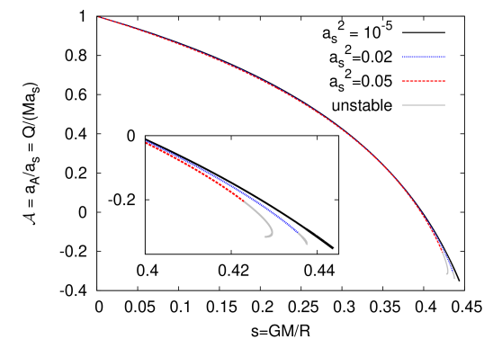
Refer to caption
Refer to caption
Figure 3: Top: A comparison of 𝒜=aA/as=Q/(Mas)𝒜subscript𝑎𝐴subscript𝑎𝑠𝑄𝑀subscript𝑎𝑠\mathcal{A}=a_{{\scriptscriptstyle A}}/a_{s}=Q/(Ma_{s}) vs s=GM/R𝑠𝐺𝑀𝑅s=GM/R for incompressible stars in Brans-Dicke theory, for various values of assubscript𝑎𝑠a_{s}. The curves start at s=0𝑠0s=0, 𝒜=1𝒜1\mathcal{A}=1 where p00subscript𝑝00p_{0}\to 0, and terminate where p0subscript𝑝0p_{0}\to\infty. Bottom: The same quantity comparing incompressible stars with two kinds of neutron-star equations of state (relativistic polytropes) given in [18], using Brans-Dicke theory to leading order in assubscript𝑎𝑠a_{s}.

The dependence of aA/a0subscript𝑎𝐴subscript𝑎0a_{\scriptscriptstyle A}/a_{0} on s𝑠s is shown in Figure 3 for several choices of a0=assubscript𝑎0subscript𝑎𝑠a_{0}=a_{s} in the special case of Brans-Dicke theory (bs=0subscript𝑏𝑠0b_{s}=0), using for illustration an incompressible star equation of state (see §5, below). Each curve can be parametrized by p0subscript𝑝0p_{0}. The starting point is at s=0𝑠0s=0, 𝒜=1𝒜1\mathcal{A}=1 when p00subscript𝑝00p_{0}\to 0, and the endpoint is reached in the limit p0p0maxsubscript𝑝0superscriptsubscript𝑝0maxp_{0}\to p_{0}^{\rm max}. These curves show that the small-a0subscript𝑎0a_{0} limit works well in this case even out to very relativistic stars. Notice that aAsubscript𝑎𝐴a_{\scriptscriptstyle A} is in general smaller than a0subscript𝑎0a_{0}, with the suppression increasing for more relativistic stars.

Fig. (3) also compares the amount of this suppression for several other choices for the equation of state, indicating that the suppression for relativistic polytropes (more about which later) is under-estimated for incompressible stars, although they all agree in the non-relativistic limit (for which s(0)1much-less-thansubscript𝑠01s_{(0)}\ll 1), in agreement with intuition.

For incompressible stars aAsubscript𝑎𝐴a_{\scriptscriptstyle A} eventually becomes negative. As seen in the insert in Fig. (3), this change in sign takes place before the onset of instability, so there exist stable incompressible stars with aA<0subscript𝑎𝐴0a_{\scriptscriptstyle A}<0. The scalar interaction between two stars A𝐴A and B𝐵B is attractive if aAaB>0subscript𝑎𝐴subscript𝑎𝐵0a_{\scriptscriptstyle A}a_{\scriptscriptstyle B}>0, and repulsive if aAaB<0subscript𝑎𝐴subscript𝑎𝐵0a_{\scriptscriptstyle A}a_{\scriptscriptstyle B}<0. If at least one of A𝐴A, B𝐵B is an incompressible star, then both cases are possible. However, negative values of aAsubscript𝑎𝐴a_{\scriptscriptstyle A} are not seen for the more realistic equations of state, although these do approach aA=0subscript𝑎𝐴0a_{\scriptscriptstyle A}=0 when extremely relativistic. This should be compared with the corresponding universal result, Q=0𝑄0Q=0, found above for a static, spherically symmetric black hole.

Spontaneous Scalarization

In the above section, the scalar-coupling constraint was expanded in powers of a0subscript𝑎0a_{0}, and it was found that at leading order, aAsubscript𝑎𝐴a_{{\scriptscriptstyle A}} is a single-valued function of asubscript𝑎a_{\infty}. In this section, we take the expansion to next order, and demonstrate that aAsubscript𝑎𝐴a_{{\scriptscriptstyle A}} becomes a multi-valued function asubscript𝑎a_{\infty}. As a consequence, a0subscript𝑎0a_{0} and aAsubscript𝑎𝐴a_{\scriptscriptstyle A} can both be nonzero even when asubscript𝑎a_{\infty} vanishes. The phenomenon where Q/M𝑄𝑀Q/M is nonzero even though a=0subscript𝑎0a_{\infty}=0 is called spontaneous scalarization. To simplify notation, write

a=d1a0+d2a03+𝒪(a05),subscript𝑎subscript𝑑1subscript𝑎0subscript𝑑2superscriptsubscript𝑎03𝒪superscriptsubscript𝑎05\displaystyle a_{\infty}=d_{1}a_{0}+d_{2}a_{0}^{3}+\mathcal{O}(a_{0}^{5})\,, (101)
aA=e1a0+e2a03+𝒪(a05).subscript𝑎𝐴subscript𝑒1subscript𝑎0subscript𝑒2superscriptsubscript𝑎03𝒪superscriptsubscript𝑎05\displaystyle a_{{\scriptscriptstyle A}}=e_{1}a_{0}+e_{2}a_{0}^{3}+\mathcal{O}(a_{0}^{5})\,. (102)

Dropping terms of order a05superscriptsubscript𝑎05a_{0}^{5} and inverting equation (101) yields

a0=ωC++ω¯C,subscript𝑎0𝜔subscript𝐶¯𝜔subscript𝐶a_{0}=\omega C_{+}+\bar{\omega}C_{-}\,, (103)

where

C±=a2d2±D3,D=(a2d2)2+(d13d2)3,formulae-sequencesubscript𝐶plus-or-minus3plus-or-minussubscript𝑎2subscript𝑑2𝐷𝐷superscriptsubscript𝑎2subscript𝑑22superscriptsubscript𝑑13subscript𝑑23C_{\pm}=\sqrt[3]{\frac{a_{\infty}}{2d_{2}}\pm\sqrt{D}}\,,\qquad D=\left(\frac{a_{\infty}}{2d_{2}}\right)^{2}+\left(\frac{d_{1}}{3d_{2}}\right)^{3}\,, (104)

and ω=1,eiπ/3,eiπ/3𝜔1superscript𝑒𝑖𝜋3superscript𝑒𝑖𝜋3\omega=1,-e^{-i\pi/3},-e^{i\pi/3}. Thus,

aA=(ωC++ω¯C)e1+(ωC++ω¯C)3e2+𝒪(a05).subscript𝑎𝐴𝜔subscript𝐶¯𝜔subscript𝐶subscript𝑒1superscript𝜔subscript𝐶¯𝜔subscript𝐶3subscript𝑒2𝒪superscriptsubscript𝑎05a_{{\scriptscriptstyle A}}=(\omega C_{+}+\bar{\omega}C_{-})e_{1}+(\omega C_{+}+\bar{\omega}C_{-})^{3}e_{2}+\mathcal{O}(a_{0}^{5})\,. (105)

If D>0𝐷0D>0, then the ω=1𝜔1\omega=1 solution is real, and the other two solutions are complex. Thus, specification of asubscript𝑎a_{\infty} determines a unique stellar configuration.

If D<0𝐷0D<0, then all solutions are real. Thus, specification of asubscript𝑎a_{\infty} determines three stellar configurations.

In the limit a0subscript𝑎0a_{\infty}\to 0, the ω=1𝜔1\omega=1 solution vanishes, and the other two solutions become

a0=±d1d2.subscript𝑎0plus-or-minussubscript𝑑1subscript𝑑2a_{0}=\pm\sqrt{-\frac{d_{1}}{d_{2}}}\,. (106)

Therefore, whenever the quantity inside the square root is positive, there exist stellar configurations with a=0subscript𝑎0a_{\infty}=0 and

aA=±{(d1d2)1/2e1+(d1d2)3/2e2}+𝒪(a05).subscript𝑎𝐴plus-or-minussuperscriptsubscript𝑑1subscript𝑑212subscript𝑒1superscriptsubscript𝑑1subscript𝑑232subscript𝑒2𝒪superscriptsubscript𝑎05a_{{\scriptscriptstyle A}}=\pm\left\{\left(-\frac{d_{1}}{d_{2}}\right)^{1/2}e_{1}+\left(-\frac{d_{1}}{d_{2}}\right)^{3/2}e_{2}\right\}+\mathcal{O}(a_{0}^{5})\,. (107)

This is precisely the phenomenon of spontaneous scalarization.

The coefficients disubscript𝑑𝑖d_{i} and eisubscript𝑒𝑖e_{i} are functions of bssubscript𝑏𝑠b_{s} and p0subscript𝑝0p_{0}, and they also depend on the equation of state. The solution obtained in section 5.2 for incompressible stars can be used to calculate

d1subscript𝑑1\displaystyle d_{1} =\displaystyle= HeunG(a~,q~;α~,β~,γ~,δ~;Z)1+p01+3p0log(1+p01+3p0)HeunG(a~,q~;α~,β~,γ~,δ~;Z),HeunG~𝑎~𝑞~𝛼~𝛽~𝛾~𝛿𝑍1subscript𝑝013subscript𝑝01subscript𝑝013subscript𝑝0superscriptHeunG~𝑎~𝑞~𝛼~𝛽~𝛾~𝛿𝑍\displaystyle{\rm HeunG}(\tilde{a},\tilde{q};\tilde{\alpha},\tilde{\beta},\tilde{\gamma},\tilde{\delta};Z)-\frac{1+p_{0}}{1+3p_{0}}\log\left(\frac{1+p_{0}}{1+3p_{0}}\right){\rm HeunG^{\prime}}(\tilde{a},\tilde{q};\tilde{\alpha},\tilde{\beta},\tilde{\gamma},\tilde{\delta};Z)\,, (108)
e1subscript𝑒1\displaystyle e_{1} =\displaystyle= 1+p0bs(1+3p0)HeunG(a~,q~;α~,β~,γ~,δ~;Z),1subscript𝑝0subscript𝑏𝑠13subscript𝑝0superscriptHeunG~𝑎~𝑞~𝛼~𝛽~𝛾~𝛿𝑍\displaystyle\frac{1+p_{0}}{b_{s}(1+3p_{0})}{\rm HeunG^{\prime}}(\tilde{a},\tilde{q};\tilde{\alpha},\tilde{\beta},\tilde{\gamma},\tilde{\delta};Z)\,, (109)

where the arguments inside the Heun functions are given in equations (159)-(160), and Z=p0/(3p0+1)𝑍subscript𝑝03subscript𝑝01Z=p_{0}/(3p_{0}+1). Note that in the limit p00subscript𝑝00p_{0}\to 0, we have d11subscript𝑑11d_{1}\to 1 and e11subscript𝑒11e_{1}\to 1. In principle, the next coefficients d2subscript𝑑2d_{2} and e2subscript𝑒2e_{2} can be calculated using the solution found in section 5.3. However, the resulting expressions are very complicated.

It follows from equation (106) that the onset of scalarization implies d1=0subscript𝑑10d_{1}=0. Thus, all the points (bs,p0)subscript𝑏𝑠subscript𝑝0(b_{s},p_{0}) at which scalarization starts can be found by doing a root search of equation (108).

In figure (4), equation (108) is plotted versus p0subscript𝑝0p_{0}, for various negative values of bssubscript𝑏𝑠b_{s}. In all cases, d1subscript𝑑1d_{1} is a convex function of p0subscript𝑝0p_{0}, with one global minimum. If bs(4.329,0)subscript𝑏𝑠4.3290b_{s}\in(-4.329,0), then d1subscript𝑑1d_{1} never crosses zero, and there is no scalarization. If bs(,4.329)subscript𝑏𝑠4.329b_{s}\in(-\infty,-4.329), then d1subscript𝑑1d_{1} has two crossings of zero, which correspond to the scalarization which has been extensively studied in the literature.

In figure (5), equation (108) is plotted versus p0subscript𝑝0p_{0}, for various positive values of bssubscript𝑏𝑠b_{s}. In all cases, d1subscript𝑑1d_{1} is an oscillatory function of p0subscript𝑝0p_{0}, and there are multiple regions of scalarization. We have verified numerically that scalarization does actually occur when d1<0subscript𝑑10d_{1}<0. However, application of of the stability criterion of §3.2 shows that these scalarized stars are unstable whenever bs>0subscript𝑏𝑠0b_{s}>0.

Refer to caption
Figure 4: The coefficient d1subscript𝑑1d_{1} plotted versus p0subscript𝑝0p_{0}, for constant-density stars, for several choices of bs<0subscript𝑏𝑠0b_{s}<0. Scalarization becomes possible for bs<4.329subscript𝑏𝑠4.329b_{s}<-4.329.
Refer to caption
Figure 5: The coefficient d1subscript𝑑1d_{1} plotted versus p0subscript𝑝0p_{0}, for constant-density stars, for several choices of bs>0subscript𝑏𝑠0b_{s}>0. There are multiple regions of scalarization.

4.3 Non-relativistic polytropes

As an example for which the scalar-field dependence of the above constraints can be more explicitly explored, consider the case of Newtonian polytropes discussed §3.4 with equation of state P=Kρ1+1/χ𝑃𝐾superscript𝜌11𝜒P=K\rho^{1+1/\chi}. In this case for weak central coupling the scalar field, φ𝜑\varphi, and the dimensionless density, θ=(ρ/ρ0)1/χ𝜃superscript𝜌subscript𝜌01𝜒\theta=(\rho/\rho_{0})^{1/\chi}, can be expanded in a02superscriptsubscript𝑎02a_{0}^{2}, bssubscript𝑏𝑠b_{s}, as well as the parameter ζ=(1+χ)Kρ01/χ=(1+χ)P0/ρ0=(1+χ)p0𝜁1𝜒𝐾superscriptsubscript𝜌01𝜒1𝜒subscript𝑃0subscript𝜌01𝜒subscript𝑝0\zeta=(1+\chi)K\rho_{0}^{1/\chi}=(1+\chi)P_{0}/\rho_{0}=(1+\chi)p_{0}:

θ𝜃\displaystyle\theta =\displaystyle= iθ(i)a02i=i,jθ(i,j)a02ibsj=i,j,kθ(i,j,k)a02ibsjζk,subscript𝑖subscript𝜃𝑖superscriptsubscript𝑎02𝑖subscript𝑖𝑗subscript𝜃𝑖𝑗superscriptsubscript𝑎02𝑖superscriptsubscript𝑏𝑠𝑗subscript𝑖𝑗𝑘subscript𝜃𝑖𝑗𝑘superscriptsubscript𝑎02𝑖superscriptsubscript𝑏𝑠𝑗superscript𝜁𝑘\displaystyle\sum_{i}\theta_{(i)}a_{0}^{2i}=\sum_{i,j}\theta_{(i,j)}\,a_{0}^{2i}\,b_{s}^{j}=\sum_{i,j,k}\theta_{(i,j,k)}\,a_{0}^{2i}\,b_{s}^{j}\,\zeta^{k}\ , (110)
φ𝜑\displaystyle\varphi =\displaystyle= iφ(i)a02i=i,jφ(i,j)a02ibsj=i,j,kφ(i,j,k)a02ibsjζk.subscript𝑖subscript𝜑𝑖superscriptsubscript𝑎02𝑖subscript𝑖𝑗subscript𝜑𝑖𝑗superscriptsubscript𝑎02𝑖superscriptsubscript𝑏𝑠𝑗subscript𝑖𝑗𝑘subscript𝜑𝑖𝑗𝑘superscriptsubscript𝑎02𝑖superscriptsubscript𝑏𝑠𝑗superscript𝜁𝑘\displaystyle\sum_{i}\varphi_{(i)}a_{0}^{2i}=\sum_{i,j}\varphi_{(i,j)}\,a_{0}^{2i}\,b_{s}^{j}=\sum_{i,j,k}\varphi_{(i,j,k)}\,a_{0}^{2i}\,b_{s}^{j}\,\zeta^{k}\ . (111)

We show below that ζ1much-less-than𝜁1\zeta\ll 1 for the polytropes of practical interest, such as white dwarfs and main-sequence stars.

In the limit a02=0superscriptsubscript𝑎020a_{0}^{2}=0, eqs. (81) – (82) become

θ′′superscript𝜃′′\displaystyle{\theta}^{\prime\prime} =\displaystyle= 2θwθχ,2superscript𝜃𝑤superscript𝜃𝜒\displaystyle-\frac{2{\theta}^{\prime}}{w}-\theta^{\chi}\ , (112)
φ′′superscript𝜑′′\displaystyle{\varphi}^{\prime\prime} =\displaystyle= 2φw+ζθχ[1+wφ+bsφ].2superscript𝜑𝑤𝜁superscript𝜃𝜒delimited-[]1𝑤superscript𝜑subscript𝑏𝑠𝜑\displaystyle-\frac{2{\varphi}^{\prime}}{w}+\zeta\theta^{\chi}[1+w{\varphi}^{\prime}+b_{s}\varphi]\ . (113)

where for later notational convenience we use primes in this section to denote differentiation with respect to w𝑤w. Equation (112) is called the Lane-Emden equation, and its solutions are well-studied because of its important role in the theory of stellar structure. It can be solved analytically when χ=0,1,5𝜒015\chi=0,1,5 [64]. The solutions of the Lane-Emden equation with initial conditions (76) are called Lane-Emden functions, and are denoted by Θχ(w)subscriptΘ𝜒𝑤\Theta_{\chi}(w). Thus,

θ(0)(w)=Θχ(w).subscript𝜃0𝑤subscriptΘ𝜒𝑤\theta_{(0)}(w)=\Theta_{\chi}(w)\ . (114)

If we now take bs=0subscript𝑏𝑠0b_{s}=0 then equation (113) can be solved for φ𝜑\varphi in terms of θ𝜃\theta, giving

φ(0,0)subscriptsuperscript𝜑00\displaystyle{\varphi^{\prime}_{(0,0)}} =\displaystyle= ζw2eζ(wΘχ)w(w^2Θχ)eζ(w^Θχ)dw^𝜁superscript𝑤2superscript𝑒𝜁superscript𝑤subscriptΘ𝜒superscript𝑤superscriptsuperscript^𝑤2superscriptsubscriptΘ𝜒superscript𝑒𝜁superscript^𝑤subscriptΘ𝜒d^𝑤\displaystyle-\frac{\zeta}{w^{2}}e^{-\zeta(w\Theta_{\chi})^{\prime}}\int^{w}(\hat{w}^{2}{\Theta}_{\chi}^{\prime})^{\prime}e^{\zeta(\hat{w}\Theta_{\chi})^{\prime}}{\hbox{d}}\hat{w}\ (115)
=\displaystyle= 1w+1w2eζ(wΘχ)weζ(w^Θχ)dw^.1𝑤1superscript𝑤2superscript𝑒𝜁superscript𝑤subscriptΘ𝜒superscript𝑤superscript𝑒𝜁superscript^𝑤subscriptΘ𝜒d^𝑤\displaystyle-\frac{1}{w}+\frac{1}{w^{2}}e^{-\zeta(w\Theta_{\chi})^{\prime}}\int^{w}e^{\zeta(\hat{w}\Theta_{\chi})^{\prime}}{\hbox{d}}\hat{w}\,. (116)

Expanding this in powers of ζ𝜁\zeta then yields

φ(0,0)ζ(1Θχ)+𝒪(ζ2).similar-to-or-equalssubscript𝜑00𝜁1subscriptΘ𝜒𝒪superscript𝜁2\varphi_{(0,0)}\simeq\zeta(1-\Theta_{\chi})+\mathcal{O}(\zeta^{2})\,. (117)

and so

φ(0,0,0)=0andφ(0,0,1)=1Θχ.formulae-sequencesubscript𝜑0000andsubscript𝜑0011subscriptΘ𝜒\varphi_{(0,0,0)}=0\quad\hbox{and}\quad\varphi_{(0,0,1)}=1-\Theta_{\chi}\ . (118)

Expanding the matching equations, eqs. (87) – (89) in powers of a02superscriptsubscript𝑎02a_{0}^{2}, bssubscript𝑏𝑠b_{s} and ζ𝜁\zeta similarly yields

GMR𝐺𝑀𝑅\displaystyle\frac{GM}{R} similar-to-or-equals\displaystyle\simeq ζWΘχ(W)+𝒪(a02),𝜁𝑊subscriptsuperscriptΘ𝜒𝑊𝒪superscriptsubscript𝑎02\displaystyle-\zeta W{\Theta^{\prime}}_{\chi}(W)+\mathcal{O}(a_{0}^{2})\,, (119)
QMa0𝑄𝑀subscript𝑎0\displaystyle\frac{Q}{Ma_{0}} similar-to-or-equals\displaystyle\simeq 1+𝒪(a02)+𝒪(bs)+𝒪(ζ),1𝒪superscriptsubscript𝑎02𝒪subscript𝑏𝑠𝒪𝜁\displaystyle 1+\mathcal{O}(a_{0}^{2})+\mathcal{O}(b_{s})+\mathcal{O}(\zeta)\,, (120)
ϕϕ0a0subscriptitalic-ϕsubscriptitalic-ϕ0subscript𝑎0\displaystyle\frac{\phi_{\infty}-\phi_{0}}{a_{0}} similar-to-or-equals\displaystyle\simeq ζ[1Θχ(W)WΘχ(W)]+𝒪(a02)+𝒪(bs)+𝒪(ζ2).𝜁delimited-[]1subscriptΘ𝜒𝑊𝑊subscriptsuperscriptΘ𝜒𝑊𝒪superscriptsubscript𝑎02𝒪subscript𝑏𝑠𝒪superscript𝜁2\displaystyle\zeta\Bigl{[}1-\Theta_{\chi}(W)-W{\Theta^{\prime}}_{\chi}(W)\Bigr{]}+\mathcal{O}(a_{0}^{2})+\mathcal{O}(b_{s})+\mathcal{O}(\zeta^{2})\,. (121)

Notice in particular that eq. (120) implies that

aAa0[1+𝒪(a02)+𝒪(bs)+𝒪(ζ)],similar-to-or-equalssubscript𝑎𝐴subscript𝑎0delimited-[]1𝒪subscriptsuperscript𝑎20𝒪subscript𝑏𝑠𝒪𝜁a_{A}\simeq a_{0}\Bigl{[}1+\mathcal{O}(a^{2}_{0})+\mathcal{O}(b_{s})+\mathcal{O}(\zeta)\Bigr{]}\,, (122)

which is consistent with the limit aAa(ϕ)subscript𝑎𝐴𝑎subscriptitalic-ϕa_{A}\to a(\phi_{\infty}) for weakly self-gravitating stars. Similarly, equation (119) can be re-written as

GM𝐺𝑀\displaystyle GM =\displaystyle= ζrsW2Θχ+𝒪(a02)𝜁subscript𝑟𝑠superscript𝑊2subscriptsuperscriptΘ𝜒𝒪superscriptsubscript𝑎02\displaystyle-\zeta r_{s}W^{2}\Theta^{\prime}_{\chi}+\mathcal{O}(a_{0}^{2}) (123)
=\displaystyle= W2Θχ(W)[ρ0(3χ)/2χA02K3(χ+1)34πG]+𝒪(a02).superscript𝑊2subscriptsuperscriptΘ𝜒𝑊delimited-[]superscriptsubscript𝜌03𝜒2𝜒subscriptsuperscript𝐴20superscript𝐾3superscript𝜒134𝜋𝐺𝒪superscriptsubscript𝑎02\displaystyle-W^{2}{\Theta}^{\prime}_{\chi}(W)\;\left[\frac{\rho_{0}^{(3-\chi)/2\chi}}{A^{2}_{0}}\sqrt{\frac{K^{3}(\chi+1)^{3}}{4\pi G}}\right]+\mathcal{O}(a_{0}^{2})\,.

which is independent of ρ0subscript𝜌0\rho_{0}, as advertised, when χ=3𝜒3\chi=3.

To get an idea about the validity of the ζ𝜁\zeta expansion, we close this section by estimating its size for the examples of white dwarfs and main-sequence polytropes.

White dwarfs

A white dwarf can be modeled by a degenerate fermion gas which satisfies in the ultra-relativistic limit the polytropic equation of state, eq. (70), with

K=31/3π2/34(Yemb)4/3andχ=3.formulae-sequence𝐾superscript313superscript𝜋234superscriptsubscript𝑌𝑒subscript𝑚𝑏43and𝜒3K=\frac{3^{1/3}\pi^{2/3}}{4}\left(\frac{Y_{e}}{m_{b}}\right)^{4/3}\quad\hbox{and}\quad\chi=3\,. (124)

Here Yesubscript𝑌𝑒Y_{e} is the number of electrons per nucleon and mbsubscript𝑚𝑏m_{b} is the average nucleon mass [61]. Although the fermion gas is highly relativistic, the gravitational field generated by it is not strong, allowing use of the non-relativistic expressions developed above.

The typical central densities of white dwarfs are ρ0(1071014)kgm3similar-tosubscript𝜌0superscript107superscript1014kgsuperscriptm3\rho_{0}\sim(10^{7}\ldots 10^{14})\;{\rm kg}\,{\rm m}^{-3} [61], corresponding to 105<ζ<102<superscript105𝜁<superscript10210^{-5}\mathrel{\raise 1.29167pt\hbox{$<$\kern-8.50006pt\lower 4.30554pt\hbox{$\sim$}}}\zeta\mathrel{\raise 1.29167pt\hbox{$<$\kern-8.50006pt\lower 4.30554pt\hbox{$\sim$}}}10^{-2} for Ye=12subscript𝑌𝑒12Y_{e}=\frac{1}{2}. This shows that a perturbative expansion in ζ𝜁\zeta is likely a good approximation for white dwarfs.

Since the ultra-relativistic limit of the fermion gas is used, the mass calculated below using the matching conditions — i.e. equation (123) — is greater than the actual mass of the white dwarf. It is instead to be regarded as the Chandrasekhar limit: an upper bound on the mass of white dwarfs. Because χ=3𝜒3\chi=3 its value turns out to be independent of ρ0subscript𝜌0\rho_{0}, and for Ye=12subscript𝑌𝑒12Y_{e}=\frac{1}{2}, its value is approximately 1.4M1.4subscript𝑀direct-product1.4M_{\odot} [62].

Main-sequence models

In the Eddington stellar model, a star is regarded as an ideal gas whose energy is transported by radiation, and it is assumed that the gas makes up a fixed fraction of the total pressure, β:=Pgas/P=constassign𝛽subscript𝑃gas𝑃const\beta:={P_{\rm gas}}/{P}={\rm const}. Here Pgassubscript𝑃gasP_{\rm gas} is the pressure of the ideal gas, and the total pressure is P=Pgas+Prad𝑃subscript𝑃gassubscript𝑃radP=P_{\rm gas}+P_{\rm rad}, where Pradsubscript𝑃radP_{\rm rad} is the radiation pressure. The Eddington model leads to a polytropic equation of state with

K=[45π2kB4(Rgμ)41ββ4]1/3andχ=3,formulae-sequence𝐾superscriptdelimited-[]45superscript𝜋2superscriptsubscript𝑘𝐵4superscriptsubscript𝑅𝑔𝜇41𝛽superscript𝛽413and𝜒3K=\left[\frac{45}{\pi^{2}k_{\scriptscriptstyle B}^{4}}\left(\frac{R_{g}}{\mu}\right)^{4}\frac{1-\beta}{\beta^{4}}\right]^{1/3}\quad\hbox{and}\quad\chi=3\,, (125)

where Rgsubscript𝑅𝑔R_{g} is the universal gas constant, μ𝜇\mu is the molar mass of the ideal gas and kBsubscript𝑘𝐵k_{\scriptscriptstyle B} is Boltzmann’s constant [63]. Main-sequence stars can be approximately described by the Eddington standard model, even though convection also plays a role in heat transfer for more realistic models.

For a more accurate single-polytrope model of the Sun, χ=3.35𝜒3.35\chi=3.35 and ζ105similar-to𝜁superscript105\zeta\sim 10^{-5} [69], so the perturbative expansion in ζ𝜁\zeta remains a good approximation.

5 Incompressible stars

We now specialize the discussions of the previous sections to the special case of an incompressible star, for which the stellar density, ρ𝜌\rho, is constant. Since constant density can only be consistent with the pressure gradients required for hydrostatic equilibrium if pp(ρ)𝑝𝑝𝜌p\neq p(\rho), we no longer impose this kind of equation of state. (It is not necessary in any case, since the closure of the field equations is now accomplished by the incompressibility condition, ρ(r)ρ0𝜌𝑟subscript𝜌0\rho(r)\equiv\rho_{0}.)

The purpose of this exercise is to have a toy example for which all of the above manipulations can be simply carried through explicitly in closed form. Performing the same exercise for GR provides an interesting example that displays the main features of relativistic structure, including the existence of a maximum compactness for a star, s(0)49subscript𝑠049s_{(0)}\leq\frac{4}{9}, that can be supported against gravitational collapse. The maximum that is found for incompressible stars turns out to provide an upper bound to the maximum compactness that can be achieved with other equations of state.

Several earlier works have numerically investigated incompressible stars in scalar-tensor gravity [36, 40, 45], but our quasi-analytical treatment of these stars is new.

5.1 Incompressible stars with quasi-Brans/Dicke scalars

We cut right to the chase and specialize directly to qBD scalars, for which a(ϕ)=as+bsϕ𝑎italic-ϕsubscript𝑎𝑠subscript𝑏𝑠italic-ϕa(\phi)=a_{s}+b_{s}\phi, since this case is broad enough to be of wide interest, but restricted enough to be explored in detail.

Field equations

Taking the equation of state to be ρ=ρ0𝜌subscript𝜌0\rho=\rho_{0}, or ϱ(p)=1italic-ϱ𝑝1\varrho(p)=1, equations (47) – (49) become

μ˙˙𝜇\displaystyle\dot{\mu} =\displaystyle= μ2u+14e4a02φ(1+bsφ/2)+a02u(12μ)φ˙2𝜇2𝑢14superscript𝑒4superscriptsubscript𝑎02𝜑1subscript𝑏𝑠𝜑2superscriptsubscript𝑎02𝑢12𝜇superscript˙𝜑2\displaystyle-\frac{\mu}{2u}+\frac{1}{4}\,e^{4a_{0}^{2}\varphi(1+b_{s}\varphi/2)}+a_{0}^{2}\,u(1-2\mu)\dot{\varphi}^{2} (126)
p˙˙𝑝\displaystyle\dot{p} =\displaystyle= (1+p)[μ2u(12μ)+p4(12μ)e4a02φ(1+bsφ/2)+a02φ˙(1+uφ˙+bsφ)]1𝑝delimited-[]𝜇2𝑢12𝜇𝑝412𝜇superscript𝑒4superscriptsubscript𝑎02𝜑1subscript𝑏𝑠𝜑2superscriptsubscript𝑎02˙𝜑1𝑢˙𝜑subscript𝑏𝑠𝜑\displaystyle-(1+p)\left[\frac{\mu}{2u(1-2\mu)}+\frac{p}{4(1-2\mu)}\,e^{4a_{0}^{2}\varphi(1+b_{s}\varphi/2)}+a_{0}^{2}\,\dot{\varphi}(1+u\dot{\varphi}+b_{s}\varphi)\right] (127)
φ¨¨𝜑\displaystyle\ddot{\varphi} =\displaystyle= (34μ)φ˙2u(12μ)+e4a02φ(1+bsφ/2)8u(12μ)[(1+bsφ)(13p)+2(1p)uφ˙].34𝜇˙𝜑2𝑢12𝜇superscript𝑒4superscriptsubscript𝑎02𝜑1subscript𝑏𝑠𝜑28𝑢12𝜇delimited-[]1subscript𝑏𝑠𝜑13𝑝21𝑝𝑢˙𝜑\displaystyle-\frac{(3-4\mu)\dot{\varphi}}{2u(1-2\mu)}+\frac{e^{4a_{0}^{2}\varphi(1+b_{s}\varphi/2)}}{8u(1-2\mu)}\Bigl{[}(1+b_{s}\varphi)(1-3p)+2(1-p)u\dot{\varphi}\Bigr{]}\,. (128)

Similarly, the function f(p)𝑓𝑝f(p) defined in eq. (23) becomes

f(p)=ln(1+p1+p0),𝑓𝑝1𝑝1subscript𝑝0f(p)=\ln\left(\frac{1+p}{1+p_{0}}\right)\,, (129)

and so the baryon number density, n(r)𝑛𝑟n(r), computed from eq. (41) is also constant, n=n0𝑛subscript𝑛0n=n_{0}. The function \mathcal{M} defined in eq. (51) similarly becomes

\displaystyle\mathcal{M} =\displaystyle= 0Uduu12μexp[3a02φ(1+bsφ2)].superscriptsubscript0𝑈d𝑢𝑢12𝜇3superscriptsubscript𝑎02𝜑1subscript𝑏𝑠𝜑2\displaystyle\int_{0}^{U}{\hbox{d}}u\sqrt{\frac{u}{1-2\mu}}\exp\left[3a_{0}^{2}\varphi\left(1+\frac{b_{s}\varphi}{2}\right)\right]\,. (130)

5.2 Perturbative solutions: leading order

Because the GR problem can be explicitly integrated for incompressible stars, equations (126) – (128) can be solved analytically when a02=0superscriptsubscript𝑎020a_{0}^{2}=0. The zeroth-order profiles, μ(0)subscript𝜇0\mu_{(0)} and p(0)subscript𝑝0p_{(0)}, are given by [65, 66]

μ(0)(u)subscript𝜇0𝑢\displaystyle\mu_{(0)}(u) =\displaystyle= u6,𝑢6\displaystyle\frac{u}{6}\,, (131)
p(0)(u)subscript𝑝0𝑢\displaystyle p_{(0)}(u) =\displaystyle= (1+3p0)1u/3(1+p0)3(1+p0)(1+3p0)1u/3,13subscript𝑝01𝑢31subscript𝑝031subscript𝑝013subscript𝑝01𝑢3\displaystyle\frac{(1+3p_{0})\sqrt{1-u/3}-(1+p_{0})}{3(1+p_{0})-(1+3p_{0})\sqrt{1-u/3}}\,, (132)

as a function of the central pressure p0subscript𝑝0p_{0}. We return to computing the profile, φ(u)𝜑𝑢\varphi(u), below.

At leading order the stellar radius is determined as the zero of p(0)subscript𝑝0p_{(0)}, which vanishes at u=U(0)𝑢subscript𝑈0u=U_{(0)} where

U(0)=12p0(1+2p0)(1+3p0)2,subscript𝑈012subscript𝑝012subscript𝑝0superscript13subscript𝑝02U_{(0)}=\frac{12p_{0}(1+2p_{0})}{(1+3p_{0})^{2}}\,, (133)

corresponding to the radius r=R(0)𝑟subscript𝑅0r=R_{(0)} with

R(0)=2A02(1+3p0)3p0(1+2p0)8πGρ0.subscript𝑅02subscriptsuperscript𝐴2013subscript𝑝03subscript𝑝012subscript𝑝08𝜋𝐺subscript𝜌0R_{(0)}=\frac{2}{A^{2}_{0}(1+3p_{0})}\sqrt{\frac{3p_{0}(1+2p_{0})}{8\pi G\rho_{0}}}\,. (134)

The leading components of the functions relevant to matching to the exterior solutions — i.e. \mathcal{F}, 𝒜𝒜\mathcal{A}, s𝑠s and \mathcal{M} — are

(0)subscript0\displaystyle\mathcal{F}_{(0)} =\displaystyle= φ(0)12(1+p01+3p0)2ln(1+p01+3p0)φ˙(0),subscript𝜑absent012superscript1subscript𝑝013subscript𝑝021subscript𝑝013subscript𝑝0subscript˙𝜑absent0\displaystyle\varphi_{\star(0)}-12\left(\frac{1+p_{0}}{1+3p_{0}}\right)^{2}\ln\left(\frac{1+p_{0}}{1+3p_{0}}\right)\dot{\varphi}_{\star(0)}\,, (135)
𝒜(0)subscript𝒜0\displaystyle\mathcal{A}_{(0)} =\displaystyle= 12(1+p01+3p0)2φ˙(0),12superscript1subscript𝑝013subscript𝑝02subscript˙𝜑absent0\displaystyle 12\left(\frac{1+p_{0}}{1+3p_{0}}\right)^{2}\dot{\varphi}_{\star(0)}\,, (136)
s(0)subscript𝑠0\displaystyle s_{(0)} =\displaystyle= 2p0(1+2p0)(1+3p0)2,2subscript𝑝012subscript𝑝0superscript13subscript𝑝02\displaystyle\frac{2p_{0}(1+2p_{0})}{(1+3p_{0})^{2}}\,, (137)
(0)subscript0\displaystyle\mathcal{M}_{(0)} =\displaystyle= 33{arccos(1+p01+3p0)2(1+p0)p0(1+2p0)(1+3p0)2},331subscript𝑝013subscript𝑝021subscript𝑝0subscript𝑝012subscript𝑝0superscript13subscript𝑝02\displaystyle 3\sqrt{3}\left\{\arccos\left(\frac{1+p_{0}}{1+3p_{0}}\right)-2\frac{(1+p_{0})\sqrt{p_{0}(1+2p_{0})}}{(1+3p_{0})^{2}}\right\}\,, (138)

where, as before, the subscript ‘\star’ denotes evaluation at u=U𝑢𝑈u=U, so φ(0):=φ(0)(U(0))assignsubscript𝜑absent0subscript𝜑0subscript𝑈0\varphi_{\star(0)}:=\varphi_{(0)}(U_{(0)}).

Equation (137) implies that the compactness is an increasing function of p0subscript𝑝0p_{0}, which vanishes when p0=0subscript𝑝00p_{0}=0 and asymptotes to 4949\frac{4}{9} as p0subscript𝑝0p_{0}\to\infty. Thus we reproduce the GR result 0s(0)490subscript𝑠0490\leq s_{(0)}\leq\frac{4}{9} for constant-density stars. This prediction gets modified once O(a02)𝑂superscriptsubscript𝑎02O(a_{0}^{2}) corrections are included, however, as is discussed in detail in the next section.

The mass-radius constraint, eq. (97), in this case becomes

s=GMR=4πGρ03A4R2+𝒪(a02),𝑠𝐺𝑀𝑅4𝜋𝐺subscript𝜌03subscriptsuperscript𝐴4superscript𝑅2𝒪subscriptsuperscript𝑎20s=\frac{GM}{R}=\frac{4\pi G\rho_{0}}{3}A^{4}_{\infty}R^{2}+\mathcal{O}(a^{2}_{0})\,, (139)

which states MR3proportional-to𝑀superscript𝑅3M\propto R^{3}, as might be expected for constant density. This behaviour is seen explicitly in the as=0subscript𝑎𝑠0a_{s}=0 curve in Fig. (2).

The scalar-coupling constraint, eq. (100), similarly becomes

aAsubscript𝑎𝐴\displaystyle a_{{\scriptscriptstyle A}} =\displaystyle= 12a(12s)φ˙(0)1+bsφ(0)6bs(12s)ln(12s)φ˙(0)+𝒪(a03),12subscript𝑎12𝑠subscript˙𝜑absent01subscript𝑏𝑠subscript𝜑absent06subscript𝑏𝑠12𝑠12𝑠subscript˙𝜑absent0𝒪subscriptsuperscript𝑎30\displaystyle\frac{12a_{\infty}(1-2s)\dot{\varphi}_{\star(0)}}{1+b_{s}\varphi_{\star(0)}-6b_{s}(1-2s)\ln(1-2s)\dot{\varphi}_{\star(0)}}+\mathcal{O}(a^{3}_{0})\,, (140)

where

p0=13s12s9s4+𝒪(a02)subscript𝑝013𝑠12𝑠9𝑠4𝒪subscriptsuperscript𝑎20p_{0}=\frac{1-3s-\sqrt{1-2s}}{9s-4}+\mathcal{O}(a^{2}_{0}) (141)

should be substituted into φ(0)subscript𝜑absent0\varphi_{\star{(0)}} and φ˙(0)subscript˙𝜑absent0\dot{\varphi}_{\star{(0)}} on the right-hand side. Since further progress requires knowing the scalar profile, we next turn to solving its field equation.

Scalar profile in Brans-Dicke theory (when bs=0subscript𝑏𝑠0b_{s}=0)

If bs=0subscript𝑏𝑠0b_{s}=0, then the model reduces to Brans-Dicke theory, and a(ϕ)a0=as𝑎italic-ϕsubscript𝑎0subscript𝑎𝑠a(\phi)\equiv a_{0}=a_{s}. Equation (128) with a02=0superscriptsubscript𝑎020a_{0}^{2}=0 becomes a first-order linear differential equation for φ˙˙𝜑\dot{\varphi}, which can be solved analytically:

φ˙(0)(u)=27(1+p0)(arcsinu/3u/31u/3)4(1+3p0)u12u1u/3(3(1+p0)(1+3p0)1u/3).subscript˙𝜑0𝑢271subscript𝑝0𝑢3𝑢31𝑢3413subscript𝑝0𝑢12𝑢1𝑢331subscript𝑝013subscript𝑝01𝑢3\dot{\varphi}_{(0)}(u)=\frac{27(1+p_{0})\left(\frac{\arcsin\sqrt{u/3}}{\sqrt{u/3}}-\sqrt{1-u/3}\right)-4(1+3p_{0})u}{12u\sqrt{1-u/3}(3(1+p_{0})-(1+3p_{0})\sqrt{1-u/3})}\,. (142)

Integrating this expression once more with respect to u𝑢u then gives

φ(0)subscript𝜑0\displaystyle\varphi_{(0)} =\displaystyle= 18(2+3p0)[(9p0+5)(3p01)ln(3(1+p0)(1+3p0)1u/3)\displaystyle\frac{1}{8(2+3p_{0})}\biggl{[}(9p_{0}+5)(3p_{0}-1)\ln\left(3(1+p_{0})-(1+3p_{0})\sqrt{1-u/3}\right) (143)
9(1+p0)(1+3p0+3(1+p0)1u/3)arcsinu/3u/3]\displaystyle\hphantom{\frac{1}{8(2+3p_{0})}\biggl{[}}-9(1+p_{0})\left(1+3p_{0}+3(1+p_{0})\sqrt{1-u/3}\right)\frac{\arcsin{\sqrt{u/3}}}{\sqrt{u/3}}\biggr{]}
+9(1+3p0)2(1+p0)16(2+3p0)3/2[Li2(λ)Li2(λ+)+iln(1λ1λ+)arcsinu/3],9superscript13subscript𝑝021subscript𝑝016superscript23subscript𝑝032delimited-[]subscriptLi2subscript𝜆subscriptLi2subscript𝜆𝑖1subscript𝜆1subscript𝜆𝑢3\displaystyle+\frac{9(1+3p_{0})^{2}(1+p_{0})}{16(2+3p_{0})^{3/2}}\biggl{[}{\rm Li}_{2}(\lambda_{-})-{\rm Li}_{2}(\lambda_{+})+i\ln\left(\frac{1-\lambda_{-}}{1-\lambda_{+}}\right)\arcsin{\sqrt{u/3}}\biggr{]}\,,

where

λ±:=(1+3p0)(1u/3+iu/3)3(1+p0)±22+3p0|λ±|eiarcsinu/3,assignsubscript𝜆plus-or-minus13subscript𝑝01𝑢3𝑖𝑢3plus-or-minus31subscript𝑝0223subscript𝑝0subscript𝜆plus-or-minussuperscript𝑒𝑖𝑢3\lambda_{\pm}:=\frac{(1+3p_{0})(\sqrt{1-u/3}+i\sqrt{u/3})}{3(1+p_{0})\pm 2\sqrt{2+3p_{0}}}\equiv|\lambda_{\pm}|e^{i\arcsin\sqrt{u/3}}\,, (144)

and

Li2(z)=k=1zkk2subscriptLi2𝑧superscriptsubscript𝑘1superscript𝑧𝑘superscript𝑘2{\rm Li}_{2}(z)=\sum_{k=1}^{\infty}\frac{z^{k}}{k^{2}} (145)

is the dilogarithm function.

By using the identity [67]

k=1pksin(kx)=psinx12pcosx+p2,superscriptsubscript𝑘1superscript𝑝𝑘𝑘𝑥𝑝𝑥12𝑝𝑥superscript𝑝2\sum_{k=1}^{\infty}p^{k}\sin(kx)=\frac{p\sin x}{1-2p\cos x+p^{2}}\,, (146)

it can be shown that the imaginary part of (143) is constant, and can thus be absorbed into an integration constant. The final normalized and manifestly-real expression for φ(0)subscript𝜑0\varphi_{(0)} is then

φ(0)(u)subscript𝜑0𝑢\displaystyle\varphi_{(0)}(u) =\displaystyle= 18(2+3p0)[(9p0+5)(3p01)log(32(1+p0)12(1+3p0)1u/3)\displaystyle\frac{1}{8(2+3p_{0})}\biggl{[}(9p_{0}+5)(3p_{0}-1)\log\left(\frac{3}{2}(1+p_{0})-\frac{1}{2}(1+3p_{0})\sqrt{1-u/3}\right) (147)
9(1+p0)(1+3p0+3(1+p0)1u/3)arcsinu/3u/3]\displaystyle\hphantom{\frac{1}{8(2+3p_{0})}\biggl{[}}-9(1+p_{0})\left(1+3p_{0}+3(1+p_{0})\sqrt{1-u/3}\right)\frac{\arcsin{\sqrt{u/3}}}{\sqrt{u/3}}\biggr{]}
+9(1+3p0)2(1+p0)16(2+3p0)3/2[arctan(2(2+3p0)u/31+3p03(1+p0)1u/3)arcsinu/3\displaystyle+\frac{9(1+3p_{0})^{2}(1+p_{0})}{16(2+3p_{0})^{3/2}}\biggl{[}\arctan\left(\frac{2\sqrt{(2+3p_{0})u/3}}{1+3p_{0}-3(1+p_{0})\sqrt{1-u/3}}\right)\arcsin\sqrt{u/3}
+[Li2(λ)Li2(|λ|)Li2(λ+)+Li2(|λ+|)]]\displaystyle\hphantom{+\frac{9(1+3p_{0})^{2}(1+p_{0})}{16(2+3p_{0})^{3/2}}\biggl{[}}+\Re\left[{\rm Li}_{2}(\lambda_{-})-{\rm Li}_{2}(|\lambda_{-}|)-{\rm Li}_{2}(\lambda_{+})+{\rm Li}_{2}(|\lambda_{+}|)\right]\biggr{]}
+94(1+p0).941subscript𝑝0\displaystyle+\frac{9}{4}(1+p_{0})\,.

If p0>13subscript𝑝013p_{0}>\frac{1}{\sqrt{3}}, then the inverse tangent in the above expression changes branch at the critical value

ucrit=4(2+3p0)3(1+p0)2<U(0),subscript𝑢crit423subscript𝑝03superscript1subscript𝑝02subscript𝑈0u_{\rm crit}=\frac{4(2+3p_{0})}{3(1+p_{0})^{2}}<U_{(0)}\,, (148)

so that φ(0)subscript𝜑0\varphi_{(0)} is a continuous function of u𝑢u.

Substituting equation (142) into (136) yields

𝒜(0)=9(1+p0)(1+3p0)216[p0(1+2p0)]3/2arccos(1+p01+3p0)41p02+34p0+98p0(1+2p0),subscript𝒜091subscript𝑝0superscript13subscript𝑝0216superscriptdelimited-[]subscript𝑝012subscript𝑝0321subscript𝑝013subscript𝑝041superscriptsubscript𝑝0234subscript𝑝098subscript𝑝012subscript𝑝0\mathcal{A}_{(0)}=\frac{9(1+p_{0})(1+3p_{0})^{2}}{16[p_{0}(1+2p_{0})]^{3/2}}\arccos\left(\frac{1+p_{0}}{1+3p_{0}}\right)-\frac{41p_{0}^{2}+34p_{0}+9}{8p_{0}(1+2p_{0})}\,, (149)

so the scalar-coupling constraint, eq. (140), can be explicitly evaluated,

aAsubscript𝑎𝐴\displaystyle a_{{\scriptscriptstyle A}} =\displaystyle= a0(5294s912s[27s14912s(23s)]8[s(59s+312s)]3/2arccos12s)subscript𝑎05294𝑠912𝑠delimited-[]27𝑠14912𝑠23𝑠8superscriptdelimited-[]𝑠59𝑠312𝑠3212𝑠\displaystyle a_{0}\left(\frac{5}{2}-\frac{9}{4s}-\frac{9\sqrt{1-2s}[27s-14-9\sqrt{1-2s}(2-3s)]}{8[s(5-9s+3\sqrt{1-2s})]^{3/2}}\arccos\sqrt{1-2s}\right) (150)
+𝒪(a03)𝒪superscriptsubscript𝑎03\displaystyle+\mathcal{O}(a_{0}^{3})
=\displaystyle= a0(165s+𝒪(s2))+𝒪(a03).subscript𝑎0165𝑠𝒪superscript𝑠2𝒪superscriptsubscript𝑎03\displaystyle a_{0}\left(1-\frac{6}{5}s+\mathcal{O}(s^{2})\right)+\mathcal{O}(a_{0}^{3})\,. (151)

This confirms that although aAa0subscript𝑎𝐴subscript𝑎0a_{\scriptscriptstyle A}\to a_{0} in the non-relativistic limit s0𝑠0s\to 0 — consistent with eq. (45) — it is in general depressed relative to a0subscript𝑎0a_{0} for relativistic systems, even when additional powers of a02superscriptsubscript𝑎02a_{0}^{2} are neglected.

Notice that in the opposite limit we have

lims4/9aAsubscript𝑠49subscript𝑎𝐴\displaystyle\lim_{s\to 4/9}a_{{\scriptscriptstyle A}} =\displaystyle= a0(81642arccos(1/3)4116)+𝒪(a03)subscript𝑎081642134116𝒪superscriptsubscript𝑎03\displaystyle a_{0}\left(\frac{81}{64}\sqrt{2}\arccos(1/3)-\frac{41}{16}\right)+\mathcal{O}(a_{0}^{3}) (152)
similar-to-or-equals\displaystyle\simeq 0.359a0+𝒪(a03).0.359subscript𝑎0𝒪superscriptsubscript𝑎03\displaystyle-0.359a_{0}+\mathcal{O}(a_{0}^{3})\,.

Equation (150) is plotted in Figure 3, showing that for incompressible stars aAsubscript𝑎𝐴a_{{\scriptscriptstyle A}} passes through zero, changing sign at s0.398similar-to𝑠0.398s\sim 0.398. This is compared in the same figure to the corresponding curves for neutron stars modeled by relativistic polytropes, using the equations of state EOS A and EOS II defined in [18]. For small s𝑠s all three curves agree reasonably well, but differ for large s𝑠s. For large s𝑠s the neutron star curves significantly deviate from the constant-density curve, as might be expected given that relativistic polytropes have a maximum value p0max=γ1superscriptsubscript𝑝0𝛾1p_{0}^{\max}=\gamma-1, where γ𝛾\gamma is the polytropic index, while constant-density stars have no such maximum value for p0subscript𝑝0p_{0}.

Substituting equations (147) and (142) into (135) yields

(0)subscript0\displaystyle\mathcal{F}_{(0)} =\displaystyle= 94(1+p0)41p02+34p0+98p0(1+2p0)log(1+3p0)941subscript𝑝041superscriptsubscript𝑝0234subscript𝑝098subscript𝑝012subscript𝑝013subscript𝑝0\displaystyle\frac{9}{4}(1+p_{0})-\frac{41p_{0}^{2}+34p_{0}+9}{8p_{0}(1+2p_{0})}\log(1+3p_{0}) (153)
+9(1+p0)(1+3p0+3p02)4(2+3p0)p0(1+2p0)(1+p0p0(1+2p0)log(1+p0)arccos(1+p01+3p0))91subscript𝑝013subscript𝑝03superscriptsubscript𝑝02423subscript𝑝0subscript𝑝012subscript𝑝01subscript𝑝0subscript𝑝012subscript𝑝01subscript𝑝01subscript𝑝013subscript𝑝0\displaystyle+\frac{9(1+p_{0})(1+3p_{0}+3p_{0}^{2})}{4(2+3p_{0})\sqrt{p_{0}(1+2p_{0})}}\left(\frac{1+p_{0}}{\sqrt{p_{0}(1+2p_{0})}}\log(1+p_{0})-\arccos\left(\frac{1+p_{0}}{1+3p_{0}}\right)\right)
9(1+3p0)2(1+p0)16(2+3p0)3/2{arccos(1+p01+3p0)[(2+3p0p0(1+2p0))3/2log(1+p01+3p0)\displaystyle-\frac{9(1+3p_{0})^{2}(1+p_{0})}{16(2+3p_{0})^{3/2}}\biggl{\{}\arccos\left(\frac{1+p_{0}}{1+3p_{0}}\right)\left[\left(\frac{2+3p_{0}}{p_{0}(1+2p_{0})}\right)^{3/2}\log\left(\frac{1+p_{0}}{1+3p_{0}}\right)\right.
+arctan~(2p0(1+2p0)(2+3p0)13p02)]\displaystyle\left.\hphantom{-\frac{9(1+3p_{0})^{2}(1+p_{0})}{16(2+3p_{0})^{3/2}}\biggl{\{}}\hphantom{\arccos\left(\frac{1+p_{0}}{1+3p_{0}}\right)\biggl{[}}+\widetilde{\arctan}\left(\frac{2\sqrt{p_{0}(1+2p_{0})(2+3p_{0})}}{1-3p_{0}^{2}}\right)\right]
[Li2(Λ)Li2(|λ|)Li2(Λ+)+Li2(|λ+|)]},\displaystyle\hphantom{-\frac{9(1+3p_{0})^{2}(1+p_{0})}{16(2+3p_{0})^{3/2}}\biggl{\{}}-\Re[{\rm Li}_{2}(\Lambda_{-})-{\rm Li}_{2}(|\lambda_{-}|)-{\rm Li}_{2}(\Lambda_{+})+{\rm Li}_{2}(|\lambda_{+}|)]\biggr{\}}\,,

where

Λ±=1+p0+2ip0(1+2p0)3(1+p0)±22+3p0subscriptΛplus-or-minus1subscript𝑝02𝑖subscript𝑝012subscript𝑝0plus-or-minus31subscript𝑝0223subscript𝑝0\Lambda_{\pm}=\frac{1+p_{0}+2i\sqrt{p_{0}(1+2p_{0})}}{3(1+p_{0})\pm 2\sqrt{2+3p_{0}}} (154)

is the value of λ±subscript𝜆plus-or-minus\lambda_{\pm} when u=U(0)𝑢subscript𝑈0u=U_{(0)}, and

arctan~X={arctanXπif 0<p0<13,arctanXif p0>13.~𝑋cases𝑋𝜋if 0subscript𝑝013𝑋if subscript𝑝013\widetilde{\arctan}\,X=\begin{cases}\arctan\,X-\pi&\text{if }0<p_{0}<\frac{1}{\sqrt{3}}\,,\\ \arctan\,X&\text{if }p_{0}>\frac{1}{\sqrt{3}}\,.\end{cases} (155)

Equation (153) is plotted in Figure 6, and is compared to the corresponding curves for neutron stars. Again, the curves are close for small s𝑠s, and diverge for large s𝑠s. (0)(s)subscript0𝑠\mathcal{F}_{(0)}(s) is positive and increasing on the interval 0<s<0.250𝑠0.250<s<0.25; positive and decreasing when 0.25<s<0.360.25𝑠0.360.25<s<0.36; and negative and decreasing for 0.36<s<490.36𝑠490.36<s<\frac{4}{9}. The maximum value, attained at s0.25similar-to𝑠0.25s\sim 0.25, is (0),max0.27similar-tosubscript0max0.27\mathcal{F}_{(0),{\rm max}}\sim 0.27. As s49𝑠49s\to\frac{4}{9}, (0)subscript0\mathcal{F}_{(0)} tends to -\infty.

Refer to caption
Figure 6: =(ϕϕ0)/a0subscriptitalic-ϕsubscriptitalic-ϕ0subscript𝑎0\mathcal{F}=(\phi_{\infty}-\phi_{0})/a_{0} vs s=GM/R𝑠𝐺𝑀𝑅s=GM/R for various stars in Brans-Dicke theory, in the limit a00subscript𝑎00a_{0}\to 0.

Solution for bs0subscript𝑏𝑠0b_{s}\neq 0

Next suppose bs0subscript𝑏𝑠0b_{s}\neq 0. To calculate φ(0)subscript𝜑0\varphi_{(0)}, change variables from (φ(0),u)subscript𝜑0𝑢(\varphi_{(0)},u) to (ψ,z)𝜓𝑧(\psi,z) with

ψ=1+bsφ(0),z=12(11u3).formulae-sequence𝜓1subscript𝑏𝑠subscript𝜑0𝑧1211𝑢3\psi=1+b_{s}\varphi_{(0)}\,,\qquad z=\frac{1}{2}\left(1-\sqrt{1-\frac{u}{3}}\right)\,. (156)

Initial conditions for ψ(z)𝜓𝑧\psi(z) are then

ψ(0)=1,dψdz|z=0=bs(13p0).formulae-sequence𝜓01evaluated-atd𝜓d𝑧𝑧0subscript𝑏𝑠13subscript𝑝0\psi(0)=1\,,\qquad\frac{{\hbox{d}}\psi}{{\hbox{d}}z}\biggr{|}_{z=0}=b_{s}(1-3p_{0})\,. (157)

Equation (128) with a02=0superscriptsubscript𝑎020a_{0}^{2}=0 becomes

d2ψdz2+(γ~z+δ~z1+ϵ~za~)dψdz+α~β~zq~z(z1)(za~)ψ=0,superscriptd2𝜓dsuperscript𝑧2~𝛾𝑧~𝛿𝑧1~italic-ϵ𝑧~𝑎d𝜓d𝑧~𝛼~𝛽𝑧~𝑞𝑧𝑧1𝑧~𝑎𝜓0\frac{{\hbox{d}}^{2}\psi}{{\hbox{d}}z^{2}}+\left(\frac{\tilde{\gamma}}{z}+\frac{\tilde{\delta}}{z-1}+\frac{\tilde{\epsilon}}{z-\tilde{a}}\right)\frac{{\hbox{d}}\psi}{{\hbox{d}}z}+\frac{\tilde{\alpha}\tilde{\beta}\,z-\tilde{q}}{z(z-1)(z-\tilde{a})}\psi=0\,, (158)

where

a~=11+3p0,q~=3bs2(3p013p0+1),γ~=δ~=32,ϵ~=1,formulae-sequenceformulae-sequence~𝑎113subscript𝑝0formulae-sequence~𝑞3subscript𝑏𝑠23subscript𝑝013subscript𝑝01~𝛾~𝛿32~italic-ϵ1\tilde{a}=-\frac{1}{1+3p_{0}}\,,\qquad\tilde{q}=\frac{3b_{s}}{2}\left(\frac{3p_{0}-1}{3p_{0}+1}\right)\,,\qquad\tilde{\gamma}=\tilde{\delta}=\textstyle{\frac{3}{2}}\,,\qquad\tilde{\epsilon}=1\,, (159)
α~=32(118bs3),β~=32(1+18bs3),formulae-sequence~𝛼32118subscript𝑏𝑠3~𝛽32118subscript𝑏𝑠3\tilde{\alpha}=\frac{3}{2}\left(1-\sqrt{1-\frac{8b_{s}}{3}}\right)\,,\qquad\tilde{\beta}=\frac{3}{2}\left(1+\sqrt{1-\frac{8b_{s}}{3}}\right)\,, (160)

and

γ~+δ~+ϵ~=α~+β~+1.~𝛾~𝛿~italic-ϵ~𝛼~𝛽1\tilde{\gamma}+\tilde{\delta}+\tilde{\epsilon}=\tilde{\alpha}+\tilde{\beta}+1\,. (161)

Equation (158) is called Heun’s equation [68], and is a linear second-order differential equation with singularities at z=0,1,a~,𝑧01~𝑎z=0,1,\tilde{a},\infty. It is a natural generalization of the hypergeometric equation to the situation having four regular singular points. The solution which satisfies initial conditions (157) is the local Frobenius solution about z=0𝑧0z=0 with exponent 00, and is given by the power series

ψ(z)=HeunG(a~,q~;α~,β~,γ~,δ~;z)=r=0crzr,𝜓𝑧HeunG~𝑎~𝑞~𝛼~𝛽~𝛾~𝛿𝑧superscriptsubscript𝑟0subscript𝑐𝑟superscript𝑧𝑟\psi(z)={\rm HeunG}(\tilde{a},\tilde{q};\tilde{\alpha},\tilde{\beta},\tilde{\gamma},\tilde{\delta};z)=\sum_{r=0}^{\infty}c_{r}z^{r}\,, (162)

where the first two coefficients are given by

c0=1,c1=q~a~γ~,formulae-sequencesubscript𝑐01subscript𝑐1~𝑞~𝑎~𝛾c_{0}=1\,,\qquad c_{1}=\frac{\tilde{q}}{\tilde{a}\tilde{\gamma}}\,, (163)

and the higher coefficients are found by solving the three-term recurrence relation

(r1+α~)(r1+β~)cr1𝑟1~𝛼𝑟1~𝛽subscript𝑐𝑟1\displaystyle(r-1+\tilde{\alpha})(r-1+\tilde{\beta})\;c_{r-1} (164)
[r(r1+γ~)(1+a~)+r(a~δ~+ϵ~)+q~]crdelimited-[]𝑟𝑟1~𝛾1~𝑎𝑟~𝑎~𝛿~italic-ϵ~𝑞subscript𝑐𝑟\displaystyle\qquad\qquad-[r(r-1+\tilde{\gamma})(1+\tilde{a})+r(\tilde{a}\tilde{\delta}+\tilde{\epsilon})+\tilde{q}]\;c_{r}
+a~(r+1)(r+γ~)cr+1=0.~𝑎𝑟1𝑟~𝛾subscript𝑐𝑟10\displaystyle\qquad\qquad\qquad\qquad+\tilde{a}(r+1)(r+\tilde{\gamma})\;c_{r+1}=0\,.

In terms of bssubscript𝑏𝑠b_{s} and p0subscript𝑝0p_{0}, the recursion relation for the coefficients crsubscript𝑐𝑟c_{r} become

c0=1,c1=bs(13p0),formulae-sequencesubscript𝑐01subscript𝑐1subscript𝑏𝑠13subscript𝑝0c_{0}=1\,,\qquad c_{1}=b_{s}(1-3p_{0})\,, (165)
2(1+3p0)(r2+r2+6bs)cr1213subscript𝑝0superscript𝑟2𝑟26subscript𝑏𝑠subscript𝑐𝑟1\displaystyle 2(1+3p_{0})(r^{2}+r-2+6b_{s})\;c_{r-1}
[r(6p0r+9p01)+3bs(3p01)]crdelimited-[]𝑟6subscript𝑝0𝑟9subscript𝑝013subscript𝑏𝑠3subscript𝑝01subscript𝑐𝑟\displaystyle\qquad\qquad-\left[r(6p_{0}r+9p_{0}-1)+3b_{s}(3p_{0}-1)\right]\;c_{r}
(r+1)(2r+3)cr+1=0.𝑟12𝑟3subscript𝑐𝑟10\displaystyle\qquad\qquad\qquad\qquad-(r+1)(2r+3)\;c_{r+1}=0\,. (166)

This implies the coefficients crsubscript𝑐𝑟c_{r} of the power series (162) can be written explicitly as a polynomial of degree r𝑟r in bssubscript𝑏𝑠b_{s},

cr=i=0rai(r)bsi,subscript𝑐𝑟superscriptsubscript𝑖0𝑟superscriptsubscript𝑎𝑖𝑟superscriptsubscript𝑏𝑠𝑖c_{r}=\sum_{i=0}^{r}a_{i}^{(r)}b_{s}^{i}\,, (167)

where ai(r)superscriptsubscript𝑎𝑖𝑟a_{i}^{(r)} is itself a polynomial in p0subscript𝑝0p_{0} of degree r𝑟r.

The solutions for airsuperscriptsubscript𝑎𝑖𝑟a_{i}^{r} and crsubscript𝑐𝑟c_{r} are found explicitly in the Appendix, where it is also shown that the coefficient of the largest power of bssubscript𝑏𝑠b_{s} has a particularly simple form:

ar(r)=[6(13p0)]r(2r+1)!.superscriptsubscript𝑎𝑟𝑟superscriptdelimited-[]613subscript𝑝0𝑟2𝑟1a_{r}^{(r)}=\frac{[6(1-3p_{0})]^{r}}{(2r+1)!}\,. (168)

Because bssubscript𝑏𝑠b_{s} is relatively poorly constrained, it can be larger than unity so far as phenomenology is concerned. In this case eq. (168) can be used to obtain an approximation for φ(r)𝜑𝑟\varphi(r) for large bssubscript𝑏𝑠b_{s}. This gives (see Appendix for details)

𝒜(0)subscript𝒜0\displaystyle\mathcal{A}_{(0)} =\displaystyle= 1+p0p0{12bs(coshTsinhTT)+k=1j=02k1Pk,j(p0)fk,j+1(T)bsk+1[6(13p0)]2k},1subscript𝑝0subscript𝑝012subscript𝑏𝑠𝑇𝑇𝑇superscriptsubscript𝑘1superscriptsubscript𝑗02𝑘1subscript𝑃𝑘𝑗subscript𝑝0subscript𝑓𝑘𝑗1𝑇superscriptsubscript𝑏𝑠𝑘1superscriptdelimited-[]613subscript𝑝02𝑘\displaystyle\frac{1+p_{0}}{p_{0}}\left\{\frac{1}{2b_{s}}\left(\cosh\sqrt{T}-\frac{\sinh\sqrt{T}}{\sqrt{T}}\right)+\sum_{k=1}^{\infty}\sum_{j=0}^{2k-1}\frac{P_{k,j}(p_{0})f_{k,j+1}(T)}{b_{s}^{k+1}[6(1-3p_{0})]^{2k}}\right\}\,, (169)
(0)subscript0\displaystyle\mathcal{F}_{(0)} =\displaystyle= 1bs([1+1+p02p0L]sinhTT1+p02p0LcoshT1)1subscript𝑏𝑠delimited-[]11subscript𝑝02subscript𝑝0𝐿𝑇𝑇1subscript𝑝02subscript𝑝0𝐿𝑇1\displaystyle\frac{1}{b_{s}}\left(\left[1+\frac{1+p_{0}}{2p_{0}}L\right]\frac{\sinh\sqrt{T}}{\sqrt{T}}-\frac{1+p_{0}}{2p_{0}}L\cosh\sqrt{T}-1\right) (170)
+k=1j=02k1(fk,j(T)1+p0p0Lfk,j+1(T))Pk,j(p0)bsk+1[6(13p0)]2k,superscriptsubscript𝑘1superscriptsubscript𝑗02𝑘1subscript𝑓𝑘𝑗𝑇1subscript𝑝0subscript𝑝0𝐿subscript𝑓𝑘𝑗1𝑇subscript𝑃𝑘𝑗subscript𝑝0superscriptsubscript𝑏𝑠𝑘1superscriptdelimited-[]613subscript𝑝02𝑘\displaystyle+\sum_{k=1}^{\infty}\sum_{j=0}^{2k-1}\left(f_{k,j}(T)-\frac{1+p_{0}}{p_{0}}Lf_{k,j+1}(T)\right)\frac{P_{k,j}(p_{0})}{b_{s}^{k+1}[6(1-3p_{0})]^{2k}}\,,

where T=6bsp0(13p0)/(1+3p0)𝑇6subscript𝑏𝑠subscript𝑝013subscript𝑝013subscript𝑝0T=6b_{s}p_{0}(1-3p_{0})/(1+3p_{0}) and L=log(1+p0)log(1+3p0)𝐿1subscript𝑝013subscript𝑝0L=\log(1+p_{0})-\log(1+3p_{0}). If bs>0subscript𝑏𝑠0b_{s}>0, then T(642)bs0.34bs𝑇642subscript𝑏𝑠similar-to0.34subscript𝑏𝑠T\leq(6-4\sqrt{2})b_{s}\sim 0.34b_{s}. If bs<0subscript𝑏𝑠0b_{s}<0, then T(642)|bs|0.34|bs|𝑇642subscript𝑏𝑠similar-to0.34subscript𝑏𝑠T\geq-(6-4\sqrt{2})|b_{s}|\sim-0.34|b_{s}|. The above expressions (169) and (170) can be used to calculate the second constraint (100).

Compactness vs central density
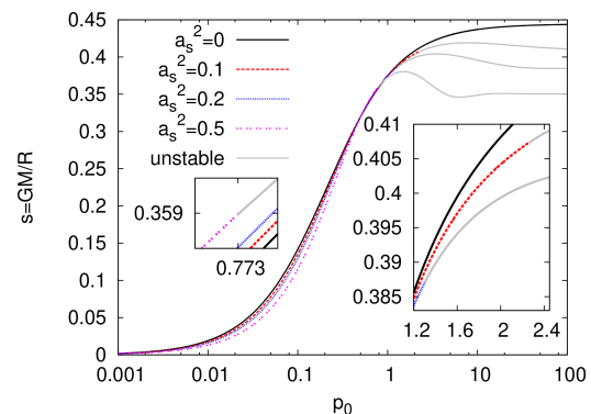
Refer to caption
Figure 7: The compactness s=GM/R𝑠𝐺𝑀𝑅s=GM/R plotted versus p0=P0/ρ0subscript𝑝0subscript𝑃0subscript𝜌0p_{0}=P_{0}/\rho_{0} for constant-density stars in Brans-Dicke theory, for various values of a02superscriptsubscript𝑎02a_{0}^{2}.

Equation (137) describes how the compactness depends on p0subscript𝑝0p_{0} in GR. In order to find how scalar-matter couplings modify this behaviour, it is necessary to solve the equations of stellar structure to first order in a02superscriptsubscript𝑎02a_{0}^{2}, and calculate s(1)subscript𝑠1s_{(1)}.

Figure 7 plots the compactness vs p0subscript𝑝0p_{0} in Brans-Dicke theory, for various values of the Brans-Dicke coupling a0=assubscript𝑎0subscript𝑎𝑠a_{0}=a_{s}. Notice that the compactness eventually stops growing with p0subscript𝑝0p_{0}, approaching instead an asymptotic value as p0subscript𝑝0p_{0}\to\infty. In GR, this asymptotic value is GM/R=4/9𝐺𝑀𝑅49GM/R=4/9, which is the maximum allowed by Buchdahl’s theorem. As a0subscript𝑎0a_{0} increases, this asymptotic value decreases. This is consistent with the results of [40].

5.3 Perturbative solutions: next-to-leading corrections

In this section, 𝒪(a02)𝒪superscriptsubscript𝑎02\mathcal{O}(a_{0}^{2}) corrections are calculated. The defining equation for U𝑈U is p(U)=0𝑝𝑈0p(U)=0. Expanding it in powers of a02superscriptsubscript𝑎02a_{0}^{2} yields

U(1)=12(1+p0)2(1+3p0)2p(1)(U(0)).subscript𝑈112superscript1subscript𝑝02superscript13subscript𝑝02subscript𝑝1subscript𝑈0U_{(1)}=\frac{12(1+p_{0})^{2}}{(1+3p_{0})^{2}}\;p_{(1)}(U_{(0)})\,. (171)

Solving equations (126) – (128) perturbatively in a02superscriptsubscript𝑎02a_{0}^{2} yields

μ(1)(u)subscript𝜇1𝑢\displaystyle\mu_{(1)}(u) =\displaystyle= 1u0udu^u^[φ(0)(1+bsφ(0)2)+u^(1u^/3)(φ˙(0))2],1𝑢superscriptsubscript0𝑢d^𝑢^𝑢delimited-[]subscript𝜑01subscript𝑏𝑠subscript𝜑02^𝑢1^𝑢3superscriptsubscript˙𝜑02\displaystyle\frac{1}{\sqrt{u}}\int_{0}^{u}{\hbox{d}}\hat{u}\sqrt{\hat{u}}\left[\varphi_{(0)}\left(1+\frac{b_{s}\varphi_{(0)}}{2}\right)+\hat{u}(1-\hat{u}/3)(\dot{\varphi}_{(0)})^{2}\right]\,, (172)
p1(u)subscript𝑝1𝑢\displaystyle p_{1}(u) =\displaystyle= 2(1+p0)φ(0)(1+bsφ(0)/2)(1+3p0)1u/33(1+p0)21subscript𝑝0subscript𝜑01subscript𝑏𝑠subscript𝜑0213subscript𝑝01𝑢331subscript𝑝0\displaystyle\frac{2(1+p_{0})\varphi_{(0)}\left(1+{b_{s}\varphi_{(0)}}/{2}\right)}{(1+3p_{0})\sqrt{1-u/3}-3(1+p_{0})} (173)
+2(1+p0)μ(1)(u)1u/3(1+p0)(32u)1u/3(1+3p0)((1+3p0)1u/33(1+p0))221subscript𝑝0subscript𝜇1𝑢1𝑢31subscript𝑝032𝑢1𝑢313subscript𝑝0superscript13subscript𝑝01𝑢331subscript𝑝02\displaystyle+\frac{2(1+p_{0})\mu_{(1)}(u)}{\sqrt{1-u/3}}\cdot\frac{(1+p_{0})(3-2u)\sqrt{1-u/3}-(1+3p_{0})}{((1+3p_{0})\sqrt{1-u/3}-3(1+p_{0}))^{2}}
+2(1+p0)1u/36((1+3p0)1u/33(1+p0))20udu^(1u^/3)3/2J(u^),21subscript𝑝01𝑢36superscript13subscript𝑝01𝑢331subscript𝑝02superscriptsubscript0𝑢d^𝑢superscript1^𝑢332𝐽^𝑢\displaystyle+\frac{2(1+p_{0})\sqrt{1-u/3}}{6((1+3p_{0})\sqrt{1-u/3}-3(1+p_{0}))^{2}}\int_{0}^{u}\frac{{\hbox{d}}\hat{u}}{(1-\hat{u}/3)^{3/2}}\;J(\hat{u})\,,

where the function J(u)𝐽𝑢J(u) appearing in equation (173) is given by

J(u)𝐽𝑢\displaystyle J(u) =\displaystyle= 2[6(1+3p0)1u/3(1+p0)(2u29u+18)]u(1u/3)(φ˙(0))22delimited-[]613subscript𝑝01𝑢31subscript𝑝02superscript𝑢29𝑢18𝑢1𝑢3superscriptsubscript˙𝜑02\displaystyle 2\Bigl{[}6(1+3p_{0})\sqrt{1-u/3}-(1+p_{0})(2u^{2}-9u+18)\Bigr{]}u(1-u/3)(\dot{\varphi}_{(0)})^{2} (174)
(1+p0)(4u218u+9)φ(0)(1+bsφ(0)2).1subscript𝑝04superscript𝑢218𝑢9subscript𝜑01subscript𝑏𝑠subscript𝜑02\displaystyle-(1+p_{0})(4u^{2}-18u+9)\varphi_{(0)}\left(1+\frac{b_{s}\varphi_{(0)}}{2}\right)\,.

The perturbation to the scalar profile is similarly

φ(1)=Φ1ψ+Φ2ψ~.subscript𝜑1subscriptΦ1𝜓subscriptΦ2~𝜓\varphi_{(1)}=\Phi_{1}\psi+\Phi_{2}\tilde{\psi}\,. (175)

where the functions ψ𝜓\psi and ψ~~𝜓\tilde{\psi} are local Frobenius solutions of equation (158) (with parameters (159) – (160)) about z=0𝑧0z=0 with exponents 00 and 1212-\frac{1}{2}, respectively. They are given by

ψ𝜓\displaystyle\psi =\displaystyle= HeunG(11+3p0,32bs3p013p0+1;\displaystyle{\rm HeunG}\biggl{(}\frac{-1}{1+3p_{0}},\frac{3}{2}b_{s}\cdot\frac{3p_{0}-1}{3p_{0}+1}; (176)
32(118bs/3),32(1+18bs/3),32,32;z),\displaystyle\hphantom{{\rm HeunG}\biggl{(}}\frac{3}{2}(1-\sqrt{1-8b_{s}/3}),\frac{3}{2}(1+\sqrt{1-8b_{s}/3}),\frac{3}{2},\frac{3}{2};z\biggr{)}\,,
ψ~~𝜓\displaystyle\tilde{\psi} =\displaystyle= 1zHeunG(11+3p0,6bs(3p01)+16p04(1+3p0);\displaystyle\frac{1}{\sqrt{z}}\;{\rm HeunG}\biggl{(}\frac{-1}{1+3p_{0}},\frac{6b_{s}(3p_{0}-1)+1-6p_{0}}{4(1+3p_{0})}; (177)
1+3218bs/3,13218bs/3,12,32;z),\displaystyle\hphantom{\frac{1}{\sqrt{z}}{\rm HeunG}\biggl{(}}1+\frac{3}{2}\sqrt{1-8b_{s}/3},1-\frac{3}{2}\sqrt{1-8b_{s}/3},\frac{1}{2},\frac{3}{2};z\biggr{)}\,,

where z=(11u/3)/2𝑧11𝑢32z=(1-\sqrt{1-u/3})/2. The coefficients Φ1subscriptΦ1\Phi_{1} and Φ2subscriptΦ2\Phi_{2} are given by

Φ1subscriptΦ1\displaystyle\Phi_{1} =\displaystyle= 2880zψ~(Fp(1)+Gμ(1)+H)(12z)2[z(1z)]3/2[1+(1+3p0)z]dz,288superscriptsubscript0𝑧~𝜓𝐹subscript𝑝1𝐺subscript𝜇1𝐻superscript12𝑧2superscriptdelimited-[]𝑧1𝑧32delimited-[]113subscript𝑝0𝑧d𝑧\displaystyle 288\int_{0}^{z}\tilde{\psi}(Fp_{(1)}+G\mu_{(1)}+H)(1-2z)^{2}[z(1-z)]^{3/2}[1+(1+3p_{0})z]\,{\hbox{d}}z\,, (178)
Φ2subscriptΦ2\displaystyle\Phi_{2} =\displaystyle= 2880zψ(Fp(1)+Gμ(1)+H)(12z)2[z(1z)]3/2[1+(1+3p0)z]dz,288superscriptsubscript0𝑧𝜓𝐹subscript𝑝1𝐺subscript𝜇1𝐻superscript12𝑧2superscriptdelimited-[]𝑧1𝑧32delimited-[]113subscript𝑝0𝑧d𝑧\displaystyle-288\int_{0}^{z}\psi(Fp_{(1)}+G\mu_{(1)}+H)(1-2z)^{2}[z(1-z)]^{3/2}[1+(1+3p_{0})z]\,{\hbox{d}}z\,, (179)

where

F𝐹\displaystyle F =\displaystyle= 1+bsφ(0)+8z(1z)φ˙(0)32z(1z)(12z)2,1subscript𝑏𝑠subscript𝜑08𝑧1𝑧subscript˙𝜑032𝑧1𝑧superscript12𝑧2\displaystyle-\frac{1+b_{s}\varphi_{(0)}+8z(1-z)\dot{\varphi}_{(0)}}{32z(1-z)(1-2z)^{2}}\,, (180)
G𝐺\displaystyle G =\displaystyle= (4(1+3p0)z+13p0)(1+bsφ(0))48z(1z)(12z)4(1+(1+3p0)z)413subscript𝑝0𝑧13subscript𝑝01subscript𝑏𝑠subscript𝜑048𝑧1𝑧superscript12𝑧4113subscript𝑝0𝑧\displaystyle\frac{(4(1+3p_{0})z+1-3p_{0})(1+b_{s}\varphi_{(0)})}{48z(1-z)(1-2z)^{4}(1+(1+3p_{0})z)} (181)
[12(1+3p0)z36(1+7p0)z2+(9p05)z+1]φ˙(0)12z(1z)(12z)4(1+(1+3p0)z),delimited-[]1213subscript𝑝0superscript𝑧3617subscript𝑝0superscript𝑧29subscript𝑝05𝑧1subscript˙𝜑012𝑧1𝑧superscript12𝑧4113subscript𝑝0𝑧\displaystyle\qquad\qquad-\frac{[12(1+3p_{0})z^{3}-6(1+7p_{0})z^{2}+(9p_{0}-5)z+1]\dot{\varphi}_{(0)}}{12z(1-z)(1-2z)^{4}(1+(1+3p_{0})z)}\,,
H𝐻\displaystyle H =\displaystyle= (4(1+3p0)z+13p0)φ(0)(1+bsφ(0))(1+bsφ(0)/2)24z(1z)(12z)2(1+(1+3p0)z)413subscript𝑝0𝑧13subscript𝑝0subscript𝜑01subscript𝑏𝑠subscript𝜑01subscript𝑏𝑠subscript𝜑0224𝑧1𝑧superscript12𝑧2113subscript𝑝0𝑧\displaystyle\frac{(4(1+3p_{0})z+1-3p_{0})\varphi_{(0)}(1+b_{s}\varphi_{(0)})(1+b_{s}\varphi_{(0)}/2)}{24z(1-z)(1-2z)^{2}(1+(1+3p_{0})z)} (182)
+(2(1+3p0)z+1p0)φ(0)(1+bsφ(0)/2)φ˙(0)(12z)2(1+(1+3p0)z).213subscript𝑝0𝑧1subscript𝑝0subscript𝜑01subscript𝑏𝑠subscript𝜑02subscript˙𝜑0superscript12𝑧2113subscript𝑝0𝑧\displaystyle\qquad\qquad+\frac{(2(1+3p_{0})z+1-p_{0})\varphi_{(0)}(1+b_{s}\varphi_{(0)}/2)\dot{\varphi}_{(0)}}{(1-2z)^{2}(1+(1+3p_{0})z)}\,.
Refer to caption
Refer to caption
Refer to caption
Refer to caption
Figure 8: Comparison of μ𝜇\mu vs u𝑢u calculated perturbatively and numerically for an incompressible star in quasi-Brans/Dicke theory with a02=0.1superscriptsubscript𝑎020.1a_{0}^{2}=0.1 and bs=4subscript𝑏𝑠4b_{s}=4, p0=0.1subscript𝑝00.1p_{0}=0.1 (top left); bs=4subscript𝑏𝑠4b_{s}=4, p0=1subscript𝑝01p_{0}=1 (top right); bs=4subscript𝑏𝑠4b_{s}=-4, p0=0.1subscript𝑝00.1p_{0}=0.1 (bottom left); and bs=4subscript𝑏𝑠4b_{s}=-4, p0=1subscript𝑝01p_{0}=1 (bottom right). All curves terminate at the stellar exterior, u=U𝑢𝑈u=U.

The first-order corrections to the external parameters are given by

(1)subscript1\displaystyle\mathcal{F}_{(1)} =\displaystyle= φ(1)12e2LLφ˙(1)3(1+p0)22p0(1+2p0)L(1+bsφ(0))p(1)subscript𝜑112superscript𝑒2𝐿𝐿subscript˙𝜑13superscript1subscript𝑝022subscript𝑝012subscript𝑝0𝐿1subscript𝑏𝑠subscript𝜑0subscript𝑝1\displaystyle\varphi_{(1)}-12e^{2L}L\dot{\varphi}_{(1)}-\frac{3(1+p_{0})^{2}}{2p_{0}(1+2p_{0})}L(1+b_{s}\varphi_{(0)})p_{(1)} (183)
+36e2L(1+1+4p0+5p022p0(1+2p0)L)(p(1)φ˙(0)+48e2Lp0(1+2p0)(1+3p0)2(φ˙(0))3)36superscript𝑒2𝐿114subscript𝑝05superscriptsubscript𝑝022subscript𝑝012subscript𝑝0𝐿subscript𝑝1subscript˙𝜑048superscript𝑒2𝐿subscript𝑝012subscript𝑝0superscript13subscript𝑝02superscriptsubscript˙𝜑03\displaystyle+36e^{2L}\left(1+\frac{1+4p_{0}+5p_{0}^{2}}{2p_{0}(1+2p_{0})}L\right)\left(p_{(1)}\dot{\varphi}_{(0)}+48e^{2L}\frac{p_{0}(1+2p_{0})}{(1+3p_{0})^{2}}(\dot{\varphi}_{(0)})^{3}\right)
+12(1+(1+3p0)22p0(1+2p0)L)φ˙(0)μ(1),121superscript13subscript𝑝022subscript𝑝012subscript𝑝0𝐿subscript˙𝜑0subscript𝜇1\displaystyle+12\left(1+\frac{(1+3p_{0})^{2}}{2p_{0}(1+2p_{0})}L\right)\dot{\varphi}_{(0)}\mu_{(1)}\,,
𝒜(1)subscript𝒜1\displaystyle\mathcal{A}_{(1)} =\displaystyle= 12e2Lφ˙(1)+3(1+p0)22p0(1+2p0)(1+bsφ(0))p(1)6(1+3p0)2p0(1+2p0)φ˙(0)μ(1)12superscript𝑒2𝐿subscript˙𝜑13superscript1subscript𝑝022subscript𝑝012subscript𝑝01subscript𝑏𝑠subscript𝜑0subscript𝑝16superscript13subscript𝑝02subscript𝑝012subscript𝑝0subscript˙𝜑0subscript𝜇1\displaystyle 12e^{2L}\dot{\varphi}_{(1)}+\frac{3(1+p_{0})^{2}}{2p_{0}(1+2p_{0})}(1+b_{s}\varphi_{(0)})p_{(1)}-6\frac{(1+3p_{0})^{2}}{p_{0}(1+2p_{0})}\dot{\varphi}_{(0)}\mu_{(1)} (184)
1728e4Lp0(1+2p0)(1+3p0)2(φ˙(0))318e2L(5p02+4p0+1)p0(1+2p0)φ˙(0)p(1),1728superscript𝑒4𝐿subscript𝑝012subscript𝑝0superscript13subscript𝑝02superscriptsubscript˙𝜑0318superscript𝑒2𝐿5superscriptsubscript𝑝024subscript𝑝01subscript𝑝012subscript𝑝0subscript˙𝜑0subscript𝑝1\displaystyle-1728e^{4L}\frac{p_{0}(1+2p_{0})}{(1+3p_{0})^{2}}(\dot{\varphi}_{(0)})^{3}-18e^{2L}\frac{(5p_{0}^{2}+4p_{0}+1)}{p_{0}(1+2p_{0})}\dot{\varphi}_{(0)}p_{(1)}\,,
s(1)subscript𝑠1\displaystyle s_{(1)} =\displaystyle= μ(1)+2e2Lp(1)144Lp0(1+2p0)(1+3p0)2e4L(φ˙(0))2,subscript𝜇12superscript𝑒2𝐿subscript𝑝1144𝐿subscript𝑝012subscript𝑝0superscript13subscript𝑝02superscript𝑒4𝐿superscriptsubscript˙𝜑02\displaystyle\mu_{(1)}+2e^{2L}p_{(1)}-144L\frac{p_{0}(1+2p_{0})}{(1+3p_{0})^{2}}e^{4L}(\dot{\varphi}_{(0)})^{2}\,, (185)
(1)subscript1\displaystyle\mathcal{M}_{(1)} =\displaystyle= 24(1+p0)3p0(1+2p0)(1+3p0)2p(1)+123p0(1+2p0)1+p0μ(1)241subscript𝑝03subscript𝑝012subscript𝑝0superscript13subscript𝑝02subscript𝑝1123subscript𝑝012subscript𝑝01subscript𝑝0subscript𝜇1\displaystyle\frac{24(1+p_{0})\sqrt{3p_{0}(1+2p_{0})}}{(1+3p_{0})^{2}}p_{(1)}+\frac{12\sqrt{3p_{0}(1+2p_{0})}}{1+p_{0}}\mu_{(1)} (186)
30U(0)𝑑uu1u/3[φ(0)(1+bsφ(0)/2)+2u(1u/3)(φ˙(0))2],3superscriptsubscript0subscript𝑈0differential-d𝑢𝑢1𝑢3delimited-[]subscript𝜑01subscript𝑏𝑠subscript𝜑022𝑢1𝑢3superscriptsubscript˙𝜑02\displaystyle-3\int_{0}^{U_{(0)}}du\sqrt{\frac{u}{1-u/3}}[\varphi_{(0)}(1+b_{s}\varphi_{(0)}/2)+2u(1-u/3)(\dot{\varphi}_{(0)})^{2}]\,,

where L=log(1+p0)log(1+3p0)𝐿1subscript𝑝013subscript𝑝0L=\log(1+p_{0})-\log(1+3p_{0}), and the profiles are all to be evaluated at U(0)subscript𝑈0U_{(0)}.

If bs0subscript𝑏𝑠0b_{s}\neq 0, then the relation aA=logM/ϕsubscript𝑎𝐴𝑀subscriptitalic-ϕa_{{\scriptscriptstyle A}}=\partial\log M/\partial\phi_{\infty} [2] can be used to simplify (1)subscript1\mathcal{M}_{(1)}:

(1)subscript1\displaystyle\mathcal{M}_{(1)} =\displaystyle= 932bsarccos(1+p01+3p0)3p0(1+2p0)(41p02+34p0+9)bs(1+p0)(1+3p0)2932subscript𝑏𝑠1subscript𝑝013subscript𝑝03subscript𝑝012subscript𝑝041superscriptsubscript𝑝0234subscript𝑝09subscript𝑏𝑠1subscript𝑝0superscript13subscript𝑝02\displaystyle\frac{9\sqrt{3}}{2b_{s}}\arccos\left(\frac{1+p_{0}}{1+3p_{0}}\right)-\frac{\sqrt{3p_{0}(1+2p_{0})}(41p_{0}^{2}+34p_{0}+9)}{b_{s}(1+p_{0})(1+3p_{0})^{2}} (187)
96(1+p0)3p03(1+2p0)3bs(1+3p0)4φ˙(0)(1+bsφ(0))+83p0(1+2p0)1+p0μ(1)961subscript𝑝03superscriptsubscript𝑝03superscript12subscript𝑝03subscript𝑏𝑠superscript13subscript𝑝04subscript˙𝜑01subscript𝑏𝑠subscript𝜑083subscript𝑝012subscript𝑝01subscript𝑝0subscript𝜇1\displaystyle-\frac{96(1+p_{0})\sqrt{3p_{0}^{3}(1+2p_{0})^{3}}}{b_{s}(1+3p_{0})^{4}}\;\dot{\varphi}_{(0)}(1+b_{s}\varphi_{(0)})+\frac{8\sqrt{3p_{0}(1+2p_{0})}}{1+p_{0}}\;\mu_{(1)}
+24(1+p0)3p0(1+2p0)(1+3p0)2p(1).241subscript𝑝03subscript𝑝012subscript𝑝0superscript13subscript𝑝02subscript𝑝1\displaystyle+\frac{24(1+p_{0})\sqrt{3p_{0}(1+2p_{0})}}{(1+3p_{0})^{2}}\;p_{(1)}\,.
Refer to caption
Refer to caption
Refer to caption
Refer to caption
Figure 9: Comparison of p𝑝p vs u𝑢u calculated perturbatively and numerically for an incompressible star in quasi-Brans/Dicke theory with a02=0.1superscriptsubscript𝑎020.1a_{0}^{2}=0.1 and bs=4subscript𝑏𝑠4b_{s}=4, p0=0.1subscript𝑝00.1p_{0}=0.1 (top left); bs=4subscript𝑏𝑠4b_{s}=4, p0=1subscript𝑝01p_{0}=1 (top right); bs=4subscript𝑏𝑠4b_{s}=-4, p0=0.1subscript𝑝00.1p_{0}=0.1 (bottom left); and bs=4subscript𝑏𝑠4b_{s}=-4, p0=1subscript𝑝01p_{0}=1 (bottom right). All curves terminate at the stellar exterior, u=U𝑢𝑈u=U.

5.4 Comparing perturbative solutions with numerics

Part of the utility of analyzing the incompressible star in such detail is that such explicit expressions for the perturbative solutions allow a detailed comparison with direct numerical integrations. This helps indicate the domain of validity of the perturbative results.

First, we look at the profiles for the physical variables μ(u)𝜇𝑢\mu(u), p(u)𝑝𝑢p(u), and φ(u)𝜑𝑢\varphi(u) across the interior of the star. The quantities μ𝜇\mu, p𝑝p and φ𝜑\varphi are respectively plotted versus u𝑢u in Figures (8), (9) and (10), for a02=0.1superscriptsubscript𝑎020.1a_{0}^{2}=0.1 and several choices for bssubscript𝑏𝑠b_{s}, and p0subscript𝑝0p_{0}. The line labelled “Zeroth Order” plots the zeroeth-order result, e.g. μ(0)subscript𝜇0\mu_{(0)}, while the line labelled “First Order” includes also the first correction, e.g. μ(0)+a02μ(1)subscript𝜇0superscriptsubscript𝑎02subscript𝜇1\mu_{(0)}+a_{0}^{2}\mu_{(1)}. Notice that the curves all lie close to one other for small u𝑢u, but begin to separate at the stellar exterior, uU𝑢𝑈u\to U. Furthermore, the separation is largest for the more relativistic stars, for which p0subscript𝑝0p_{0} is larger. However in all cases displayed the perturbative results capture the full numerics quite well throughout the entire star, with the strongest deviations happening for φ(u)𝜑𝑢\varphi(u) when bs<0subscript𝑏𝑠0b_{s}<0.

Refer to caption
Refer to caption
Refer to caption
Refer to caption
Figure 10: Comparison of φ𝜑\varphi vs u𝑢u calculated perturbatively and numerically for an incompressible star in quasi-Brans/Dicke theory with a02=0.1superscriptsubscript𝑎020.1a_{0}^{2}=0.1 and bs=4subscript𝑏𝑠4b_{s}=4, p0=0.1subscript𝑝00.1p_{0}=0.1 (top left); bs=4subscript𝑏𝑠4b_{s}=4, p0=1subscript𝑝01p_{0}=1 (top right); bs=4subscript𝑏𝑠4b_{s}=-4, p0=0.1subscript𝑝00.1p_{0}=0.1 (bottom left); and bs=4subscript𝑏𝑠4b_{s}=-4, p0=1subscript𝑝01p_{0}=1 (bottom right). All curves terminate at the stellar exterior, u=U𝑢𝑈u=U.

Of more practical interest is a similar comparison of the accuracy of the perturbative expressions for plots that directly relate observable quantities to one another, such as plots of aAsubscript𝑎𝐴a_{\scriptscriptstyle A} vs s𝑠s. Examples of these are given in figures (11), which give s𝑠s, 𝒜=aA/a0𝒜subscript𝑎𝐴subscript𝑎0\mathcal{A}=a_{\scriptscriptstyle A}/a_{0}, =(ϕϕ0)/a0subscriptitalic-ϕsubscriptitalic-ϕ0subscript𝑎0\mathcal{F}=(\phi_{\infty}-\phi_{0})/a_{0} and \mathcal{M} as functions of the central pressure, p0=P0/ρ0subscript𝑝0subscript𝑃0subscript𝜌0p_{0}=P_{0}/\rho_{0} for the special case of Brans-Dicke theory (bs=0subscript𝑏𝑠0b_{s}=0) with a02=as2=0.1superscriptsubscript𝑎02superscriptsubscript𝑎𝑠20.1a_{0}^{2}=a_{s}^{2}=0.1. These again show good agreement between perturbative and numerical calculations, with the biggest deviations arising in the most relativistic settings (largest p0subscript𝑝0p_{0}).

Refer to caption
Refer to caption
Refer to caption
Refer to caption
Figure 11: Comparison of physical quantities as functions of central pressure, p0=P0/ρ0subscript𝑝0subscript𝑃0subscript𝜌0p_{0}=P_{0}/\rho_{0}, calculated perturbatively and numerically for an incompressible star in Brans-Dicke theory (bs=0subscript𝑏𝑠0b_{s}=0) with as2=0.1superscriptsubscript𝑎𝑠20.1a_{s}^{2}=0.1. The plots show compactness, s𝑠s (top left); external coupling, 𝒜=aA/as=Q/Mas𝒜subscript𝑎𝐴subscript𝑎𝑠𝑄𝑀subscript𝑎𝑠\mathcal{A}=a_{\scriptscriptstyle A}/a_{s}=Q/Ma_{s}, (top right); =(ϕϕ0)/assubscriptitalic-ϕsubscriptitalic-ϕ0subscript𝑎𝑠\mathcal{F}=(\phi_{\infty}-\phi_{0})/a_{s} (bottom left); and \mathcal{M} (bottom right).

6 Conclusions

In this paper we set up the equations of stellar structure, with the stellar interior modeled as a spherically symmetric, static fluid, and with gravity described by a scalar-tensor theory with a single light scalar coupling to matter only through its coupling to a Jordan frame metric. For practical reasons, and for the purposes of making contact with earlier workers, we focus on the special case where the scalar-matter coupling function does not vary strongly with the field, a(ϕ)as+bsϕsimilar-to-or-equals𝑎italic-ϕsubscript𝑎𝑠subscript𝑏𝑠italic-ϕa(\phi)\simeq a_{s}+b_{s}\phi.

We seek solutions to these equations, for a variety of equations of state, in the special case where the scalar-matter coupling at the stellar center is small, a02=a2(ϕ0)1subscriptsuperscript𝑎20superscript𝑎2subscriptitalic-ϕ0much-less-than1a^{2}_{0}=a^{2}(\phi_{0})\ll 1. We obtain solutions as perturbations to those of General Relativity. By comparing these solutions with explicit numerical integration we verify that the perturbative approximation works well throughout most of the star.

These perturbative solutions have the merit of being very simple to integrate numerically, and of allowing analytic solutions for some choices of equation of state. This is very convenient for efficiently exploring different choices for the scalar properties, and scalar-matter couplings.

We use these solutions to compute the form of the observable relations that are imposed among the external properties of the stars by the condition that they match continuously to the stellar interior. There are two such relations among the four external variables, M𝑀M, R𝑅R, Q𝑄Q and ϕsubscriptitalic-ϕ\phi_{\infty}, and our semi-analytic approach allows a simple exposition of how these relations depend on scalar properties. These properties ultimately underly any tests of scalar-tensor theories using astrophysical systems, such as binary pulsars.

Finally, these methods are applied to the illustrative case of an incompressible star, for which the density is constant. In this case the solutions generated by the a0subscript𝑎0a_{0} expansion may be found analytically, making the comparisons with numerical results particularly simple. Again we find that the perturbative expressions agree well with the solutions obtained by numerical integration.

Acknowledgements

We thank Nemanja Kaloper and Maxim Pospelov for useful discussions. This research was supported in part by funds from the Natural Sciences and Engineering Research Council (NSERC) of Canada. Research at the Perimeter Institute is supported in part by the Government of Canada through Industry Canada, and by the Province of Ontario through the Ministry of Research and Information (MRI).

Appendix A Expansions for large bssubscript𝑏𝑠b_{s}

This appendix evaluates the large-bssubscript𝑏𝑠b_{s} expansion for the properties of incompressible stars.

The coefficients crsubscript𝑐𝑟c_{r} of the power series (162) can be written explicitly as

cr=i=0rai(r)bsi,subscript𝑐𝑟superscriptsubscript𝑖0𝑟superscriptsubscript𝑎𝑖𝑟superscriptsubscript𝑏𝑠𝑖c_{r}=\sum_{i=0}^{r}a_{i}^{(r)}b_{s}^{i}\,, (188)

where ai(r)superscriptsubscript𝑎𝑖𝑟a_{i}^{(r)} is a polynomial in p0subscript𝑝0p_{0} of degree r𝑟r. It follows from equation (5.2) that ar(r)superscriptsubscript𝑎𝑟𝑟a_{r}^{(r)} satisfy a two-term recurrence relation, which can be solved explicitly, giving

ar(r)=[6(13p0)]r(2r+1)!.superscriptsubscript𝑎𝑟𝑟superscriptdelimited-[]613subscript𝑝0𝑟2𝑟1a_{r}^{(r)}=\frac{[6(1-3p_{0})]^{r}}{(2r+1)!}\,. (189)

The coefficients a0(r)subscriptsuperscript𝑎𝑟0a^{(r)}_{0} vanish for r1𝑟1r\geq 1, and the remaining coefficients are given by

ark(r)=r![6(13p0)]r2k(2r+1)!(rk1)!j=02k1Pk,j(p0)rj,(k1,rk1)subscriptsuperscript𝑎𝑟𝑟𝑘𝑟superscriptdelimited-[]613subscript𝑝0𝑟2𝑘2𝑟1𝑟𝑘1superscriptsubscript𝑗02𝑘1subscript𝑃𝑘𝑗subscript𝑝0superscript𝑟𝑗formulae-sequence𝑘1𝑟𝑘1a^{(r)}_{r-k}=\frac{r!\cdot[6(1-3p_{0})]^{r-2k}}{(2r+1)!(r-k-1)!}\sum_{j=0}^{2k-1}P_{k,j}(p_{0})r^{j}\,,\qquad(k\geq 1,\ r-k\geq 1) (190)

where Pk,jsubscript𝑃𝑘𝑗P_{k,j} is a polynomial of degree 2k2𝑘2k with rational coefficients. The first of these polynomials are given by

P1,0(p0)subscript𝑃10subscript𝑝0\displaystyle P_{1,0}(p_{0}) =\displaystyle= 2(63p0218p0+7),263superscriptsubscript𝑝0218subscript𝑝07\displaystyle 2(63p_{0}^{2}-18p_{0}+7)\,, (191)
P1,1(p0)subscript𝑃11subscript𝑝0\displaystyle P_{1,1}(p_{0}) =\displaystyle= 8(9p02+9p0+4),89superscriptsubscript𝑝029subscript𝑝04\displaystyle 8(9p_{0}^{2}+9p_{0}+4)\,, (192)
P2,0(p0)subscript𝑃20subscript𝑝0\displaystyle P_{2,0}(p_{0}) =\displaystyle= 65(3321p04+2916p03+6426p02+4644p0+679),653321superscriptsubscript𝑝042916superscriptsubscript𝑝036426superscriptsubscript𝑝024644subscript𝑝0679\displaystyle\textstyle{\frac{6}{5}}(-3321p_{0}^{4}+2916p_{0}^{3}+6426p_{0}^{2}+4644p_{0}+679)\,, (193)
P2,1(p0)subscript𝑃21subscript𝑝0\displaystyle P_{2,1}(p_{0}) =\displaystyle= 25(5913p0421708p03+29502p02+17028p0+2593),255913superscriptsubscript𝑝0421708superscriptsubscript𝑝0329502superscriptsubscript𝑝0217028subscript𝑝02593\displaystyle\textstyle{\frac{2}{5}}(5913p_{0}^{4}-21708p_{0}^{3}+29502p_{0}^{2}+17028p_{0}+2593)\,, (194)
P2,2(p0)subscript𝑃22subscript𝑝0\displaystyle P_{2,2}(p_{0}) =\displaystyle= 485(729p04729p031989p021251p0176),485729superscriptsubscript𝑝04729superscriptsubscript𝑝031989superscriptsubscript𝑝021251subscript𝑝0176\displaystyle\textstyle{\frac{48}{5}}(729p_{0}^{4}-729p_{0}^{3}-1989p_{0}^{2}-1251p_{0}-176)\,, (195)
P2,3(p0)subscript𝑃23subscript𝑝0\displaystyle P_{2,3}(p_{0}) =\displaystyle= 32(9p02+9p0+4)2,32superscript9superscriptsubscript𝑝029subscript𝑝042\displaystyle 32(9p_{0}^{2}+9p_{0}+4)^{2}\,, (196)

and the higher ones can be computed from the relation

r!12(rl1)!i=02l1Pl,i(p0)ri=𝑟12𝑟𝑙1superscriptsubscript𝑖02𝑙1subscript𝑃𝑙𝑖subscript𝑝0superscript𝑟𝑖absent\displaystyle\displaystyle\frac{r!}{12(r-l-1)!}\sum_{i=0}^{2l-1}P_{l,i}(p_{0})r^{i}=\qquad\qquad
=24j=lr1(2j+1)(j+2)(1+3p0)(13p0)2j!(jl)!i=02l5Pl2,i(p0)(j1)i+1absent24superscriptsubscript𝑗𝑙𝑟12𝑗1𝑗213subscript𝑝0superscript13subscript𝑝02𝑗𝑗𝑙superscriptsubscript𝑖02𝑙5subscript𝑃𝑙2𝑖subscript𝑝0superscript𝑗1𝑖1\displaystyle\displaystyle\qquad\qquad=24\sum_{j=l}^{r-1}\frac{(2j+1)(j+2)(1+3p_{0})(1-3p_{0})^{2}j!}{(j-l)!}\sum_{i=0}^{2l-5}P_{l-2,i}(p_{0})(j-1)^{i+1}
+j=lr1(19p06jp0)(13p0)jj!(jl)!i=02l3Pl1,i(p0)jisuperscriptsubscript𝑗𝑙𝑟119subscript𝑝06𝑗subscript𝑝013subscript𝑝0𝑗𝑗𝑗𝑙superscriptsubscript𝑖02𝑙3subscript𝑃𝑙1𝑖subscript𝑝0superscript𝑗𝑖\displaystyle\displaystyle\qquad\qquad+\sum_{j=l}^{r-1}\frac{(1-9p_{0}-6jp_{0})(1-3p_{0})jj!}{(j-l)!}\sum_{i=0}^{2l-3}P_{l-1,i}(p_{0})j^{i}
+4j=l+1r1(2j+1)(1+3p0)j!(jl1)!i=02l3Pl1,i(p0)(j1)i,4superscriptsubscript𝑗𝑙1𝑟12𝑗113subscript𝑝0𝑗𝑗𝑙1superscriptsubscript𝑖02𝑙3subscript𝑃𝑙1𝑖subscript𝑝0superscript𝑗1𝑖\displaystyle\displaystyle\qquad\qquad+4\sum_{j=l+1}^{r-1}\frac{(2j+1)(1+3p_{0})j!}{(j-l-1)!}\sum_{i=0}^{2l-3}P_{l-1,i}(p_{0})(j-1)^{i}\,, (197)

which holds for l3𝑙3l\geq 3 and rl+1𝑟𝑙1r\geq l+1.

From the identities [67]

k=0n(1)k(nk)(k+a)nsuperscriptsubscript𝑘0𝑛superscript1𝑘binomial𝑛𝑘superscript𝑘𝑎𝑛\displaystyle\sum_{k=0}^{n}(-1)^{k}\binom{n}{k}(k+a)^{n} =\displaystyle= (1)nn!,(n0,a)superscript1𝑛𝑛formulae-sequence𝑛0𝑎\displaystyle(-1)^{n}n!\,,\qquad(n\geq 0,\ a\in\mathbb{R}) (198)
k=0N(1)k(Nk)(k+a)n1superscriptsubscript𝑘0𝑁superscript1𝑘binomial𝑁𝑘superscript𝑘𝑎𝑛1\displaystyle\sum_{k=0}^{N}(-1)^{k}\binom{N}{k}(k+a)^{n-1} =\displaystyle= 0,(Nn1,a)\displaystyle 0\,,\qquad(N\geq n\geq 1,\ a\in\mathbb{R}) (199)

it follows that

Pk,2k1(p0)=[8(9p02+9p0+4)]kk!.(k1)P_{k,2k-1}(p_{0})=\frac{[8(9p_{0}^{2}+9p_{0}+4)]^{k}}{k!}\,.\qquad(k\geq 1) (200)

Write

Pk,j(p0)=l=02kqk,j(l)p0l.subscript𝑃𝑘𝑗subscript𝑝0superscriptsubscript𝑙02𝑘superscriptsubscript𝑞𝑘𝑗𝑙superscriptsubscript𝑝0𝑙P_{k,j}(p_{0})=\sum_{l=0}^{2k}q_{k,j}^{(l)}p_{0}^{l}\,. (201)

By means of telescopic summation, the identity (197) can be used to derive recurrence relations for the coefficients qk,j(l)superscriptsubscript𝑞𝑘𝑗𝑙q_{k,j}^{(l)}. In general, these recurrence relations are very complicated, but for l=2k𝑙2𝑘l=2k, they are particularly simple:

(k+1)qk,0(2k)+i=12k1qk,i(2k)𝑘1superscriptsubscript𝑞𝑘02𝑘superscriptsubscript𝑖12𝑘1superscriptsubscript𝑞𝑘𝑖2𝑘\displaystyle(k+1)q_{k,0}^{(2k)}+\sum_{i=1}^{2k-1}q_{k,i}^{(2k)} =\displaystyle= 0,0\displaystyle 0\,, (202)
(k+2)qk,1(2k)+i=22k1(i+1)qk,i(2k)𝑘2superscriptsubscript𝑞𝑘12𝑘superscriptsubscript𝑖22𝑘1𝑖1superscriptsubscript𝑞𝑘𝑖2𝑘\displaystyle(k+2)q_{k,1}^{(2k)}+\sum_{i=2}^{2k-1}(i+1)q_{k,i}^{(2k)} =\displaystyle= 324qk1,0(2k2),324superscriptsubscript𝑞𝑘102𝑘2\displaystyle 324q_{k-1,0}^{(2k-2)}\,, (203)
(k+j+1)qk,j(2k)+i=j+12k1(i+1j)qk,i(2k)𝑘𝑗1superscriptsubscript𝑞𝑘𝑗2𝑘superscriptsubscript𝑖𝑗12𝑘1binomial𝑖1𝑗superscriptsubscript𝑞𝑘𝑖2𝑘\displaystyle(k+j+1)q_{k,j}^{(2k)}+\sum_{i=j+1}^{2k-1}\binom{i+1}{j}q_{k,i}^{(2k)} =\displaystyle= 216qk1,j2(2k2)+324qk1,j1(2k2),216superscriptsubscript𝑞𝑘1𝑗22𝑘2324superscriptsubscript𝑞𝑘1𝑗12𝑘2\displaystyle 216q_{k-1,j-2}^{(2k-2)}+324q_{k-1,j-1}^{(2k-2)}\,, (204)

where k2𝑘2k\geq 2 and 2j2k22𝑗2𝑘22\leq j\leq 2k-2.

Now, φ(0)subscript𝜑0\varphi_{(0)} can be expanded in the form

φ(0)(z)subscript𝜑0𝑧\displaystyle\varphi_{(0)}(z) =\displaystyle= 1bs[(a1(1)bs+a0(1))z+(a2(2)bs2+a1(2)bs+a0(2))z2\displaystyle\frac{1}{b_{s}}\biggl{[}(a_{1}^{(1)}b_{s}+a_{0}^{(1)})z+(a_{2}^{(2)}b_{s}^{2}+a_{1}^{(2)}b_{s}+a_{0}^{(2)})z^{2} (205)
+(a3(3)bs3+a2(3)bs2+a1(3)bs+a0(3))z3+]\displaystyle\hphantom{\frac{1}{b_{s}}\biggl{[}}+(a_{3}^{(3)}b_{s}^{3}+a_{2}^{(3)}b_{s}^{2}+a_{1}^{(3)}b_{s}+a_{0}^{(3)})z^{3}+\ldots\ \biggr{]}
=\displaystyle= 1bs(a1(1)(bsz)+a2(2)(bsz)2+a3(3)(bsz)3+)1subscript𝑏𝑠superscriptsubscript𝑎11subscript𝑏𝑠𝑧superscriptsubscript𝑎22superscriptsubscript𝑏𝑠𝑧2superscriptsubscript𝑎33superscriptsubscript𝑏𝑠𝑧3\displaystyle\frac{1}{b_{s}}\biggl{(}a_{1}^{(1)}(b_{s}z)+a_{2}^{(2)}(b_{s}z)^{2}+a_{3}^{(3)}(b_{s}z)^{3}+\ldots\biggr{)}
+1bs2(a0(1)(bsz)+a1(2)(bsz)2+a2(3)(bsz)3+)+1superscriptsubscript𝑏𝑠2superscriptsubscript𝑎01subscript𝑏𝑠𝑧superscriptsubscript𝑎12superscriptsubscript𝑏𝑠𝑧2superscriptsubscript𝑎23superscriptsubscript𝑏𝑠𝑧3\displaystyle+\frac{1}{b_{s}^{2}}\biggl{(}a_{0}^{(1)}(b_{s}z)+a_{1}^{(2)}(b_{s}z)^{2}+a_{2}^{(3)}(b_{s}z)^{3}+\ldots\biggr{)}+\ldots
\displaystyle\equiv φ(0)(1)(bsz)bs+φ(0)(2)(bsz)bs2+.subscriptsuperscript𝜑10subscript𝑏𝑠𝑧subscript𝑏𝑠subscriptsuperscript𝜑20subscript𝑏𝑠𝑧superscriptsubscript𝑏𝑠2\displaystyle\frac{\varphi^{(1)}_{(0)}(b_{s}z)}{b_{s}}+\frac{\varphi^{(2)}_{(0)}(b_{s}z)}{b_{s}^{2}}+\ldots\,.

It follows from equations (189) and (190) that

φ(0)(1)(bsz)subscriptsuperscript𝜑10subscript𝑏𝑠𝑧\displaystyle\varphi^{(1)}_{(0)}(b_{s}z) =\displaystyle= sinhtt1,𝑡𝑡1\displaystyle\frac{\sinh\sqrt{t}}{\sqrt{t}}-1\,, (206)
φ(k+1)(0)(bsz)superscriptsubscript𝜑𝑘10subscript𝑏𝑠𝑧\displaystyle\varphi_{(k+1)}^{(0)}(b_{s}z) =\displaystyle= 1[6(13p0)]2kj=02k1Pk,j(p0)fk,j(t),(k1)1superscriptdelimited-[]613subscript𝑝02𝑘superscriptsubscript𝑗02𝑘1subscript𝑃𝑘𝑗subscript𝑝0subscript𝑓𝑘𝑗𝑡𝑘1\displaystyle\frac{1}{[6(1-3p_{0})]^{2k}}\sum_{j=0}^{2k-1}P_{k,j}(p_{0})f_{k,j}(t)\,,\qquad(k\geq 1) (207)

where

fk,j(t)subscript𝑓𝑘𝑗𝑡\displaystyle f_{k,j}(t) =\displaystyle= r=k+1r!trrj(2r+1)!(rk1)!superscriptsubscript𝑟𝑘1𝑟superscript𝑡𝑟superscript𝑟𝑗2𝑟1𝑟𝑘1\displaystyle\sum_{r=k+1}^{\infty}\frac{r!\cdot t^{r}r^{j}}{(2r+1)!(r-k-1)!} (208)
=\displaystyle= (tddt)j(it2)k+1jk+1(it),superscript𝑡𝑑𝑑𝑡𝑗superscript𝑖𝑡2𝑘1subscript𝑗𝑘1𝑖𝑡\displaystyle\left(t\frac{d}{dt}\right)^{j}\left(-\frac{i\sqrt{t}}{2}\right)^{k+1}j_{k+1}(i\sqrt{t})\,,

where

jn(x)=π2xJn+12(x)=(x)n(1xddx)nsinxxsubscript𝑗𝑛𝑥𝜋2𝑥subscript𝐽𝑛12𝑥superscript𝑥𝑛superscript1𝑥𝑑𝑑𝑥𝑛𝑥𝑥j_{n}(x)=\sqrt{\frac{\pi}{2x}}J_{n+\frac{1}{2}}(x)=(-x)^{n}\left(\frac{1}{x}\frac{d}{dx}\right)^{n}\frac{\sin x}{x} (209)

are the spherical Bessel functions, and t=6bs(13p0)z=3bs(13p0)(11u/3)𝑡6subscript𝑏𝑠13subscript𝑝0𝑧3subscript𝑏𝑠13subscript𝑝011𝑢3t=6b_{s}(1-3p_{0})z=3b_{s}(1-3p_{0})(1-\sqrt{1-u/3}).

The spherical Bessel functions satisfy the recursion relations

xjl1(x)+xjl+1(x)=(2l+1)jl(x),𝑥subscript𝑗𝑙1𝑥𝑥subscript𝑗𝑙1𝑥2𝑙1subscript𝑗𝑙𝑥\displaystyle xj_{l-1}(x)+xj_{l+1}(x)=(2l+1)j_{l}(x)\,,
ljl1(x)(l+1)jl+1(x)=(2l+1)jl(x).𝑙subscript𝑗𝑙1𝑥𝑙1subscript𝑗𝑙1𝑥2𝑙1superscriptsubscript𝑗𝑙𝑥\displaystyle lj_{l-1}(x)-(l+1)j_{l+1}(x)=(2l+1)j_{l}^{\prime}(x)\,. (210)

Therefore, the fk,jsubscript𝑓𝑘𝑗f_{k,j} satisfy the recursion relations

fk,1=fk+1,0+(k+1)fk,0,subscript𝑓𝑘1subscript𝑓𝑘10𝑘1subscript𝑓𝑘0\displaystyle f_{k,1}=f_{k+1,0}+(k+1)f_{k,0}\,,
tfk1,04fk+1,0=2(2k+3)fk,0.𝑡subscript𝑓𝑘104subscript𝑓𝑘1022𝑘3subscript𝑓𝑘0\displaystyle tf_{k-1,0}-4f_{k+1,0}=2(2k+3)f_{k,0}\,. (211)

The first of these relations can be used to write fk,jsubscript𝑓𝑘𝑗f_{k,j} explicitly in terms of fl,0subscript𝑓𝑙0f_{l,0}:

fk,j=fk+j,0+m=1j[~l1,,lm=1jm+1(k+l1)(k+lm)]fk+jm,0,subscript𝑓𝑘𝑗subscript𝑓𝑘𝑗0superscriptsubscript𝑚1𝑗delimited-[]superscriptsubscript~subscript𝑙1subscript𝑙𝑚1𝑗𝑚1𝑘subscript𝑙1𝑘subscript𝑙𝑚subscript𝑓𝑘𝑗𝑚0\displaystyle f_{k,j}=f_{k+j,0}+\sum_{m=1}^{j}\left[\tilde{\sum}_{l_{1},\ldots,l_{m}=1}^{j-m+1}(k+l_{1})\ldots(k+l_{m})\right]f_{k+j-m,0}\,, (212)

for j1𝑗1j\geq 1. The tilde on the sum means that all numerical factors which come from overcounting should be deleted. For example,

~l1,l2=12(k+l1)(k+l2)=(k+1)2+(k+1)(k+2)+(k+2)2.superscriptsubscript~subscript𝑙1subscript𝑙212𝑘subscript𝑙1𝑘subscript𝑙2superscript𝑘12𝑘1𝑘2superscript𝑘22\tilde{\sum}_{l_{1},l_{2}=1}^{2}(k+l_{1})(k+l_{2})=(k+1)^{2}+(k+1)(k+2)+(k+2)^{2}\,. (213)

Equations (135)-(136) then become

𝒜(0)subscript𝒜0\displaystyle\mathcal{A}_{(0)} =\displaystyle= 1+p0p0{12bs(coshTsinhTT)+k=1j=02k1Pk,j(p0)fk,j+1(T)bsk+1[6(13p0)]2k},1subscript𝑝0subscript𝑝012subscript𝑏𝑠𝑇𝑇𝑇superscriptsubscript𝑘1superscriptsubscript𝑗02𝑘1subscript𝑃𝑘𝑗subscript𝑝0subscript𝑓𝑘𝑗1𝑇superscriptsubscript𝑏𝑠𝑘1superscriptdelimited-[]613subscript𝑝02𝑘\displaystyle\frac{1+p_{0}}{p_{0}}\left\{\frac{1}{2b_{s}}\left(\cosh\sqrt{T}-\frac{\sinh\sqrt{T}}{\sqrt{T}}\right)+\sum_{k=1}^{\infty}\sum_{j=0}^{2k-1}\frac{P_{k,j}(p_{0})f_{k,j+1}(T)}{b_{s}^{k+1}[6(1-3p_{0})]^{2k}}\right\}\,, (214)
(0)subscript0\displaystyle\mathcal{F}_{(0)} =\displaystyle= 1bs([1+1+p02p0L]sinhTT1+p02p0LcoshT1)1subscript𝑏𝑠delimited-[]11subscript𝑝02subscript𝑝0𝐿𝑇𝑇1subscript𝑝02subscript𝑝0𝐿𝑇1\displaystyle\frac{1}{b_{s}}\left(\left[1+\frac{1+p_{0}}{2p_{0}}L\right]\frac{\sinh\sqrt{T}}{\sqrt{T}}-\frac{1+p_{0}}{2p_{0}}L\cosh\sqrt{T}-1\right) (215)
+k=1j=02k1(fk,j(T)1+p0p0Lfk,j+1(T))Pk,j(p0)bsk+1[6(13p0)]2k,superscriptsubscript𝑘1superscriptsubscript𝑗02𝑘1subscript𝑓𝑘𝑗𝑇1subscript𝑝0subscript𝑝0𝐿subscript𝑓𝑘𝑗1𝑇subscript𝑃𝑘𝑗subscript𝑝0superscriptsubscript𝑏𝑠𝑘1superscriptdelimited-[]613subscript𝑝02𝑘\displaystyle+\sum_{k=1}^{\infty}\sum_{j=0}^{2k-1}\left(f_{k,j}(T)-\frac{1+p_{0}}{p_{0}}Lf_{k,j+1}(T)\right)\frac{P_{k,j}(p_{0})}{b_{s}^{k+1}[6(1-3p_{0})]^{2k}}\,,

where T=6bsp0(13p0)/(1+3p0)𝑇6subscript𝑏𝑠subscript𝑝013subscript𝑝013subscript𝑝0T=6b_{s}p_{0}(1-3p_{0})/(1+3p_{0}) is the value of the variable t𝑡t corresponding to u=U𝑢𝑈u=U, and L=log(1+p0)log(1+3p0)𝐿1subscript𝑝013subscript𝑝0L=\log(1+p_{0})-\log(1+3p_{0}). If bs>0subscript𝑏𝑠0b_{s}>0, then T(642)bs0.34bs𝑇642subscript𝑏𝑠similar-to0.34subscript𝑏𝑠T\leq(6-4\sqrt{2})b_{s}\sim 0.34b_{s}. If bs<0subscript𝑏𝑠0b_{s}<0, then T(642)|bs|0.34|bs|𝑇642subscript𝑏𝑠similar-to0.34subscript𝑏𝑠T\geq-(6-4\sqrt{2})|b_{s}|\sim-0.34|b_{s}|. The above expressions (214) and (215) can be used to calculate the second constraint (100).

These perturbative solutions have a limited regime of applicability. They break down as bs0subscript𝑏𝑠0b_{s}\to 0, because the 1/bs1subscript𝑏𝑠1/b_{s} expansion fails. But they also break down at the onset of spontaneous scalarization.

References

  • [1] T. Chiba, T. Harada, and K. Nakao, Prog. Theor. Phys. Suppl. 128 (1997) 335.
  • [2] T. Damour and G. Esposito-Farèse, Class. and Quant. Grav. 9 (1992) 2093.
  • [3] Y. Fujii and K. Maeda, The Scalar-Tensor Theory of Gravitation, Cambridge University Press 2003.
  • [4] V. Faraoni, Cosmology in Scalar-Tensor Gravity, Kluwer Academic Publishers 2004.
  • [5] T. Singh and L. N. Rai, Gen. Rel. Grav. 15 (1983) 875.
  • [6] C. H. Brans, [arXiv:gr-qc/0506063].
  • [7] S. Weinberg, Phys. Rev. Lett.  29 (1972) 1698.
  • [8] C. P. Burgess, A. Maharana and F. Quevedo, arXiv:1005.1199 [hep-th].
  • [9] C. M. Will, Living Rev. Rel.  9 (2005) 3 [arXiv:gr-qc/0510072].
  • [10] G. Esposito-Farèse, AIP Conf. Proc.  736 (2004) 35 [arXiv:gr-qc/0409081].
  • [11] T. Damour and G. Esposito-Farese, Phys. Rev.  D 54 (1996) 1474 [arXiv:gr-qc/9602056]; T. Damour, arXiv:0704.0749 [gr-qc]; G. Esposito-Farèse, [arXiv:gr-qc/0402007].
  • [12] T. Damour and G. Esposito-Farese, Phys. Rev.  D 58 (1998) 042001 [arXiv:gr-qc/9803031].
  • [13] N. D. R. Bhat, M. Bailes and J. P. W. Verbiest, Phys. Rev.  D 77 (2008) 124017 [arXiv:0804.0956 [astro-ph]]; K. Lazaridis et al., Mon. Not. R. Astron. Soc. 400 (2009) 805 [arXiv:0908.0285 [astro-ph.GA]].
  • [14] S. DeDeo and D. Psaltis, Phys. Rev. Lett.  90 (2003) 141101 [arXiv:astro-ph/0302095] ; S. DeDeo and D. Psaltis, Bull. Am. Astron. Soc. 36 (2004) 944 [arXiv:astro-ph/0405067]; D. Psaltis, arXiv:0806.1531 [astro-ph].
  • [15] O. G. Benvenuto, L. G. Althaus, and D. F. Torres, Mon. Not. R. Astron. Soc. 305 (1999) 905.
  • [16] H. Sotani and K. D. Kokkotas, Phys. Rev.  D 70 (2004) 084026 [arXiv:gr-qc/0409066]; H. Sotani and K. D. Kokkotas, Phys. Rev.  D 71 (2005) 124038 [arXiv:gr-qc/0506060].
  • [17] D. Psaltis, Astrophys. J. 688 (2008) 1282 [arXiv:astro-ph/0501234].
  • [18] T. Damour and G. Esposito-Farèse, Phys. Rev. Lett. 70 (1993) 2220.
  • [19] H. A. Buchdahl, Phys. Rev. 116 (1959) 1027.
  • [20] S. Weinberg, Gravitation and Cosmology, John Wiley & Sons 1972.
  • [21] C. W. Misner, K. S. Thorne, and J. A. Wheeler, Gravitation, W. H. Freeman and Company 1973.
  • [22] C. Brans and R. H. Dicke, Phys. Rev. 124 (1961) 925; R. H. Dicke, Phys. Rev. 125 (1962) 2163; C. Brans, Phys. Rev. 125 (1962) 2194.
  • [23] P. G. Bergmann, Int. J. Theor. Phys. 1 (1968) 25; R. V. Wagoner, Phys. Rev. D 1 (1970) 3209; K. Nordtvedt, Astrophys. J. 161 (1970) 1059.
  • [24] T. Damour and A. M. Polyakov, Gen. Rel. Grav.  26 (1994) 1171 [arXiv:gr-qc/9411069]; Nucl. Phys.  B 423 (1994) 532 [arXiv:hep-th/9401069].
  • [25] A. Albrecht, C. P. Burgess, F. Ravndal and C. Skordis, Phys. Rev.  D 65 (2002) 123507 [arXiv:astro-ph/0107573]; K. Kainulainen and D. Sunhede, Phys. Rev.  D 73 (2006) 083510 [arXiv:astro-ph/0412609].
  • [26] D. F. Mota and J. D. Barrow, Phys. Lett. B581 (2004) 141 [arXiv:astro-ph/0306047].
  • [27] J. Khoury and A. Weltman, Phys. Rev. Lett.  93 (2004) 171104 [arXiv:astro-ph/0309300].
  • [28] K. A. Olive and M. Pospelov, Phys. Rev.  D 77 (2008) 043524 [arXiv:0709.3825 [hep-ph]].
  • [29] J.H. Taylor, Rev. Mod. Phys. 66 (1994) 711; E.S. Phinney and S.R. Kulkarni, Ann. Rev. Astron. Astrophys. 32 (1994) 591.
  • [30] I. H. Stairs, Living Rev. Rel.  6 (2003) 5 [arXiv:astro-ph/0307536]; R. P. Breton et al., AIP Conf. Proc.  983 (2008) 469.
  • [31] J. M. Weisberg and J. H. Taylor, ASP Conf. Ser.  328 (2005) 25 [arXiv:astro-ph/0407149].
  • [32] T. Harada, Prog. Theor. Phys.  98 (1997) 359 [arXiv:gr-qc/9706014]; T. Harada, Phys. Rev.  D 57 (1998) 4802 [arXiv:gr-qc/9801049].
  • [33] J. Novak, Phys. Rev. D 57 (1998) 4789; J. Novak, Phys. Rev.  D 58 (1998) 064019 [arXiv:gr-qc/9806022]; J. Novak and J. M. Ibáñez, Astrophys. J. 533 (2000) 392; M. Alcubierre, J. C. Degollado, D. Nunez, M. Ruiz and M. Salgado, Phys. Rev.  D 81 (2010) 124018 [arXiv:1003.4767 [gr-qc]].
  • [34] A. Salmona, Phys. Rev. 154 (1967) 1218.
  • [35] Y. Nutku Astrophys. J. 155 (1969) 999.
  • [36] G. S. Saakyan and M. A. Mnatsakanyan, Astrophysics 3 (1967) 311; G. S. Saakyan and M. A. Mnatsakanyan, Astrophysics 4 (1968) 567; R. M. Avakyan and M. A. Mnatsakanyan, Astrophysics 5 (1969) 169; G. S. Saakyan and M. A. Mnatsakanyan, Astrophysics 5 (1969) 555.
  • [37] T. Matsuda, Prog. Theor. Phys. 48 (1972) 341.
  • [38] K. Yokoi, Prog. Theor. Phys. 48 (1972) 1760.
  • [39] H. Heintzmann, W. Hillebrandt, M. F. El Eid, and E. R. Hilf, Z. Naturforsch. 29a (1974) 933.
  • [40] W. Hillebrandt and H. Heintzmann, Gen. Rel. Grav. 5 (1974) 663.
  • [41] V. I. Reizlin, Sov. J. Phys. 19 (1976) 1403.
  • [42] R. A. Saenz, Astrophys. J. 212 (1977) 816.
  • [43] W. F. Bruckman and E. Kazes, Phys. Rev. D 16 (1977) 261; W. F. Bruckman and E. Kazes, Phys. Rev. D 16 (1977) 269.
  • [44] A. Banerjee and D. Bhattacharya, J. Math. Phys. 20 (1979) 1908; A. Banerjee and N. O. Santos, Int. J. Theor. Phys. 20 (1981) 315.
  • [45] R. M. Avakyan, G. G. Arutyunyan, and V. V. Papoyan, Astrophysics 33 (1991) 338.
  • [46] H. W. Zaglauer, Astrophys. J. 393 (1992) 685.
  • [47] W. F. Bruckman and E. S. Velázquez, Gen. Rel. Grav. 25 (1993) 901.
  • [48] M. Salgado, D. Sudarsky and U. Nucamendi, Phys. Rev.  D 58 (1998) 124003 [arXiv:gr-qc/9806070].
  • [49] A. W. Whinnett Phys. Rev. D 61 (2000) 124014 arXiv:gr-qc/9911052.
  • [50] S. M. Kozyrev, arXiv:gr-qc/0207039.
  • [51] A. W. Whinnett and D. F. Torres, Astrophys. J.  603 (2004) L133 [arXiv:astro-ph/0401521].
  • [52] M. Salgado, D. Sudarsky and U. Nucamendi, Phys. Rev.  D 70 (2004) 084027 [arXiv:gr-qc/0402126].
  • [53] S. S. Yazadjiev, Phys. Rev.  D 69 (2004) 127501 [arXiv:gr-qc/0312019]; S. S. Yazadjiev, Mod. Phys. Lett. A 20 (2005) 821 [arXiv:gr-qc/0411132]
  • [54] J. P. Crawford and D. Kazanas, Astrophys. J. 701 (2009) 1701.
  • [55] O. Heckmann, P. Jordan, and R. Fricke, Astroph. Z 28 (1951) 113.
  • [56] R. Arnowitt, S. Deser, and C. Misner, Phys. Rev. 122 (1961) 997.
  • [57] T. Damour and G. Esposito-Farese, Phys. Rev.  D 53 (1996) 5541 [arXiv:gr-qc/9506063].
  • [58] T. Tsuchida, G. Kawamura and K. Watanabe, Prog. Theor. Phys.  100 (1998) 291 [arXiv:gr-qc/9802049].
  • [59] R. Ruffini and J. A. Wheeler, Phys. Today 24 (1971) 30.
  • [60] J. E. Chase, Commun. Math. Phys. 19 (1970) 276, J. D. Bekenstein, Phys. Rev. Lett. 28 (1972) 452, C. Teitelboim, Lett. Nuov. Cim. 3 (1972) 326, S. W. Hawking, Commun. Math. Phys.  25 (1972) 167.
  • [61] M. Camenzind, Compact Objects in Astrophysics, Springer-Verlag 2007.
  • [62] S. Chandrasekhar, Astrophys. J. 74 (1931) 81.
  • [63] C. J. Hansen and S. D. Kawaler, Stellar Interiors, Springer-Verlag 1994.
  • [64] S. Chandrasekhar, An Introduction to the Study of Stellar Structure, Dover Publications 1958.
  • [65] K. Schwarzschild, Sitzungsberichte Preuss. Akad. Wiss. (1916) 424.
  • [66] S. Carroll, Spacetime and Geometry: An Introduction to General Relativity, Benjamin Cummings (2003).
  • [67] I. S. Gradshteyn and I. M. Ryzhik, Table of Integrals, Series, and Products, Elsevier 2007.
  • [68] A. Ronveaux, Heun’s Differential Equations, Clarendon Press 1999.
  • [69] A. W. Hendry, Am. J. Phys. 61 (1993) 906.
Symbol Definition Equation Meaning
G𝐺G (1) Einstein-frame gravitational constant
gμνsubscript𝑔𝜇𝜈g_{\mu\nu} (1) Einstein-frame metric
ϕitalic-ϕ\phi (1) Einstein-frame scalar field
g~μνsubscript~𝑔𝜇𝜈\tilde{g}_{\mu\nu} A2(ϕ)gμνsuperscript𝐴2italic-ϕsubscript𝑔𝜇𝜈A^{2}(\phi)g_{\mu\nu} (1) Jordan-frame metric
a(ϕ)𝑎italic-ϕa(\phi) d(logA(ϕ))/dϕ𝑑𝐴italic-ϕ𝑑italic-ϕd(\log A(\phi))/d\phi (3) Scalar-matter coupling function
b(ϕ)𝑏italic-ϕb(\phi) da(ϕ)/dϕ𝑑𝑎italic-ϕ𝑑italic-ϕda(\phi)/d\phi (6) Derivative of scalar-matter coupling function
as,bssubscript𝑎𝑠subscript𝑏𝑠a_{s},b_{s} a(ϕ)=as+bsϕ𝑎italic-ϕsubscript𝑎𝑠subscript𝑏𝑠italic-ϕa(\phi)=a_{s}+b_{s}\phi (8) Parameters of the quasi-Brans/Dicke model
a0subscript𝑎0a_{0} a(ϕ0)𝑎subscriptitalic-ϕ0a(\phi_{0}) (47) Scalar-matter coupling in centre of star
φ𝜑\varphi (ϕϕ0)/a(ϕ0)italic-ϕsubscriptitalic-ϕ0𝑎subscriptitalic-ϕ0(\phi-\phi_{0})/a(\phi_{0}) (46) Shifted and scaled Einstein-frame scalar field
r𝑟r (9) Schwarzschild coordinate radial variable
u𝑢u 8πGρ0A4(ϕ0)r28𝜋𝐺subscript𝜌0superscript𝐴4subscriptitalic-ϕ0superscript𝑟28\pi G\rho_{0}A^{4}(\phi_{0})r^{2} (46) Radial variable
z𝑧z (11u/3)/211𝑢32(1-\sqrt{1-u/3})/2 (156) Dimensionless radial variable for constant-density stars
t𝑡t 6bs(13p0)z6subscript𝑏𝑠13subscript𝑝0𝑧6b_{s}(1-3p_{0})z (206) Dimensionless radial variable for constant-density stars
p0subscript𝑝0p_{0} P0/ρ0subscript𝑃0subscript𝜌0P_{0}/\rho_{0} (20) Pressure-to-density ratio in centre of star
μ(r)𝜇𝑟\mu(r) (1grr)/21superscript𝑔𝑟𝑟2(1-g^{rr})/2 (9) Related to rr𝑟𝑟rr component of Einstein-frame metric
ν(r)𝜈𝑟\nu(r) log(gtt)subscript𝑔𝑡𝑡\log(-g_{tt}) (9) Related to tt𝑡𝑡tt component of Einstein-frame metric
n(r)𝑛𝑟n(r) (39) Baryon number density
R𝑅R P(R)=0𝑃𝑅0P(R)=0 (33) Schwarzschild coordinate radius of star
U𝑈U 8πGρ0A4(ϕ0)R28𝜋𝐺subscript𝜌0superscript𝐴4subscriptitalic-ϕ0superscript𝑅28\pi G\rho_{0}A^{4}(\phi_{0})R^{2} Value of u𝑢u corresponding to r=R𝑟𝑅r=R
T𝑇T 6bsp0(13p0)/(1+3p0)6subscript𝑏𝑠subscript𝑝013subscript𝑝013subscript𝑝06b_{s}p_{0}(1-3p_{0})/(1+3p_{0}) Value of t𝑡t corresponding to r=R𝑟𝑅r=R
M𝑀M gtt=1+2GM/r+subscript𝑔𝑡𝑡12𝐺𝑀𝑟g_{tt}=-1+2GM/r+\ldots (33) ADM Mass of Einstein-frame metric
s𝑠s GM/R𝐺𝑀𝑅GM/R Self-gravity, or compactness, of star
MBsubscript𝑀𝐵M_{\scriptscriptstyle B} (39) Baryonic mass of star
Q𝑄Q ϕ=ϕGQ/r+italic-ϕsubscriptitalic-ϕ𝐺𝑄𝑟\phi=\phi_{\infty}-GQ/r+\ldots (34) Scalar charge of star
aAsubscript𝑎𝐴a_{{\scriptscriptstyle A}} Q/M𝑄𝑀Q/M Effective scalar-matter coupling of star
𝒜𝒜\mathcal{A} aA/a(ϕ0)subscript𝑎𝐴𝑎subscriptitalic-ϕ0a_{{\scriptscriptstyle A}}/a(\phi_{0}) Rescaled effective scalar-matter coupling of star
ϕsubscriptitalic-ϕ\phi_{\infty} ϕ(r=)italic-ϕ𝑟\phi(r=\infty) (35) Asymptotic value of Einstein-frame scalar field
ϕ0subscriptitalic-ϕ0\phi_{0} ϕ(r=0)italic-ϕ𝑟0\phi(r=0) (20) Value of Einstein-frame scalar field in centre of star
\mathcal{F} (ϕϕ0)/a(ϕ0)subscriptitalic-ϕsubscriptitalic-ϕ0𝑎subscriptitalic-ϕ0(\phi_{\infty}-\phi_{0})/a(\phi_{0}) Change in ϕitalic-ϕ\phi
P𝑃P (12) Jordan-frame pressure
p𝑝p P/ρ0𝑃subscript𝜌0P/\rho_{0} (16) Rescaled Jordan-frame pressure
ϱ(p;p0)italic-ϱ𝑝subscript𝑝0\varrho(p;p_{0}) ρ/ρ0𝜌subscript𝜌0\rho/\rho_{0} (16) Equation of state
ρ𝜌\rho (12) Jordan-frame mass-energy density
Table 1: Table of Notation