Lifetime of ²⁶S and a limit for its $2p$ decay energy

Abstract

Unknown isotope ²⁶S, expected to decay by two-proton ($2p$) emission, was studied theoretically and was searched experimentally. The structure of this nucleus was examined within the relativistic mean field (RMF) approach. A method for taking into account the many-body structure in the three-body decay calculations was developed. The results of the RMF calculations were used as an input for the three-cluster decay model worked out to study a possible $2p$ decay branch of this nucleus. The experimental search for ²⁶S was performed in fragmentation reactions of a 50.3 A MeV ³²S beam. No events of ²⁶S or ²⁵P (a presumably proton-unstable subsystem of ²⁶S) were observed. Based on the obtained production systematics an upper half-life limit of $T_{1/2}<79$ ns was established from the time-of-flight through the fragment separator. Together with the theoretical lifetime estimates for two-proton decay this gives a decay energy limit of $Q_{2p}>640$ keV for ²⁶S. Analogous limits for ²⁵P are found as $T_{1/2}<38$ ns and $Q_{p}>110$ keV. In the case that the one-proton emission is the main branch of the ²⁶S decay a limit $Q_{2p}>230$ keV would follow for this nucleus. It is likely that ²⁶S resides in the picosecond lifetime range and the further search for this isotope is prospective for the decay-in-flight technique.

1 Introduction

In the recent years there were significant advances in the studies of proton dripline nuclei. The phenomenon of true two-proton ($2p$) radioactivity (true three-body decay) proposed in Ref. [1] is an important object of these studies. The $2p$ radioactivity is an exclusive quantum-mechanical phenomenon occurring under specific decay energy conditions ($Q_{2p}>0$, $Q_{p}<0$) which make the sequential proton emission impossible, see Fig. 1. Both protons in this case should be emitted simultaneously. The necessary energy conditions are widespread near the proton dripline where they are connected to the pairing correlations (the effect takes place in isotopes with even numbers of protons). A consistent quantum mechanical theory of the $2p$ radioactivity based on a three-body cluster model was for the first time proposed in [2], and further developed in [3, 4, 5, 6, 7, and Refs. therein]. Being the latest discovered mode of radioactive decay (discovered in 2002 in ⁴⁵Fe [8, 9]) the $2p$ radioactivity was soon found in several other nuclei ⁵⁴Zn [10], ⁴⁸Ni [11], ¹⁹Mg [13]. The two-proton ground-state decays were recently investigated in detail for relatively short-lived nuclei ⁶Be [6] and ¹⁶Ne [13]. The modern trend of this research lies in the studies of the proton-proton ($p$-$p$) correlations [13, 14, 6]. These correlations are expected to be closely connected to the structure of the $2p$ emitters [4, 6]. Searches for other $2p$-radioactivity cases were proposed in ³⁰Ar, ³⁴Ca [15], ⁶²Se, ^58,59Ge, ^66,67Kr [4]. Several experiments dedicated to this phenomenon in ⁶Be, ⁴⁸Ni, and ³⁰Ar are now under the way.

Table 1: Energies and charge radii of ²⁴Si, ²⁵P, and ²⁶S nuclei relevant to the $2p$-decay problem. The energies are given in MeV and the radii are given in fm. The phenomenological pairing gap is defined as $\Delta_{\text{pg}}=2Q_{p}(^{25}$P$)-Q_{2p}(^{26}$S). The corrected $2p$-decay energy $Q^{\text{corr}}_{2p}(^{26}$S$)=\Delta_{\text{cde}}-S_{2n}(^{26}$Ne) is based on the calculated Coulomb displacement energy $\Delta_{\text{cde}}$ and on the experimental two-neutron separation energy in the mirror system ²⁶Ne. Maximal and minimal predictions are listed for papers providing several sets of results. The two three-body model (3b) results with different $Q^{\text{corr}}_{2p}$ values are obtained with different charge distributions in ²⁴Si. The results of systematics studies are collected in the upper part of the Table and are separated from calculations by a horizontal line.

Ref.	$Q_{2p}(^{26}$S)	$Q_{p}(^{25}$P)	$\Delta_{\text{pg}}$	$r_{\text{ch}}(^{24}$Si)	$r_{\text{ch}}(^{26}$S)	$Q^{\text{corr}}_{2p}$
[17]	0.637	0.826	1.01
[19]	2.116	1.516	0.92
	1.954	1.384	0.81
[20]	1.784			3.21	3.37	1.61
	0.763			3.25	3.44	0.43
[21]	0.500			3.24	3.27	1.28
[22]	0.585	0.325	0.07	3.05
	0.013	0.019	0.02	3.05
[23]				3.24	3.49
RMF	0.47	1.40	2.32	3.71	3.76	1.78
3b		0.83		3.71		1.1
		0.83		3.05		0.8

The system ²⁶S remained somehow “in shadow” while the interest of researchers were focused on other nuclei. Very little can be found about ²⁶S in literature. The Brookhaven database [16] assigns a half-life of $T_{1/2}\approx 10$ ms and a possible $2p$ decay mode to this nucleus. Unfortunately, the source of this information is not clear. The standard compilation [17] indicates that ²⁶S is likely to be nuclear unstable [$Q_{2p}(^{26}$S$)>0$] and is likely to be a true two-proton emitter [$Q_{p}(^{25}$P$)>Q_{2p}(^{26}$S$)$], see Table 1.

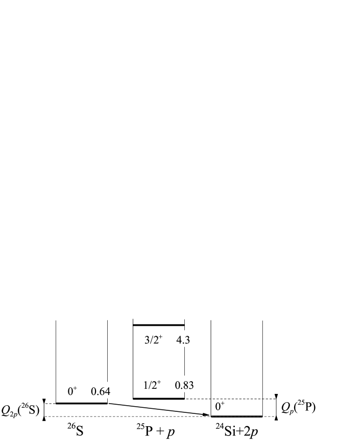
Figure 1: Energy levels and decay scheme for a possible true $2p$ decay of ²⁶S. The threshold energies are taken from systematics [17].

The ²⁶S nucleus has never been studied theoretically in details. It has been briefly mentioned in papers [18, 19] (phenomenology) as a possible $2p$ emitter. RMF calculations were performed in [20, 21, 22, 23]. The results of these studies for ²⁶S are quite controversial (information relevant to ²⁶S and its subsystems is summarized in Table 1). The predicted $2p$-decay energies are scattered in a broad range between 0 and 2 MeV, and the radial characteristics vary considerably as well. The overall situation is such that the existing theoretical information is not very helpful for planning experimental search for ²⁶S. It is not even clear if ²⁶S is a true two-proton emitter [$Q_{p}(^{25}$P$)>Q_{2p}(^{26}$S$)$] or sequential one-proton emission is possible for this nucleus [$S_{p}(^{26}$S$)<0$]. The lifetime vs decay energy systematics are drastically different in these cases. There are theoretical works supporting both possibilities and absolutely no experimental data.

We would like to provide some support for the true $2p$ character of the ²⁶S decay using the recent experimental data on ¹⁹Mg [13]. A negative value of $S_{p}=-0.42$ MeV was inferred for ²⁶S in Ref. [18] basing on the $\Delta_{pn}$ vs $S_{p}$ systematics. Here $\Delta_{pn}(Z)=S_{n}(^{A}_{Z}N)-S_{p}(^{A}_{N}Z)$ is the difference of the nucleon separation energies in isobaric mirror partners. It was assumed in Ref. [18] that the $\Delta_{pn}$ behaviour should be smooth and thus a value of $\Delta_{pn}\sim 6$ MeV was estimated for ²⁶S (in contrast with $\Delta_{pn}=5.39$ predicted by [17]). This systematics is shown in Fig. 2 but together with the same ones for the neon and magnesium chains. One can easily see that for the known true $2p$ emitters ¹⁶Ne and ¹⁹Mg, also belonging to the $s$-$d$ shell, there is a break in the smooth trend of $\Delta_{pn}$. Such a break could be connected, for example, to structural peculiarities of the three-cluster systems in proximity to the proton dripline [24]. The $\Delta_{pn}$ value is shifted downwards by 0.35-0.5 MeV for the known neighbouring systems when we pass the proton dripline. This observation is in a good agreement with the prediction of Ref. [17] for ²⁶S supporting the idea about the true $2p$ character of the ²⁶S decay.

The discussed situation motivated us to make first a dedicated theoretical study of ²⁶S focusing on the possibility of true two-proton emission and then to perform an experimental search for ²⁶S if the theoretical results look promising.

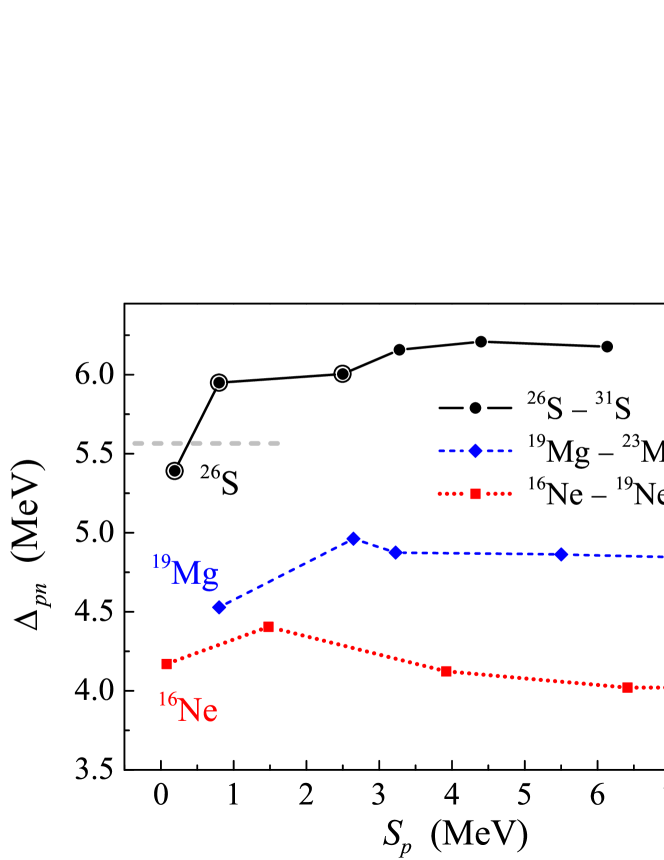
Figure 2: Systematics $\Delta_{pn}$ vs $S_{p}$. For the neon and magnesium chains the values are experimental; for the sulphur chain they are partly taken from systematics Ref. [17] (dots with circles around). Below the gray dashed horizontal line the $S_{p}$ value for ²⁶S is positive (it is a true two-proton emitter) and above it is negative (the sequential one-proton decay becomes possible).

2 The many-body structure aspect of the $2p$ decay

Our approach to the $2p$ radioactivity problem [2] is based on the approximate boundary conditions for the Coulomb three-body problem formulated in Ref. [3]. The three-body wave function (WF) $\Psi_{3}^{(+)}(\rho,\Omega_{5})$ with pure outgoing boundary conditions and complex energy $E=Q_{2p}-i\Gamma/2$ is constructed for an arbitrary small value of $\Gamma$ using the hyperspherical harmonic method. In this method the WF depends on the collective variable hyperradius $\rho$ and on the 5-dimensional hyperangle $\Omega_{5}$. After that the actual $\Gamma$ is found using the “natural” definition

$$\Gamma=\frac{j}{N}=\frac{\text{Im}\int\!d\Omega_{5}\left.\Psi^{(+)\dagger}_{3}\rho^{5/2}(d/d\rho)\rho^{5/2}\Psi^{(+)}_{3}\right|_{\rho_{\max}}}{||\Psi_{3}^{(+)}||^{2}}\,.$$ (1)

The differentials of the flux $j$ defined on the hypersphere with large hyperradius $\rho_{\max}\sim 10^{3}$ fm and the classical trajectory extrapolation to $\rho_{\text{ext}}\sim 10^{5}$ fm are used to define the momentum distributions (see Refs. [4, 5, 7] for technical details).

The three-cluster approach to the $2p$ decays is well justified for the closed-shell systems or systems with a closed-shell core. However, most of the two-proton emitters, including ²⁶S, do not belong to this class, and important effects of the many-body structure can be expected for them. The major components of the three-body cluster WFs with $J^{\pi}=0^{+}$ can be written in a schematic spectroscopic notation as

$$\Psi_{3}^{(+)}=\sum\nolimits_{i}X_{i}[l_{i}^{2}]_{0}\quad;\qquad\sum\nolimits_{i}|X_{i}|^{2}\lesssim 1\,.$$ (2)

The schematic notation $[l_{i}^{n}]_{J}$ denotes the Slater determinant of $n$ nucleons occupying $l_{i}$ orbital projected on the total spin $J$ and normalized: the three-body WF can be considered as normalized in the internal region

$$||\Psi_{3}^{(+)}||^{2}=\int d\Omega_{5}\int_{0}^{\rho_{\max}}d\rho\,\rho^{5}|\Psi_{3}^{(+)}|^{2}\equiv 1$$ (3)

without loss of generality. In papers [4, 5] the results of the $2p$ width calculations were provided as functions of weights of the main cluster configurations $w(l^{2}_{i})=X_{i}^{2}$. Therefore we can write

$$\Gamma(X^{2}_{i})=j(X^{2}_{i})\,.$$ (4)

The values which can be put in correspondence with the components of the three-body WF (2), to take into account the many-body structure, are overlaps of the many-body WFs of the precursor-daughter pair multiplied by a combinatorial term

$$\Psi_{A,A-2}=\left(\frac{A!}{2!(A-2)!}\right)^{1/2}\langle\Psi_{A}|\Psi_{A-2}\rangle=\sum_{i}\tilde{X}_{i}[l_{i}^{2}]_{0}\,.$$ (5)

The overlaps of Eq. (5) are in general case not normalized to unity:

$$N_{2p}=\sum\nolimits_{i}|\tilde{X}_{i}|^{2}\neq 1\,.$$ (6)

If we normalize them to unity, $\Psi_{A,A-2}\rightarrow\Psi_{A,A-2}N_{2p}^{-1/2}$, then the initial many-body WF becomes not normalized to unity $||\Psi_{A}||=N_{2p}^{-1}$. According to Eq. (1) the width should be then renormalized as

$$\tilde{\Gamma}=N_{2p}\,\Gamma(\tilde{X}^{2}_{i}/N_{2p})\,.$$ (7)

The renormalized width contains a product with structural factor ($N_{2p}$) which can be easily interpreted as a kind of a spectroscopic factor in analogy with the two-body decays. However, contrary to the two-body case, the dependence of the width on the structure includes the dependence on the amplitudes $X_{i}$. They should be adjusted as $X_{i}\rightarrow\tilde{X}_{i}/\sqrt{N_{2p}}$. That makes the above renormalization a complicated nonlinear procedure. We will see below that the many-body effects lead to a significant renormalization of the width beyond the Hartree approximation.

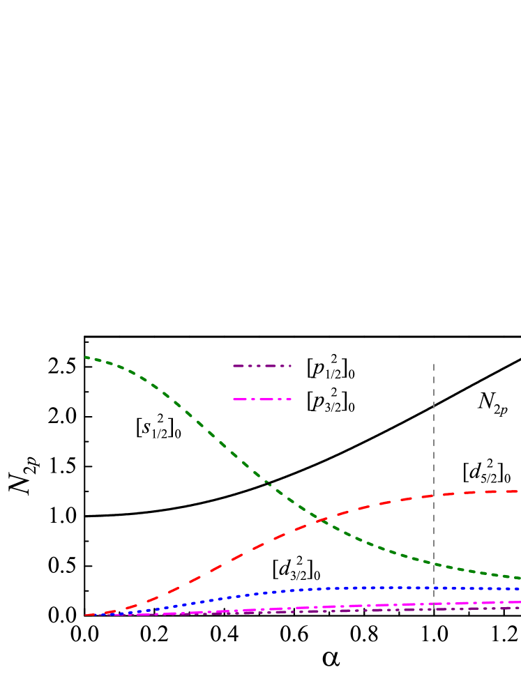
Figure 3: (Colour online) Weights of the major components of the overlaps Eq. (5) (left axis) and the total overlap normalization as a function of the parameter $\alpha$ (right axis). This parameter scales the pairing gap $\Delta\rightarrow\alpha\Delta$.

To calculate the amplitudes $\tilde{X}_{i}$ in a many-body approach we can use a formalism analogous to the same intrinsic structure model as for direct two-nucleon transfer reactions [for instance, pick-up processes ($p,t$), ($n$,³He) etc]. In the present work we consider the following situation: (i) both the parent nucleus $Z$ and the daughter nucleus $Z-2$ are essentially many-body systems, (ii) both nuclei are spherical in their ground states, (iii) the emitted proton pair transfers zero total angular momentum, (iv) both nuclei remain in their ground states.

The structure part of the two-nucleon transfer cross section is determined by the spectroscopic amplitude $B$ which is defined in the second quantization formalism as [25, 26]:

$$B_{(K_{i}K_{f},kk^{\prime})}^{J}=\sum\limits_{MM_{i}}C_{J_{i}M_{i}JM}^{J_{f}M_{f}}\langle\Psi_{K_{f}}|\mathcal{O}_{(kk^{\prime})}^{JM}|\Psi_{K_{i}}\rangle,$$ (8)

where $K_{i}=\{(K_{i}),M_{i}\}$ and $K_{f}=\{(K_{f}),M_{f}\}$ denote quantum number sets of the initial and final nuclei with $\bigl{(}K_{i};K_{f}\bigr{)}$ and without $\bigl{(}(K_{i});(K_{f})\bigr{)}$ angular momentum projections $M_{i}$, $M_{f}$. Index $k$ denotes the full set of the single-particle quantum numbers $k=\{(k),m_{k}\}$ in a spherical nucleus. $\mathcal{O}$ is the two-nucleon transfer operator:

$$\mathcal{O}_{(kk^{\prime})}^{JM}=\frac{1}{1+\delta_{(kk^{\prime})}}\sum\limits_{m_{k}m_{k^{\prime}}}C_{j_{k}m_{k}j_{k^{\prime}}m_{k^{\prime}}}^{JM}a_{k}a_{k^{\prime}}\,,$$ (9)

where $a_{k}$ is the nucleon annihilation operator in the mean field basis.

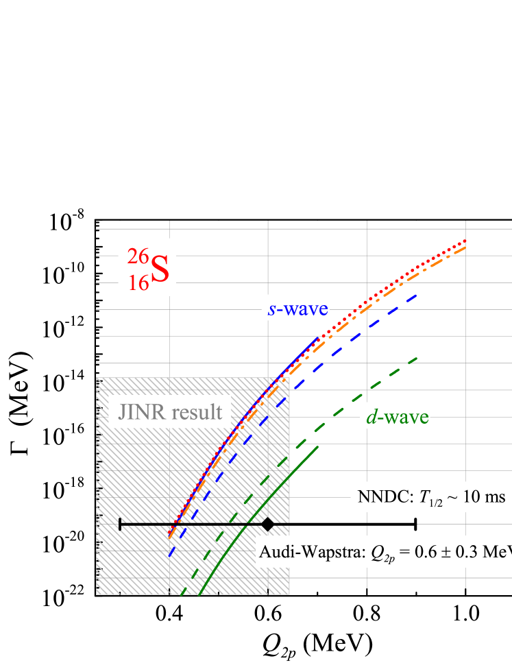
Figure 4: (Colour online) Width of the ²⁶S g.s. as a function of the $2p$ decay energy. Solid and dashed curves correspond to the quasiclassical simultaneous emission model and to the three-body “$l^{2}$” model, respectively. The RMF-assisted three-body model, based on the relativistic Hartree (RH) and on the complete RH+BCS results are shown by the dotted and by the dash-dotted curves, respectively. The lower hatched area shows the energy and the half-life ranges excluded by the current experiment.

For the ground states of both parent and daughter nuclei we apply the Bardeen-Cooper-Schrieffer (BCS) approximation. In this model the ground state WF of an even-even spherical nucleus reads:

$$|\Psi_{K}\rangle=|K;\text{BCS}\rangle=\prod_{k>\ 0}\bigl{(}u_{(k)}+v_{(k)}a^{\dagger}_{k}a^{\dagger}_{\bar{k}}\bigr{)}|-\rangle\,,$$ (10)

where $|-\rangle$ is the bare vacuum. In the case of time-reversal symmetry for each state $k>0$, there exists a corresponding time-reversed state ${\bar{k}}<0$ so that all the states $\{k,{\bar{k}}\}$ together form the whole single-particle space. The spectroscopic amplitude defined in Eq. (8) takes the form:

$$\tilde{X}_{(k)}=B_{(K_{i}K_{f},kk)}^{0}=\sqrt{\Bigl{(}j_{k}+\frac{1}{2}\Bigr{)}}\,u_{(k)}^{(Z-2)}v_{(k)}^{(Z)}\,.$$ (11)

3 Structure of ²⁶S in RMF

In the present work we employ a RMF model based on the covariant NL3 density functional [27]. Numerous calculations with NL3 parametrization have demonstrated excellent agreement with data in nuclear masses, deformation properties [27] and properties of giant resonances and nuclear low-lying response [28]. In RMF model the single-nucleon wave function is a Dirac spinor characterized by the set $k=\{(k),m_{k}\}$ and $(k)=\{n_{k},j_{k},\pi_{k},{\tau}_{k}\}$ with the radial quantum number $n_{k}$, angular momentum quantum numbers $j_{k},m_{k}$, parity $\pi_{k}$ and isospin ${\tau}_{k}$, see Ref. [29] for details. For the pairing interaction we use a monopole-monopole ansatz. The BCS gap equation is solved self-consistently with the RMF set of equations as described in Ref. [28]. The strength of the pairing interaction was adjusted in such a way that the binding energy of ²⁴Si and the phenomenological proton pairing gap in ²⁶S are well reproduced.

The results of the RMF calculations important for $2p$ decay are summarized in Table 1 and Fig. 3. The figure demonstrates evolution of the ²⁶S structure with the scaling of the pairing gap. In the relativistic Hartree (RH) case ($\alpha=0$) only the nearest to the Fermi surface $s_{1/2}$ single-particle configuration contributes to $2p$ decay and the renormalization of the width is trivial ($N_{2p}=1$). For realistic values of the pairing gap ($\alpha\sim 1$) the valence configuration structure for ²⁶S is characterized by the strong configuration mixing with a dominance of the $[d_{j}^{2}]_{0}$ configurations.

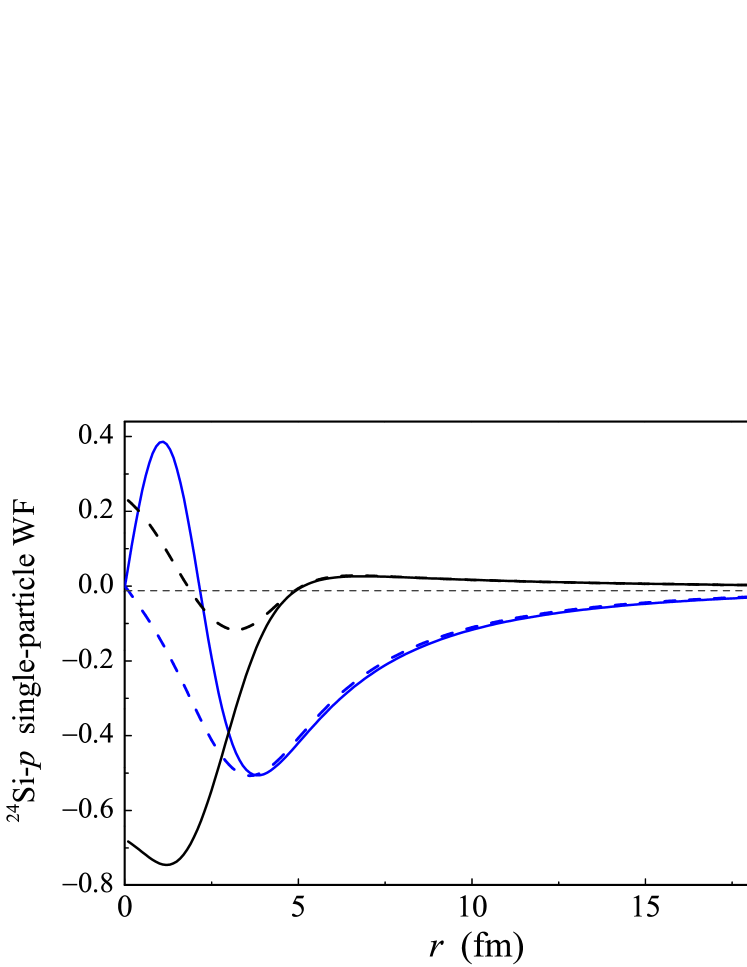
Figure 5: (Colour online) Black solid line shows the scaled mean field potential reproducing the proton separation energy (right axis). Black dashed line shows the potential with a repulsive core excluding the $s$-wave forbidden state. Single-particle $s$-wave WFs (found on resonance) are shown for these potentials by the blue curves of the corresponding style (left axis).

4 Three-body $2p$ decay calculations

The simple half-life estimates for ²⁶S are provided in Fig. 4 in terms of the models based on systematic values of parameters which we have broadly used before. The quasiclassical simultaneous emission model [5] neglecting the interaction between the protons provides a broad “belt” of half-life values between the boundaries connected to emission from the $[s^{2}]_{0}$ (upper width limit) and $[d^{2}]_{0}$ (lower width limit) configurations. The three-body “$l^{2}$” model [4] predicts somewhat narrower belt of possible half-lives (however, it is still as broad as two orders of magnitude).

The RMF results are utilized to modify the three-body calculations in two ways. (i) The RMF potentials are used to create the core-$p$ interactions for the three-body model. (ii) The three-body internal structure of the ²⁶S is adjusted to be reasonably close to the structure predicted by RMF with a help of phenomenological short range potentials in $\rho$ variable acting on the selected hyperspherical components of the WFs $\Psi_{3}^{(+)}$.

The RMF potential is fitted by the two Woods-Saxon components with $V_{0}=\{26,-90\}$ MeV, $r_{0}=\{0.8,2.87\}$, $a=\{0.55,0.75\}$ fm ($V_{ls}=-14.3$ MeV, $r_{0}=2.87$, $a=0.75$ fm), see Fig. 5. The depth of this potential is scaled to get the RMF positions of the $p$- and $d$-waves in the nonrelativistic Schrödinger equation. For the $s$-waves the modified potential is used $V_{0}=\{32.7,-19\}$ MeV, $r_{0}=\{1.5,4.15\}$, $a=\{0.8,0.63\}$ fm, which contains the core and thus excludes the Pauli forbidden deep $s$-state. The $2p$ width is very sensitive to the WF behaviour on the nuclear surface. It can be seen in Fig. 5 that the surface behaviour of the WF in the modified potential is practically identical to that of the initial potential. The Coulomb potential in the core-$p$ channel is derived using the charge distribution of ²⁴Si obtained in the RMF calculations. The simple single Gaussian $s$-wave potential $V(r)=-31\exp[-(r/1.8)^{2}]$ is used in the $p$-$p$ channel.

Thus, the difference of the RMF-assisted three-body results shown in Fig. 4 compared to results of our ordinary “$l^{2}$” calculations has the following three sources. (i) The core-$p$ interactions are not taken from systematics [$r_{0}=1.2(A_{c}+1)^{1/3}$ fm] but are constructed using the RMF results. The width is somewhat increased by this choice of the core-$p$ interactions. (ii) The three-body structure of ²⁶S is adjusted to the relative weights of the two-proton overlap functions obtained in the RMF calculations. This leads to the width reduction compared to the pure three-body calculations. (iii) The $2p$ width value should be renormalized according to the value $N_{2p}$ of the two-proton overlap functions obtained in the RMF calculations. For the predicted structure of ²⁶S this leads to the increase of the width by a factor of two. The latter two trends partly compensate each other. Thus, at least for the case of ²⁶S decay, taking the many-body structure of the $2p$ emitter into account leads to the results which are less sensitive to model assumptions. The predictive ability of the model is therefore expected to be higher even for quite a simplistic method of the structure treatment used in this work.

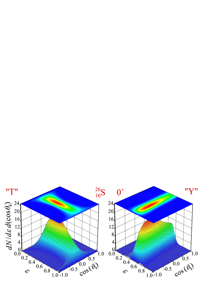
Figure 6: (Colour online) Kinematically complete correlation patterns for the $2p$ decay of ²⁶S g.s. in the “T” Jacobi system ($\varepsilon$ scales the relative energy between two protons) and in the “Y” Jacobi system ($\varepsilon$ scales the energy between the daughter nucleus ²⁴Si and one of the protons). Angles $\theta_{k}$ are defined in Eq. (12).

This model has important features which we would like to emphasize: (i) the internal structure of the three-body WF corresponds well to the structure of the overlaps predicted in RMF (ii) penetration through the Coulomb barrier is entirely defined by the $p$-$p$ interaction and the single-particle structure of the core+$p$ subsystems.

Predicted complete momentum correlations for the $2p$ decay of ²⁶S are shown in Fig. 6 in terms of the energy distribution parameter $\varepsilon$ and angle $\theta_{k}$ between the Jacobi momenta $\mathbf{k}_{x}$, $\mathbf{k}_{y}$:

$$\varepsilon=E_{x}/E_{T}\quad,\quad\cos(\theta_{k})=(\mathbf{k}_{x}\cdot\mathbf{k}_{y})/(k_{x}\,k_{y})\,,$$

$$E_{T}=E_{x}+E_{y}=k^{2}_{x}/2M_{x}+k^{2}_{y}/2M_{y}\,,$$

$${\bf k}_{x}=\frac{A_{2}{\bf k}_{1}-A_{1}{\bf k}_{2}}{A_{1}+A_{2}}\,,\,\;{\bf k}_{y}=\frac{A_{3}({\bf k}_{1}+{\bf k}_{2})-(A_{1}+A_{2}){\bf k}_{3}}{A_{1}+A_{2}+A_{3}}\,.\;$$ (12)

where $M_{x}$ and $M_{y}$ are the reduced masses of the $X$ and $Y$ subsystems (see, e.g. [6] for details). The correlation patterns demonstrate the regions of strong suppression, connected with the repulsive core-proton Coulomb interaction [$\varepsilon\sim 0.5$, $\cos(\theta_{k})\sim\pm 1$ in the “T” system]. Another feature is a broad peak [$\cos(\theta_{k})\sim 0$ in the “T” system] connected with the large weight of the $s$-wave configuration in ²⁶S. Similar correlation patterns have been obtained for other $s/d$-shell $2p$ emitters [4] and were later found to be in agreement with the experimental data in Ref.  [31].

Results of the theoretical studies indicate that the considerations for further experimental searches for ²⁶S are especially complicated. If we take the standard energy prescription made by Audi and Wapstra [17] then we have a $50\%$ “probability” that ²⁶S can be studied in an implantation experiment (half-life exceeding $\sim 100$ ns – the typical flight-time for the fragment separation). Otherwise the decay-in-flight technique [13] can be used for the ²⁶S study down to half-life times as short as some picoseconds. The $Q_{2p}$ predictions made by different theoretical models point at higher energies $Q_{2p}\gtrsim 0.8$ MeV but do not seem to provide a solid basis for the choice of experimental technique. We decided to make the first attempt to study ²⁶S in the implantation experiment.

5 Experiment

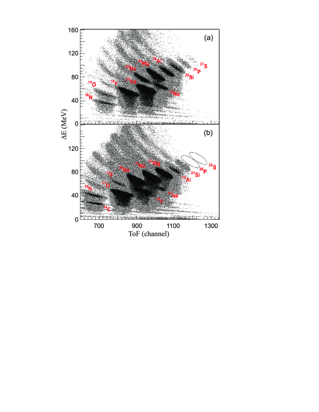
Figure 7: (Colour online) $\Delta E$-ToF identification plots for the cases of separator tuning on ²⁷S (a) and ²⁶S (b).

The experiment was performed at the ACCULINNA fragment separator [30] (JINR, Dubna, Russia). A 50.3 A MeV beam of ³²S¹¹⁺ ions delivered by the U400M cyclotron with intensity up to 30 pnA bombarded a 92.4-mg/cm² beryllium production target installed in the separator object plane. A 92.4-mg/cm² beryllium wedge was installed in the intermediate focal plane of the separator. Combined with a slit restricting the momentum acceptance to about $2.0\%$, this rather thick wedge reduced in number the set of ³²S fragmentation products arriving at the achromatic focal plane when the separator was tuned for a desired product with its specific charge $Z$ and mass $A$. Mostly, the nuclei arriving in the beam cocktail at the final focal plane of the separator were severely depleted in intensity. This provided favourable conditions to detect ²⁶S anticipated to be a very rare product of the ³²S fragmentation. It turned out that only a few fragmentation products with different $Z$ and $A$ occurred to be close in transmission probability to the searched nucleus. This appeared to be useful as such “satellites” were used for tuning the separator when rare fragments, such as ²⁶S, were searched for.

To ensure unequivocal identification for the nuclei passing through the separator we used both the time-of-flight-$\Delta E$ (ToF-$\Delta E$) and $\Delta E$-$E$ techniques. The ToF array, having about 0.6 ns time resolution, was placed on a 8.5-meter flight base between the achromatic and final focal planes of the separator. The ToF detectors were two 125-$\mu$m thick BC-418 plastics inclined at $45^{\circ}$ to the separator axis and each plastic viewed by its pair of XP2020 photomultipliers. The telescope composed of one 68-$\mu$m and one 1000-$\mu$m, $6\times 6$ cm² silicon strip detectors ($8\times 8$ strips) was installed in the final focal plane. Besides the $\Delta E$-$E$ identification the hit positions of the nuclei were measured by this telescope. Also, the signals from the telescope $\Delta E$ detectors were used for the ToF-$\Delta E$ identification. In all the runs the load of the strip detectors did not exceed 500 pps. Taking into account the granularity of these detectors such counting rate makes pileups negligible.

Four runs were performed in which the separator was sequentially tuned to give the optimum transmission for ²⁹S, ²⁸S, ²⁷S and ²⁶S. The measurements took 870, 1200, 4500 and $1.1\times 10^{5}$ seconds, respectively. For the two latter cases the $\Delta E$-ToF plots are presented in Fig. 7. No events of ²⁶S, as well as ²⁵P, were found in the measurements. To extract the upper lifetime limits for these nuclei, the isotope yields of some known nuclei from sulphur to neon were systematized depending on their reaction $Q$ values, see Fig. 8. In this figure the results of runs tuned for the sulphur isotopes are shown. In addition to the three sulphur isotopes (²⁷S, ²⁸S and ²⁹S) the yields of nuclei representing the “satellites” in the four separator tunes are presented in Fig. 8 (a). These satellites are the nuclei having parameter $A^{5/2}/Z^{3/2}$ close to that of the tuned sulphur isotopes (variation from $-4\%$ to $+3\%$ was allowed). This parameter defines the selectivity of the energy loss achromat. For the nuclei selected in such a way the yield dependence on the reaction $Q$ values should have exponential character reasonably close to the exponential dependence of the production cross sections. Both the yield and the cross section dependence on $Q_{\text{reaction}}$ is given in Fig. 8 (b) for a subset of these nuclei having high transmission rates through the fragment separator, namely above $0.25\%$. Naturally, these appear to be sulphur, phosphorus, and silicon isotopes. The cross sections were defined using the transmission rates calculated with the use of relations from Ref. [32].

The main contribution to the experimental errors stems from the systematic uncertainties of both the flux of the ³²S primary beam and the transmission through the separator. It was estimated to be about $25\%$. The extrapolation of the obtained systematics shows that in the presented experiment one could expect the observation of $16^{+6}_{-4}$ and $360^{+85}_{-70}$ events of ²⁶S and ²⁵P, respectively. The total length of the ACCULINNA separator from the production target to the final focus position is 21.3 m. The full times of flight for these nuclei from the production target to the detector system were $314$ ns and $322$ ns (accounting for energy losses in the wedge and ToF-plastics). Using the Poisson distribution the half-life limit for ²⁶S can be found as $T_{1/2}(^{26}$S$)<79$ ns with $63\%$ confidence level and $T_{1/2}(^{26}$S$)<157$ ns with $98\%$ confidence level. In these estimations one and four events respectively were assumed instead of observed zero events. The 79 ns half-life limit is in qualitative agreement with nonobservation of ²⁶S as an expected accompanying nucleus in the recent experiment with a ²⁴Si secondary beam at MSU [33].

The corresponding half-life limits for ²⁵P are found as $T_{1/2}(^{25}$P$)<38$ ns and $T_{1/2}(^{25}$P$)<50$ ns. The $38$ ns half-life limit is compatible with the limit of $30$ ns provided in Refs. [16, 17, 34] (this value seems to be based on an unpublished work). It can be easily estimated that such a limit provides quite a relaxed limit for the proton decay energy in ²⁵P: $Q_{p}(^{25}$P$)\gtrsim 110$ keV (according to an R-matrix estimate with systematic parameters). This is not a restrictive result to define the character of the ²⁶S decay (true or sequential $2p$ decay, see Table 1 and relevant discussion in the introduction). However, it helps to provide a two-proton decay energy limit for ²⁶S.

Using the dependence shown in Fig. 4 we find that a half-life limit of $79$ ns provides a $2p$-decay energy limit $Q_{2p}(^{26}$S$)>640$ keV assuming the true two-proton decay. If the one-proton decay were possible for this nucleus (which we find to be unlikely situation, but cannot exclude completely) one would get a limit for one-proton decay energy $Q_{p}(^{26}$S$)>120$ keV (R-matrix estimate). Combining it with $Q_{p}(^{25}$P) limit we obtain a limit $Q_{2p}(^{26}$S$)>230$ keV. The previously reported half-life value of 10 ms [16] belongs to the timescale where the decay can be attributed to the weak transitions as well (nucleus with such a half-life could appear to be even nuclear stable). The half-life times in the nanosecond range and shorter would undoubtfully identify the ²⁶S nucleus as a $2p$ emitter.

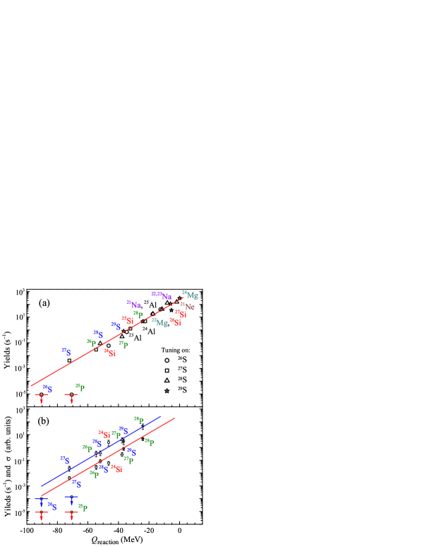
Figure 8: (Colour online) Panel (a) shows the yields of different nuclei as a function of the reaction $Q$ value. In this panel the symbol size is comparable with the error bar values. Panel (b) shows the yields (lower group of symbols, red line) and production cross sections (upper group of symbols, blue line) for the isotopes with highest transmission rate through the fragment separator.

6 Conclusions

We have studied both theoretically and experimentally properties of the proton dripline nucleus ²⁶S. Structures of ²⁶S and its subsystems (²⁴Si, ²⁵P) were obtained in the RMF approach. The $2p$ decay properties of ²⁶S were obtained in a three-body model tuned by the RMF results. It is demonstrated that in this joint approach the results appear to be noticeably different than the results of the three-body “$l^{2}$” model based on a systematics input. The uncertainties of the $2p$ width connected with structure of $2p$ emitters are significantly reduced in this approach.

Production of ²⁶S in the fragmentation reaction was studied experimentally. We have found that either the production of ²⁶S is anomalously small (more than one order of magnitude than expected according to systematics) or the lifetime is too short. The systematical value of the production cross section enables us to estimate the upper half-life limit of ²⁶S as 79 ns. Theoretical lifetime dependence on the $2p$-decay energy allows one to infer the lower limit of 640 keV for the $Q_{2p}$ of ²⁶S. This value is in principle consistent with the theoretically predicted range of mass excess for ²⁶S but it narrows significantly its uncertainty. In the case that ²⁶S has an open one proton decay branch (sequential two-proton decay) a less restrictive limit $Q_{2p}>230$ keV is obtained.

Our results are in contradiction with the existing information about ²⁶S as a possible $2p$ emitter with the half-life of about 10 ms [16]. Our results allow focusing the search for ²⁶S in the half-life range 10 ps – 100 ns where the decay-in-flight technique [13] is the adequate experimental method.

References

- [1] V.I. Goldansky, Nucl. Phys. 19 (1960) 482.
- [2] L.V. Grigorenko et al., Phys. Rev. Lett. 85 (2000) 22.
- [3] L.V. Grigorenko et al., Phys. Rev. C 64 (2001) 054002.
- [4] L.V. Grigorenko, M.V. Zhukov, Phys. Rev. C 68 (2003) 054005.
- [5] L.V. Grigorenko, M.V. Zhukov, Phys. Rev. C 76 (2007) 014008.
- [6] L.V. Grigorenko et al., Phys. Lett. B677 (2009) 30.
- [7] L.V. Grigorenko et al., Phys. Rev. C 82 (2010) 014615.
- [8] M. Pfützner et al., Eur. Phys. J. A 14 (2002) 279.
- [9] J. Giovinazzo et al., Phys. Rev. Lett. 89 (2002) 102501.
- [10] B. Blank et al., Phys. Rev. Lett. 94 (2005) 232501.
- [11] C. Dossat et al., Phys. Rev. C 72 (2005) 054315.
- [12] J. Giovinazzo et al., Phys. Rev. Lett. 99 (2007) 102501.
- [13] I. Mukha et al., Phys. Rev. Lett. 99 (2007) 182501.
- [14] K. Miernik et al., Phys. Rev. Lett. 99 (2007) 192501.
- [15] L.V. Grigorenko, I.G. Mukha, M.V. Zhukov, Nucl. Phys. A713 (2003) 372; erratum A740 (2004) 401.
- [16] NNDC BNL database, http://www.nncc.bnl.gov.
- [17] G. Audi et al., Nucl. Phys. A729 (2003) 3.
- [18] B.A. Brown, P.G. Hansen, Phys. Lett. B381 (1996) 391.
- [19] B.J. Cole, Phys. Rev. C 58 (1998) 2831.
- [20] S.K. Patra, R.K. Gupta, W. Greiner, Int. J. Mod. Phys. E6 (1997) 641.
- [21] G.A. Lalazissis, A.R. Farhan, M.M. Sharma, Nucl. Phys. A628 (1998) 221.
- [22] B.Q. Chen et al., J. Phys. G: Nucl. Part. Phys. 24 (1998) 97.
- [23] Z. Wang and Z. Ren, Nucl. Phys. A794 (2007) 47.
- [24] L.V. Grigorenko et al., Phys. Rev. Lett. 88 (2002) 042502.
- [25] S. Yoshida, Nucl. Phys. 33 (1962) 685.
- [26] R.A. Broglia, C. Riedel, Nucl. Phys. A92 (1967) 145.
- [27] G.A. Lalazissis, J. König, P. Ring, Phys. Rev. C 55 (1997) 540.
- [28] E. Litvinova, P. Ring, V. Tselyaev, Phys. Rev. C 78 (2008) 014312.
- [29] Y.K. Gambhir, P. Ring, A. Thimet, Ann. Phys. (N.Y.) 198 (1990) 132.
- [30] A.M. Rodin, et al., Nucl. Instr. Meth. A391 (1997) 228.
- [31] I. Mukha et al., Phys. Rev. C 77 (2008) 061303.
- [32] J.A. Winger, B.M. Sherrill, D.J. Morrissey et al., Nucl. Instr. Meth. B70 (1992) 380.
- [33] A. Gade et al., Phys. Rev. C 77 (2008) 044306.
- [34] R.B. Firestone, Nucl. Data Sheets 110 (2009) 1691.