Measuring the Clump Mass Function in the Age of SCUBA2, Herschel, and ALMA

Abstract

We use simulated images of star-forming regions to explore the effects of various image acquisition techniques on the derived clump mass function. In particular, we focus on the effects of finite image angular resolution, the presence of noise, and spatial filtering. We find that, even when the image has been so heavily degraded with added noise and lowered angular resolution that the clumps it contains clearly no longer correspond to pre-stellar cores, still the clump mass function is typically consistent with the stellar initial mass function within their mutual uncertainties. We explain this result by suggesting that noise, source blending, and spatial filtering all randomly perturb the clump masses, biasing the mass function toward a lognormal form whose high-mass end mimics a Salpeter power law. We argue that this is a consequence of the central limit theorem and that it strongly limits our ability to accurately measure the true mass function of the clumps. We support this conclusion by showing that the characteristic mass scale of the clump mass function, represented by the “break mass”, scales as a simple function of the angular resolution of the image from which the clump mass function is derived. This strongly constrains our ability to use the clump mass function to derive a star formation efficiency. We discuss the potential and limitations of the current and next generation of instruments for measuring the clump mass function.

1. Introduction

The mass function of molecular cloud clumps is increasingly being used as a tool to test theories of star formation. By comparing the mass function of pre-stellar molecular cloud cores to the initial mass function (IMF) of stars, one hopes to constrain things like the efficiency and timescales of star formation. Similarly, one can test different theories of star formation by comparing the clump mass functions they predict to the observations. The potential for using the clump mass function as a diagnostic of massive star formation is particularly attractive. There is no clear one-to-one relationship between individual massive stars and individual pre-stellar molecular cloud cores. Massive stars may form by competitive accretion, by monolithic collapse of a molecular cloud core, or some combination. Presumably these two theories could be distinguished on the basis of the clump mass functions they predict.

In recent years, measurements of the shape of the clump mass function in nearby low-mass star-forming regions have demonstrated good agreement with the shape of the stellar initial mass function (Testi & Sargent, 1998; Motte, André, & Neri, 1998; Motte et al., 2001; Johnstone et al., 2000, 2001; Tothill et al., 2002). The slopes of the high-mass ends of the stellar IMF and the clump mass function agree within their uncertainties. The two mass functions peak at different masses, but this is taken to be indicative of the star formation efficiency. These quantitative resemblances between the stellar IMF and the clump mass function have been interpreted as evidence that the clumps we observe are the direct precursors of individual low-mass stars (or low-order multiples).

Our ability to use the clump mass function as a test of theories of star formation hinges crucially on our ability to measure it accurately and interpret it confidently. In this paper, we will argue that the observations to date have not provided definitive measurements of either the shape or the characteristic mass scales of the clump mass function. We will also argue that this situation may be about to change, thanks to upcoming observations to be made with instruments such as the Submillimetre Common-User Bolometer Array 2 (SCUBA2, Robson & Holland 2007) on the James Clerk Maxwell Telescope (JCMT) as well as the Spectral and Photographic Imaging Receiver (SPIRE, Griffin et al. 2009) and the Photodetector Array Camera and Spectrometer (PACS, Poglitsch & Altieri 2009) on the Herschel Space Observatory.

Reid & Wilson (2006b) began this investigation by showing that the interpretation of observational clump mass functions is biased by the effects of small-number statistics and certain fitting techniques. Reid & Wilson (2006b) hypothesized that the observed shape of the clump mass function may be determined as much by our observational and analytical techniques as by the physics of star-forming clouds. They showed that a lognormal shape provides the best fit, with the fewest parameters, to the observed clump mass functions, but they could not draw hard conclusions about the origin of this lognormal shape. In this paper, we will extend this analysis, arguing that our observational techniques play a role in determining the functional form of the clump mass function, biasing it toward a lognormal shape.

2. Analysis

2.1. Problems in the Interpretation of Clump Mass Functions

From an observational perspective, there is a very important distinction between stars and clumps. Stars appear as points whose luminosities can be measured accurately, save for relatively small, quantifiable uncertainties due to binarity and crowding. Clumps, on the other hand, are extended objects viewed against a background of emission from their parent molecular clouds and from Galactic cirrus. The flux one measures from a clump can depend strongly on, among other things, the noise level in the image, the angular resolution of the image, projection effects, image processing techniques that might be used during or after data acquisition, and the choice of clump-finding algorithm. Each of these effects varies in magnitude with the mass and internal structure of the clump so the whole mass function is not evenly affected.

To interpret a clump mass function, it is necessary to know how it was measured. The most common method is to measure the clump mass function from images of thermal dust emission at millimeter and submillimeter wavelengths. Another common method uses molecular line maps analysed using routines such as GAUSSCLUMPS (e.g. Kramer et al. 1998, Stutzki & Guesten 1990) or, more recently, dendrogram methods (Rosolowsky et al., 2008). A further method extracts the clumps from dust extinction maps (Alves, Lombardi, & Lada, 2007). We concentrate on the dust continuum observations here, both because of their popularity in the past and because they will be produced in quantity by instruments such as Herschel, SCUBA2, and ALMA.

Maps of the dust continuum emission in star-forming regions show a combination of discrete clumps and smooth, often filamentary structures. These structures are sectioned into clumps either by eye (Testi & Sargent, 1998; Tothill et al., 2002) or using one of a variety of algorithms, such as clfind2d (Williams, de Geus, & Blitz, 1994). Recently, clfind2d has been criticized for its inability to, among other things, produce accurate mass functions in regions where the emission is crowded or has a lot of structure on multiple spatial scales (Pineda, Rosolowsky, & Goodman, 2009; Kauffmann et al., 2010; Curtis & Richer, 2010). These are reasonable criticisms of clfind2d but, as we will argue throughout the rest of this section, our concerns about the interpretation of the clump mass function apply to many different clump-finding algorithms.

Clump mass functions are subject to several uncertainties which cannot be addressed easily with existing observations. Probably the most significant among these is the conversion of flux to mass. This conversion depends on several parameters, including the emissivity, temperature, and opacity of the dust, which are not well characterized and probably vary both from clump to clump and within clumps. Typically, estimated values are assumed to hold for all clumps in the sample. However, it will be important to remember that the assumption of standardized values for the dust emissivity, temperature, and opacity and their application to the entire volume of each clump constitutes an essentially random perturbation to the mass of each clump. These “random” errors may be systematic in the sense that they bias all of the clump masses in the same direction–either too high or too low–but they will affect each clump’s mass by a different, unknown amount. The cumulative effect on the clump mass function of many such random errors may be significant.

The choice of clump-finding algorithm constitutes an additional uncertainty which is difficult to control. Any given algorithm may assign too much or too little of the background emission in the image to a given clump. Given that clump extraction algorithms typically do not pair submillimeter continuum maps with velocity information, many of these algorithms will identify gravitationally unbound clumps. Some attempts to exclude gravitationally unbound clumps is usually made, but these attempts depend on some knowledge of the internal structures of the clumps, which is also lacking.

Uncertainties due to the inclusion of clumps which have already formed one or more stars (i.e. those which are not “pre-protostellar”) can be mitigated when deep mid- and far-infrared data are available, but this has not historically been the case.

Superposition of clumps and filaments along the line of sight represents a final significant source of uncontrolled uncertainty. Superposition will tend to increase the measured masses of clumps but, again, by random, unknown amounts.

Little can be said so far about the cumulative quantitative effects of these uncertainties. Upcoming multi-wavelength observations with Herschel and SCUBA2 will help address uncertainties due to spatial variations in dust properties and afford a better understanding of the structures of clumps in nearby star-forming regions. The next generation of clump finding algorithms promise to improve the accuracy with which clump structures can be determined and their masses calculated. Still, there will continue to exist significant unquantified uncertainties.

In this paper, we set aside all of the aforementioned concerns and instead seek to quantify the effects of our image acquisition techniques on the clump mass function. Image acquisition techniques vary substantially from one telescope to another, but they essentially all consist of combinations of a small set of elemental processes. Images can have more or less noise, coarser or finer angular resolution, and they can be spatially filtered in several ways (e.g. chopping and interferometry). Each of these has some effect on measurements of the clump mass function. In this paper, we seek to explore and quantify these effects.

2.2. The Reference Image

Our goal is to evaluate accurately the effects on the clump mass function of image noise, limited angular resolution, and spatial filtering. We thus begin with a simulated image which has no instrumental noise, higher intrinsic angular resolution than any we wish to simulate, and flux on a wider range of spatial scales than those we wish to simulate. We call this image our ‘reference image’.

Our reference image was derived from a snapshot of a star-forming region simulated using smoothed-particle hydrodynamics. The simulation began with a spherical cloud of turbulent, isothermal gas at 10 K which was allowed to collapse under the influence of its own gravity. This has been a standard approach in the last several years (e.g. Bate et al. 2003). The simulation was large, with a mass similar to that inferred for typical star forming clouds (5000 M_⊙ with 36M particles). The simulated cloud was marginally bound, having an rms Mach number of 13.42 and an initial radius of 4 pc. As our primary interest was pre-stellar cores, sink particles were not used. The resolution (gravitational and hydrodynamical) was limited to 50 AU, corresponding to a maximum number density of $\sim 4\times 10^{7}$ cm^-3 (mean molecular weight 2.33) and a minimum Jeans Mass of $\sim 0.04$ M_⊙(330 particles). The simulation was performed in parallel using the GASOLINE code (Wadsley et al., 2004) and is described in more detail in Petitclerc (2009). Our reference image was developed from a snapshot of the simulation taken 130,000 years after the cloud began collapsing. That is the epoch at which dense cores have appeared but before radiative effects become significant on the spatial scales of interest to us.

We are interested in simulating the results of observations which produce two-dimensional images of (presumed) optically thin emission. Thus, we made our image by projecting the simulation along a randomly chosen axis, neglecting optical depth effects. This reference image is shown in Figure 1. All subsequent images used in our analysis are modified versions of this one.

Figure 1.— Column density map made by projecting our simulated the star-forming region along its z axis. Darker areas indicate higher column densities.

2.3. The Reference Clump Mass Function

Instruments such as SCUBA2 and Herschel are producing images containing so many clumps and sitting on such complex backgrounds of Galactic cirrus and extragalactic point sources that manual clump identification is now time-prohibitive. Manual source extraction is also undesirable because it does not produce consistent, repeatable results and therefore introduces an unnecessary variable in the study of the clump mass function. A huge variety of source extraction tools are being developed to handle these new types and volumes of data. For the reasons discussed previously, we will use clfind2d for our analysis, but we have taken care to use it in a consistent, automatic way to eliminate the variable of manual “tuning” of the results. Our method consists of measuring the rms noise, $\sigma$, in emission-free parts of the image and then setting the threshold and contour intervals in clfind2d to 3$\sigma$ and 2$\sigma$ respectively.

Figure 2.— Differential (upper panel) and cumulative (lower panel) mass functions of the cores in the reference image, shown in Fig. 1. The error bars are too small to be represented clearly in the cumulative mass function. The DCMF has a constant 100 objects per bin. The dashed lines in the upper panel indicate a mass function with a Salpeter slope, $dN/dM\propto M^{-2.35}$.

We always produce two different representations of the clump mass function: the differential clump mass function (DCMF), $dN/dM$, and the cumulative clump mass function (CCMF), $N(>M)$. In producing the DCMF for a given image, we use a fixed number of clumps per bin (rather than fixed bin widths), following the prescription of Maíz-Apellániz & Úbeda (2005) for producing reliable histograms. The DCMF and CCMF for the clumps extracted from the reference image in this manner are shown in Figure 2. We note that the uncertainties in the flux-to-mass conversion, discussed in §2.1, affect the observations but not our simulations, which track mass directly.

The evidence so far suggests that the clump mass function, like the stellar initial mass function, follows a Salpeter-like power-law of the form $dN/dM\propto M^{-\alpha}$ with $\alpha\simeq 2.35$ above about $0.1$–$1$ M_⊙. For comparison, we have drawn such a power-law on the DCMF in Figure 2. As is evident, the DCMF of the simulated clumps in their ‘native’ form is well-fit by a Salpeter-like power-law. Hence, we conclude that our simulations replicate the observations well enough to form the basis of our analysis.

2.4. Resolution Effects

We first assess the effect on the clump mass function of limiting the angular resolution of the observations. The historically relatively coarse angular resolution of submillimeter telescopes has produced images in which individual pre-stellar cores may be convolved together. Interferometers achieve high angular resolution at the expense of filtering out flux on potentially important spatial scales. In this section, we concern ourselves only with the single-dish case of degrading the angular resolution while conserving total flux.

We might expect that degrading the angular resolution of an image would simply convolve low-mass clumps together, artificially inflating the number of high-mass clumps and lowering the number of low-mass clumps. If this were so, we would expect the slope of the mass function to become progressively shallower as the resolution was degraded. However, convolution is more complicated than this. Convolution mainly blends small clumps together; small clumps can have a range of masses, not always low. Also, the effects of convolution are much more significant where clumps are crowded together and crowding is more common among intermediate- and high-mass clumps than among low-mass ones. Finally, even in a noise-free image, convolution can combine peaks which were formerly below the clump detection threshold and raise them above it, creating new low-mass clumps.

To test the effects of degraded angular resolution on the clump mass function, we produced several versions of the reference image, each with progressively coarser angular resolution. We cast our discussion in terms of varying the distance to the simulated region, but we remind the reader that this is fully equivalent to varying the size of the telescope used to observe it.

To change the resolution of our images, we convolve them with a circular Gaussian beam. We chose convolved resolutions intended to mimic those that will be obtainable with SCUBA2 on the JCMT, observing at 850 $\mu$m, although of course the trends observed in this analysis would hold for any single dish telescope mapping dust continuum emission in a similar way. At this wavelength, the beam size of the JCMT is about 14″. Using this beam size, we simulate observations of star-forming regions at distances of 160 pc, 450 pc, 1 kpc, and 2 kpc, corresponding respectively to the distances of the $\rho$ Ophiuchus star-forming region, the Orion star-forming region, and then two representative distances at which more massive star-forming regions start to be found. (Alternatively, we can imagine that we are observing a star-forming region at a fixed distance of 160 pc and at a wavelength of 850 $\mu$m, but with telescopes of diameters 15 m, 5.4 m, 2.7 m, and 1.3 m, respectively.) To allow for careful scrutiny of the results, we always plot the same small (0.3$\times$0.3 pc) sub-section of the reference image. The bottom row of figure 3 shows this sub-section as it would appear if observed from these four distances.

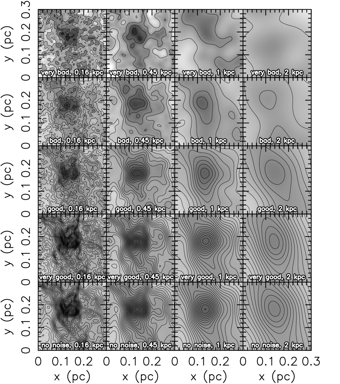
Figure 3.— Representations of the reference image as seen at four different angular resolutions (x axis) and five different noise levels (y axis). Each panel shows the same representative 0.3 pc $\times$ 0.3 pc section of the reference image. In each panel, the contours are spaced at intervals of 2$\sigma$ and they correspond to the contours used by clfind2d. Each image is shown as it would appear if observed with a 14″ circular beam from the distance shown in each panel. The noise levels are described in the text.

In nearby star-forming regions such as $\rho$ Oph and Orion, the typical size of presumed pre-protostellar cores is between 0.01 pc and 0.1 pc, with the average perhaps closer to 0.1 pc (Johnstone et al., 2000, 2001; Motte et al., 2001; Johnstone & Bally, 2006; Johnstone et al., 2006). Note that, although there is a lot of complex structure on the scale of pre-stellar cores in the simulated image at 0.16 kpc, all of this emission has been blended into a single object at 2 kpc. Observing this region from 2 kpc at a single wavelength, it would be impossible to know whether this was a single massive clump 0.2 pc across or a collection of unresolved smaller clumps.

Now we turn to the mass functions. The bottom row of Figure 4 shows the DCMFs for the clumps extracted from the convolved versions of the entire reference image. In each panel, the DCMF under study is compared to the reference DCMF from Figure 2 and the Salpeter power law. Clearly, coarsening the angular resolution depletes low-mass clumps in this no-noise case. However, no progressive shallowing of the mass function is observed. To make this point quantitatively, in Figure 5 we show the double power law which best fits each mass function. As shown in the figure, the exponent of the high-mass end of the power-law does not decrease systematically with increasing distance. At 0.16 kpc, it begins with a value of -2.8, somewhat lower than the nominal Salpeter value of -2.35, then drifts back and forth around a mean of -2.6 as the distance increases.

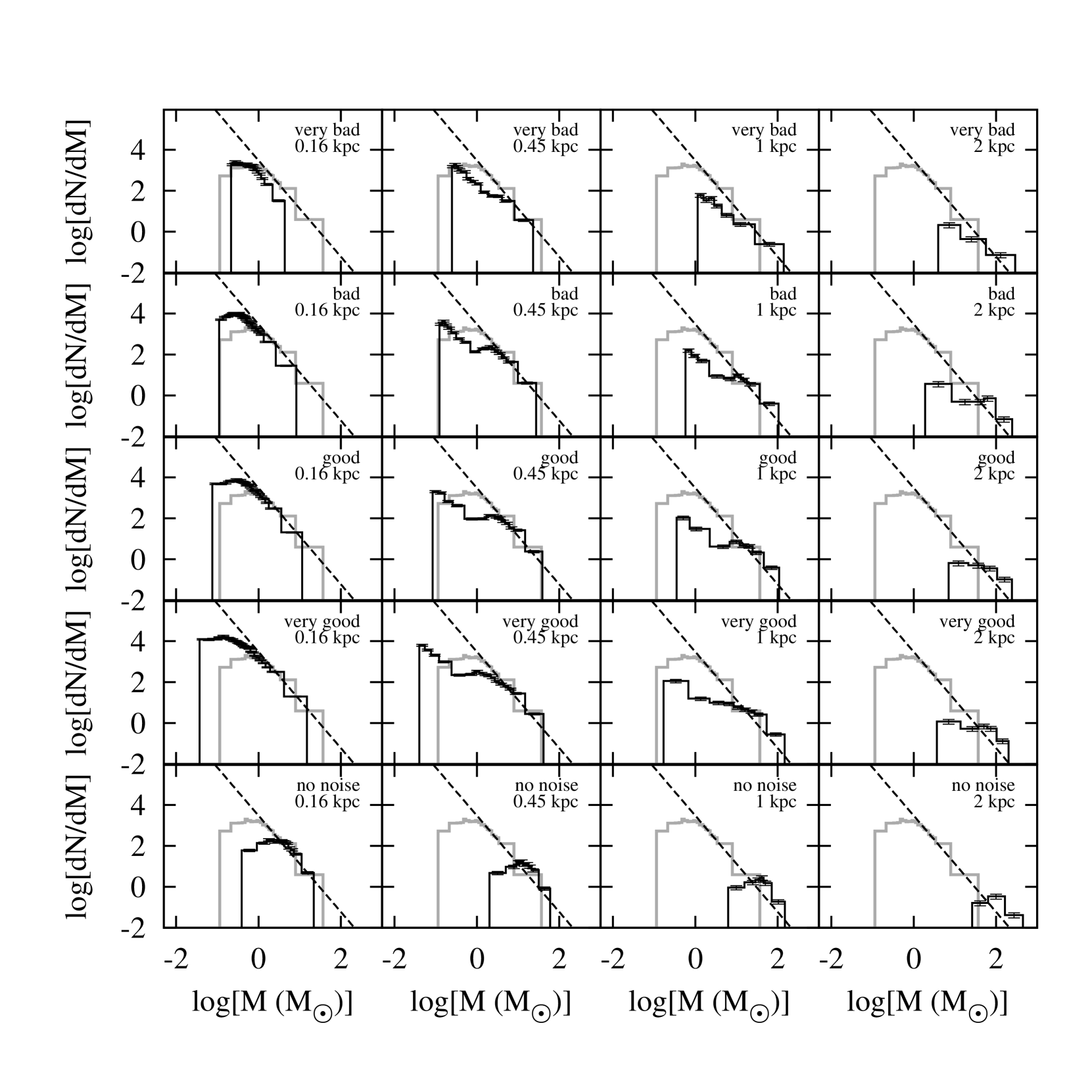
Figure 4.— Differential clump mass functions (black lines) extracted from versions of the reference image as convolved to the same resolutions and with the same levels of added noise as in Figure 3. Each DCMF is plotted over the DCMF of the clumps extracted from the reference image (grey line) as shown in Figure 2. The dashed line is the Salpeter mass function, which is shown in the same position in all of the panels to guide the eye.

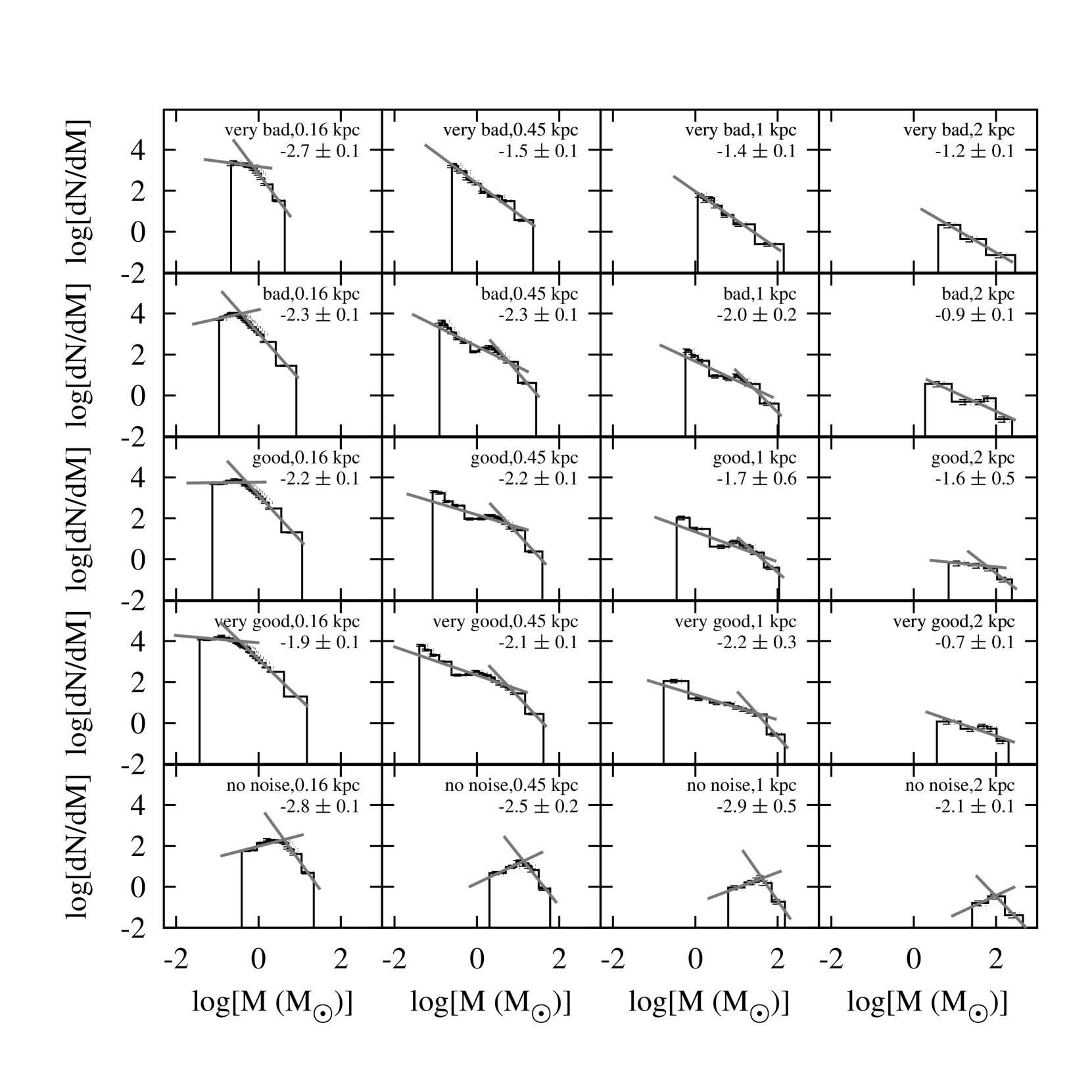
Figure 5.— Differential clump mass functions (black lines) as in Figure 4, but with power-law fits (gray lines). Each mass function is fit with the best-fitting double power law or, where a double power law did not produce a good fit, a single power law. The number indicated in the upper-right corner of each plot is the power-law index of either the single power law or the high-mass portion of the double power law.

Some of the changes in the mass function are obscured in the DCMF due to the decreasing total number of clumps. For this reason, we also plot, in Figure 6 the CCMFs for each image. The CCMF does not suffer from ambiguities due to binning: it shows every single clump in the data set. The Salpeter mass function is not drawn on these plots because, as described in Reid & Wilson (2006b), the Salpeter mass function does not have a simple power-law form on the CCMF if it is assumed to have one on the DCMF. Nevertheless, a similar result can be observed: in the no-noise case, there is no dramatic qualitative change in the shape of the CCMF as the resolution is coarsened.

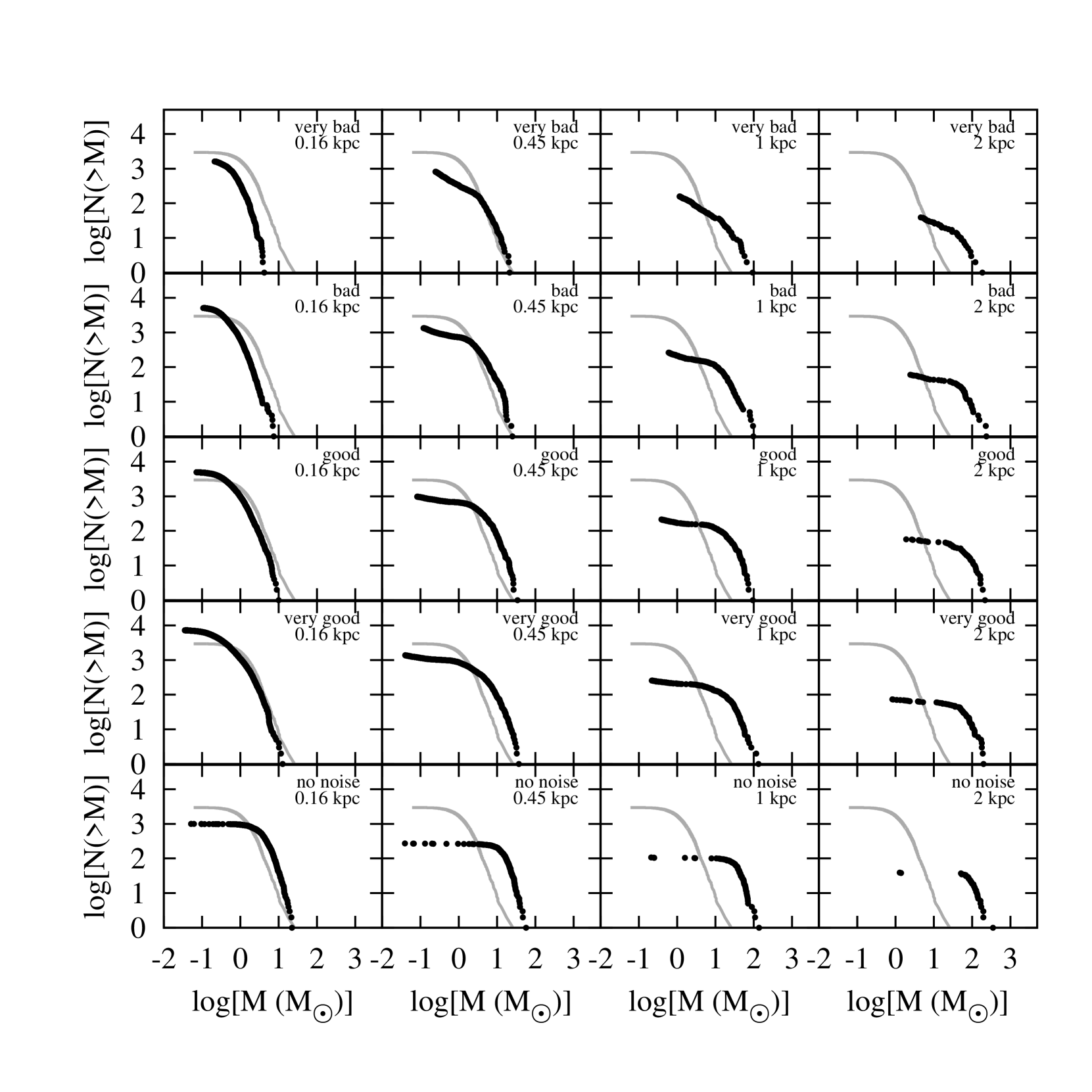
Figure 6.— Cumulative clump mass functions (black dots) extracted from versions of the reference image as convolved to the same resolutions and with the same levels of added noise as in Figure 3. Each CCMF is plotted over the CCMF of the clumps extracted from the reference image (grey line) as shown in Figure 2.

What should we make of the particular values of the power-law exponents obtained in the above fits? In their meta-analysis of the stellar IMF, (Kroupa, 2002) have shown that the slope of the high-mass end of the stellar IMF has a Salpeter-like mean of 2.36 with a standard deviation of 0.36. Thus, we may say that clump mass functions with power-law slopes in the range 2.0 to 2.7 are consistent with the stellar IMF within the measurement uncertainties. Within their uncertainties, all of the power-law fits to the no-noise DCMFs in Figure 5 would therefore seem to be consistent with the stellar IMF, although beyond the range usually interpreted to be so in studies of the clump mass function.

2.5. Noise Effects

In addition to finite angular resolution, real observations always have some level of noise, usually from both the sky and the instrument itself. Adding noise suppresses the detection of fainter clumps and changes the fluxes of all clumps. It must therefore affect the derived mass function. The properties of the noise in an image may depend strongly on the technique used to produce the image. For example, the scan-mapping technique common to most submillimeter cameras, including SCUBA (Holland et al., 1999) and SCUBA2 on the JCMT and both SPIRE and PACS on Herschel, tends to produce images with fairly smooth noise across most of the image and a region of high noise around the edge of the image where coverage is incomplete. Interferometer images, by contrast, typically have noise which is spatially very non-uniform. A single interferometric pointing results in noise which is low at the phase center but which climbs with distance from that center. In an interferometric mosaic, the noise pattern can be much more complicated.

For transparency and generality, we have adopted a simple prescription for adding noise to images. This technique most closely approximates the type of noise found in scan maps, which we argue are the type most commonly used in measuring the clump mass function and best suited for that purpose. We add Gaussian random noise on a per-pixel basis to the reference image and then convolve it with the beam, scaling the amplitude of the added noise appropriately so that it has the desired amplitude after convolution with the selected beam. This ensures that the noise in the image is correlated on angular scales matching the beam, as it is in real observations. To mimic a wide range of integration times and weather grades, we chose four representative noise levels which we label very good, good, bad, and very bad. Our “good” noise value, $\sigma_{\rm good}$, approximates the actual noise obtained in a typical 10′$\times$10′ SCUBA 850 $\mu$m scan map over 10 hours of integration in grade 2 weather (roughly 0.03 Jy beam^-1). The noise levels of the four grades differ by factors of 2, so that $\sigma_{\rm very\ good}=\sigma_{\rm good}/2=\sigma_{\rm bad}/4=\sigma_{\rm very\ bad}/8$. Modern instruments comparable to SCUBA, such as SCUBA2 and SPIRE, will typically produce images with less noise than our “good” level, but many archival observations will be closer to the “bad” noise level.

The noise-added versions of the reference image subsections discussed earlier are also included in Figure 3. Each row of the figure shows a different noise value. Scanning up a column shows the same subsection of the simulated region at a constant angular resolution but a progressively higher level of noise. Similarly, Figures 4, 5, and 6 show the DCMFs and CCMFs, respectively, of the reference image at each noise level and angular resolution.

Scanning up any given column in Figure 4 reveals that the effects of increased noise are most pronounced at low clump masses and near distances. Note that the addition of even a small amount of noise, as in the 0.16 kpc, very good noise image, increases the number of low mass clumps in the mass function. This occurs in part because the addition of noise raises some previously undetected peaks above the detection threshold, but also because noise can break apart more massive clumps, tricking clfind2d into thinking that they are multiple clumps of lower mass. This effect could be minimized in future by using multi-wavelength data sets in which each clump is observed independently more than once. Herschel will be very helpful in this regard.

However, note also that, at least in nearby regions, the addition of even substantial amounts of noise does not make the measured mass function conclusively non-Salpeter. This is evident from the fits in Figure 5 in which we see that most of the 0.16 kpc and 0.45 kpc mass functions are well fit by power laws whose exponents fall within the IMF-like range described in §2.4. Even at the higher distances of 1 kpc and 2 kpc, some of the mass functions retain this IMF-like shape. Referring back to Figure 3, we should be surprised by this result: the bad-noise images definitely do not all show the same population of objects, yet all but the 2 kpc versions are well fit by Salpeter-like power laws. The potentially worrisome conclusion is that even populations of clumps which are certainly not representative of pre-stellar objects may present Salpeter-like mass functions. If the clumps in the 0.16 kpc bad noise simulation are representative of pre-stellar clumps, surely the ones in the 1 kpc bad noise simulation are not, yet they are both well fit by mass functions which are compatible with the stellar IMF.

2.6. Chopping, Interferometry, and ‘Spatial Filtering’

Most measurements of the clump mass function made to date have been made from spatially filtered images. By “spatially filtered images”, we mean those which do not reproduce the emission from the source faithfully on all spatial scales. Instead, the source brightness is usually sampled on some finite set of spatial scales and then its image reconstructed using a Fourier-type method. Most often, this spatial filtering takes the form of chopping (Motte, André, & Neri, 1998; Johnstone et al., 2000, 2001; Motte et al., 2001; Reid & Wilson, 2005, 2006a) but it can also take the form of interferometry (e.g. Testi & Sargent 1998)

In chopped images, some of the flux from the source is lost. A full discussion of chopping and the common techniques for reconstructing images from chopped data can be found in Emerson (1995); Jenness et al. (1998), and Holland et al. (1999). Using a single chop throw is equivalent to multiplying the telescope’s spatial frequency response by a sine function, meaning that emission at all but a few spatial scales is attenuated to some degree (Emerson, 1995). A better strategy is to combine data sets made using several chop throws which have a small greatest common factor. In this way, the first null of the attenuating sine function can be made to correspond to angular scales much larger than any of interest in the image. Thus, the actual emission from the source can be reconstructed with high fidelity (or perfect fidelity, in the limit of no noise). Clump mass functions produced from images acquired in this way should be relatively unaffected by the spatial filtering.

Interferometric observations are typically more strongly filtered than chopped images, so the effect on the clump mass function of this filtering may be more pronounced and harder to predict. Like chopped images, interferometric images only include emission from the source on certain ranges of spatial scales. Optimizing for high angular resolution typically sacrifices emission on large spatial scales. Modern interferometers with many elements attempt to maximize both angular resolution and sensitivity to a broad range of spatial scales. For example, ALMA will incorporate the smaller Atacama Compact Array (ACA), which will improve its sensitivity to emission on large spatial scales.

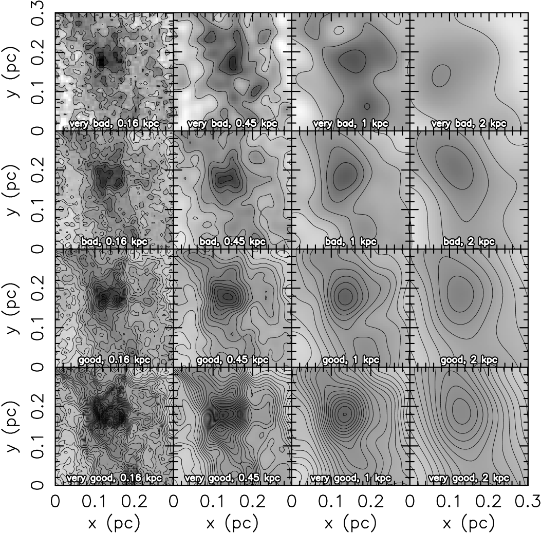
Figure 7.— Representations of the chopped versions of the reference image as seen at four different angular resolutions (x axis) and four different noise levels (y axis). The areas covered and the contour levels used are identical to those in Figure 3. Note that there is no noise-free version of each image because, in the limit of no noise, a chopped image is identical to the original.

Rather than attempting to simulate many specific cases of spatial filtering, we have chosen two generic representations: a common type of chopping and a moderate form of interferometric filtering. In the first, we simulate a chopped image taken with three chop throws. We chose the recommended minimum of three chop throws with no large common factor , in this case 30″, 44″, and 68″. Figure 7 shows the same subsections of the reference image as Figure 3, but with chopping applied. The corresponding clump mass functions are compared with the reference mass function in Figure 8 and shown with best-fitting power laws in Figure 9. Note that there is no noise-free case shown in these figures as, in the absence of the noise, a chopped image is identical to the original so that the no-noise results in this case would be the same as in the bottom row of Figure 4.

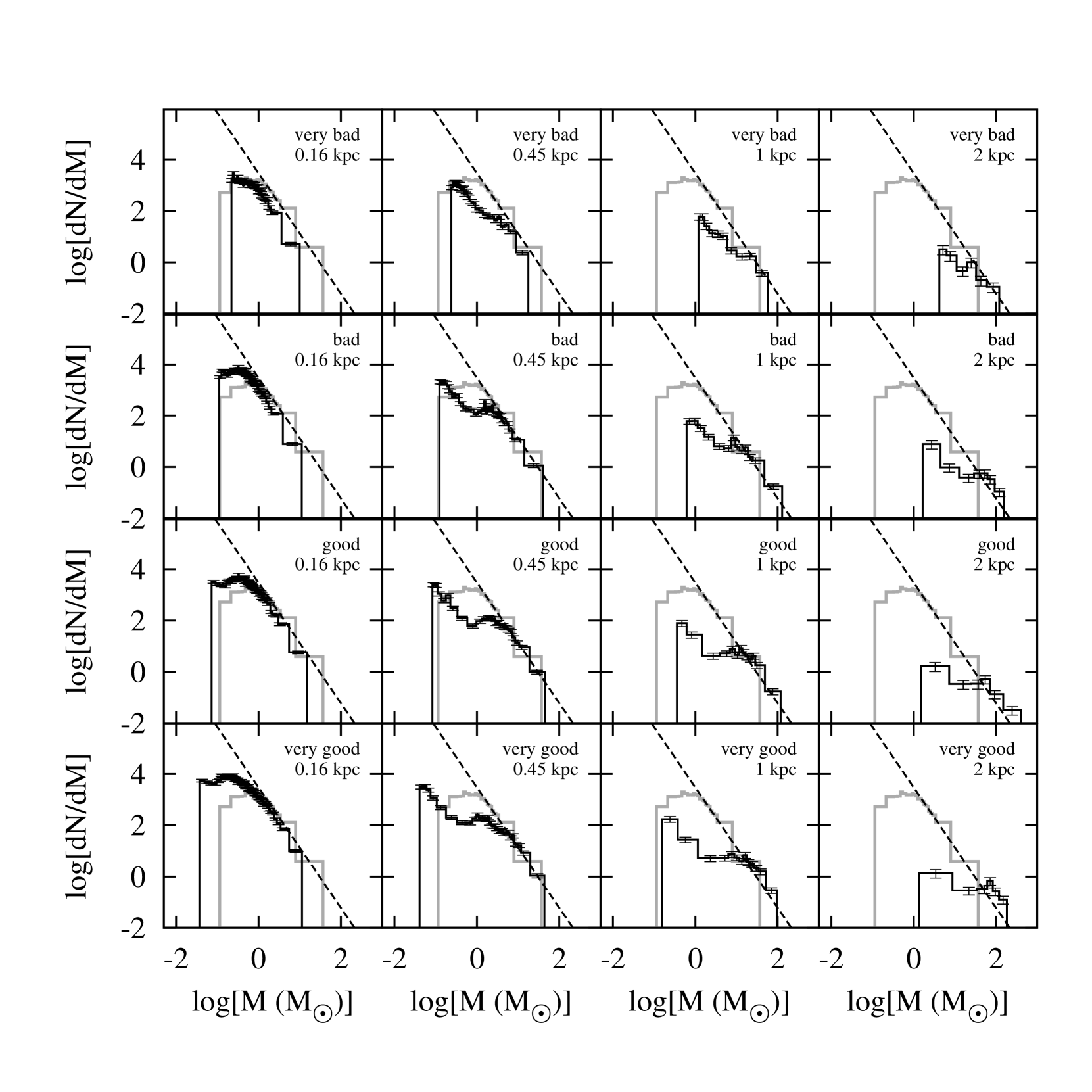
Figure 8.— Differential clump mass functions (black lines) extracted from the chopped versions of the reference image. The angular resolutions and noise levels are as described in Figure 4, but for the lack of the no-noise versions. Each DCMF is plotted over the DCMF of the clumps extracted from the reference image (grey line) as shown in Figure 2. The dashed line is the Salpeter mass function, which is shown in the same position in all of the panels to guide the eye.

Figure 9.— Differential clump mass functions (black lines) as in Figure 8, but with power-law fits (gray lines). Each mass function is fit with the best-fitting double power law or, where a double power law did not produce a good fit, a single power law. The number indicated in the upper-right corner of each plot is the power-law index of either the single power law or the high-mass portion of the double power law.

Comparison of Figures 8 and 4 shows that, as expected, the clump mass functions do not change much due to chopping, as long as a sufficient number of chop throws with a small greatest common factor are used (three suffices).

The same cannot be said of mass functions measured from more heavily filtered images, such as those produced through interferometry. We simulate the effects of interferometric spatial filtering in a general way not tied to any particular instrument. We choose to suppress emission on scales larger than about 2′. To do so, we multiply the Fourier transform of the image by a circularly symmetric Gaussian whose full-width at half maximum corresponds to angular scales of 2′in the image plane. Our choice of a Gaussian taper with this width is somewhat arbitrary: different tapering functions with different widths would correspond to different interferometer configurations. We performed many such manipulations of the image but, as the essential results do not change, we present only this set for brevity.

Figure 10.— Representations of the versions of the reference image as seen at four different angular resolutions (x axis) and four different noise levels (y axis), but with emission on scales larger than 2′ strongly suppressed to mimic interferometric observations. The areas covered and the contour levels used are identical to those in Figure 3.

Figure 11.— Differential clump mass functions (black lines) extracted from the versions of the reference image in which emission on spatial scales larger than 2′ has been strongly suppressed. The angular resolutions and noise levels are as described in Figure 4. Each DCMF is plotted over the DCMF of the clumps extracted from the reference image (grey line) as shown in Figure 2. The dashed line is the Salpeter mass function, which is shown in the same position in all of the panels to guide the eye.

Figure 12.— Differential clump mass functions (black lines) as in Figure 11, but with power-law fits (gray lines). Each mass function is fit with the best-fitting double power law or, where a double power law did not produce a good fit, a single power law. The number indicated in the upper-right corner of each plot is the power-law index of either the single power law or the high-mass portion of the double power law.

As before, Figure 10 shows the standard subsection of the reference image, now filtered. Figure 11 shows the corresponding DCMFs compared to the reference mass DCMF and Figure 12 shows the DCMFs fitted with double power laws.

These heavily spatially filtered images produce a marked change in the clump mass function. They demonstrate how difficult it can be to predict the effect on the clump mass function of different types of image acquisition techniques. In the 0.16 kpc maps with bad and very bad noise, all of the clumps have fallen below the detection threshold. This again reminds us that the threshold for detection of clumps is a surface brightness, not an absolute flux. Because these two simulated regions are nearby, the emission from their clumps occurs on relatively large angular scales, so they are filtered out by the simulated interferometry. Thus, as Figure 11 shows, the DCMFs of the nearer regions are actually less similar to that of the reference DCMF than are those of the more distant regions. Measurements of the clump mass function with interferometers such as ALMA must take this effect into account.

The shape of the mass function is strongly affected by interferometry. In several cases, double power law fits now simply converge to single power laws; in those cases, we show the single power law and its exponent in Figure 12. Interferometry does us the favor of removing distracting emission from the diffuse background which is probably not directly involved in star formation. Consulting Figure 10, we can see that the clumps are much more visible than in Figure 3. Perhaps as a result, the mass functions in Figure 10 are now consistently shallower than the Salpeter IMF. Yet still there are cases where, although the images themselves show that the population of clumps has changed substantially due to noise, resolution, and filtering effects, the mass function is well-fit by a Salpeter-like power law. Again, it appears that even when the objects from which the clump mass function is made are not themselves the precursors of individual stars, the mass function may appear Salpeter-like.

2.7. Implications for Measurements of the Clump Mass Function

What are the consequences of these results for measurements of the clump mass function? In attempts thus far to measure the clump mass function and compare it to the stellar IMF, the comparison has often been framed in this form: “Does this mass function look like a Salpeter power-law?” However, we have shown that there are many cases in which a population of objects–poorly resolved, noisy blobs derived from observations of star-forming regions–may yield Salpeter-like mass functions. Hence, we suggest that a better question would be “Do I have reason to believe that my observations would not yield a Salpeter-like mass function?” If the observations cannot be expected a priori to definitively discriminate between Salpeter and non-Salpeter forms, then any resulting appearance of a Salpeter-like clump mass function should not be over-interpreted.

Our best prospects for measuring the clump mass function accurately rest with single-dish telescopes, where spatial filtering can be minimized and sensitivity maximized over a large field of view. Herschel and SCUBA2 promise to be a powerful combination in this regard because both have achieved unprecedented sensitivity in their respective wavebands and they have complementary resolving power: where Herschel is unable to resolve individual pre-stellar cores at long wavelengths, SCUBA2 will provide the required resolving power.

In interpreting clump mass functions produced from single-dish observations, readers should remember that having a Salpeter-like mass function is not conclusive evidence that a population of clumps represent individual pre-stellar cores. Rather, the argument should be approached from the opposite direction: do these objects that I know are pre-stellar cores (by other lines of evidence), have a Salpeter-like mass function?

2.8. Characteristic Scales of the Mass Function and the Star Formation Efficiency

Some authors have noted that the characteristic mass scales of the stellar IMF and clump mass functions seem to match, modulo some star formation efficiency (e.g. Johnstone et al. 2000, 2001; Motte et al. 2001, 2007). The idea is that one can obtain the stellar IMF from the clump mass function by multiplying the masses of all of the clumps by some star formation efficiency less than unity. To derive this efficiency, one can compute the ratio of certain characteristic masses measured from both mass functions. The clump mass function has two basic characteristic masses: the “peak” or “turnover” mass, which is simply the mass at which the mass function peaks, and the “break mass”, which is the break point between the two power laws when the mass function is fit with a double power law. The break mass is equal to or greater than the peak mass. One can compute a star formation efficiency from either value. For example, if the break mass in the stellar IMF were 0.3 M_⊙ and that in the mass function of pre-stellar cores were 3 M_⊙  one might conclude that the star formation efficiency was about 10%.

Figure 13.— Break mass versus distance to various observed and simulated star-forming regions. The break mass is a parameter of a double power law fit to a clump mass function and represents the mass at which the two power laws intersect. Break masses from the observational data are shown with filled circles, while those from the simulations with no noise and good noise are shown with filled triangles and squares, respectively. The lines of best fit shown are power laws in distance with exponents of 1.2 for the noise-free simulations (solid line) and 1.8 for both the simulations with good noise (dotted line) and the observations (dashed line).

However, this interpretation of these results may also be too simplistic. Scanning across any row in figure 5 demonstrates that, as distance increases, both the peak and break masses also increase. In effect, the whole mass function shifts to higher masses. To make this point explicit, we plot in Figure 13 the fitted DCMF break mass versus the distance to several star-forming regions, both simulated and real. The real data come from fits to the mass functions of the following star-forming regions, in order of increasing distance: $\rho$ Oph (Johnstone et al., 2000; Motte, André, & Neri, 1998), Orion B (Johnstone et al., 2001; Motte et al., 2001), M8 (Tothill et al., 2002), Cygnus X (Motte et al., 2007) (using data read from their published graphs), M17 (Reid & Wilson, 2006a), and NGC 7538 (Reid & Wilson, 2005). For M8 and M17, we have used the revised distance estimates of 1.3 kpc (Tothill et al., 2008) and 2.1 kpc (Chini & Hoffmeister, 2008).

Fitting the simulated data with no noise and good noise, we find that the break mass scales with distance as $d^{1.2}$ and $d^{1.8}$, respectively. Fitting the data derived from actual observations, we find that the break mass scales with distance again as $d^{1.8}$. The simulations produce consistently higher break masses than do the observations. We cannot account quantitatively for this result yet, but we suspect it results from the much larger areal coverage (and hence larger number of clumps) in the simulations than in the observations. Having more clumps in the sample may increase the statistical weight of the high-mass end of the mass function, where the statistics within the observations are usually poor (because higher mass clumps are rarer).

Unlike the simulated images, which differ only in the distance to the simulated region, the observational data sets differ widely in the telescope used to acquire the data, the wavelength at which the data were acquired, and the clump-finding algorithm used to extract the clumps. As we mentioned in §2.1, this supports the argument that the properties of derived clump mass functions do not depend strongly on the choice of clump-finding algorithm.

That the break mass should scale with the distance to the region being observed is exactly what one would expect if the break mass were not a property of the ensemble of clumps themselves, but a function of the angular resolution at which they are observed. If the break mass reflected, say, the local Jeans mass or some property of turbulence, it ought not to scale with the distance to the observed region if the all regions were observed with sufficiently high angular resolution.

This scaling of the break mass with distance is already implicit in other results in the literature. For example, Motte et al. (2007) showed that, in the massive star-forming complex Cygnus X, which lies at a distance of 1.7 kpc, the typical volume-averaged density of a clump is about an order of magnitude lower than that of the clumps in $\rho$ Oph, which lies at only 0.16 kpc. This could as easily be a resolution effect as a physical one.

If the characteristic masses of the clump mass functions observed to date really are set more by the distances to the regions observed than by the physics of the material within those regions, then their use in deriving star formation efficiencies must be questioned. Herschel and SCUBA2 will both offer observations with improved angular resolution and sensitivity, allowing us to test the robustness of this distance scaling.

3. The Lognormal Mass Function

We showed in §2.5 that, even when a population of clumps has been distorted beyond recognition by noise and coarse angular resolution, its mass function may still be consistent with the stellar IMF within the uncertainties. We believe that this behavior of the clump mass function reflects the deeper origins of the shape of the clump and stellar mass functions.

The stellar IMF is frequently described as a Salpeter-like power-law. This interpretation is somewhat outdated; it reflects the limited range of stellar masses included in Salpeter’s original stellar IMF. More recent measurements of the stellar IMF show that, when it is extended to low stellar masses, well below the turnover mass, it adopts a lognormal form (Chabrier, 2003), sometimes approximated by four or five power-law segments of which the Salpeter power-law is but one. The Salpeter power law appears merely to be a good approximation to the lognormal IMF over a restricted range of stellar masses, perhaps 1–10 M_⊙.

Several authors have shown that a lognormal stellar IMF arises naturally as a consequence of the Central Limit Theorem of calculus (Larson, 1973; Zinnecker, 1984; Adams & Fatuzzo, 1996). When a sufficiently large number of independent physical processes or variables act together to produce the stellar IMF, it naturally tends towards a lognormal form. The larger the number of independent variables used in models of the origin of the IMF, the more closely the IMF approaches the lognormal form (Adams & Fatuzzo, 1996).

The same reasoning applies to the clump mass function for two reasons: first, a large number of independent factors must act to set the distribution of clump masses and, second, it is that distribution of clump masses which must ultimately give rise to the IMF. Reid & Wilson (2006b) showed that clump mass functions measured from dust continuum maps are typically well fit by lognormal functions. This result holds true despite the large variety of different methods of acquiring the data and extracting the clumps used in producing the various mass functions. In Figure 14, we show that the mass functions first shown in Figure 4 are all well fit by lognormal distributions. This is easier to see when plotting CCMFs, which show every clump in the sample. A lognormal DCMF corresponds to an error function. We believe that the high quality of the lognormal fits to the simulated clump mass functions suggest that they, too, are being biased toward this form by the cumulative action of a large number of independent processes. These factors need not be physical processes, as assumed in models of the origin of the stellar IMF. The independent processes might equally well include those discussed in §2.1, namely things like the addition of random amounts of noise to each clump, random errors in the assignment of clump boundaries by clump-finding algorithms, and the perturbations to each clump’s mass caused by convolution with other clumps and superposition along the line of sight. Indeed, as the plots in Figure 14 show, the combined effects of large amounts of noise and very coarse angular resolution do not ruin the lognormal shape of the mass function.

Figure 14.— Cumulative clump mass functions (black dots) identical to those in Figure 6, including the mass function of the reference image (grey line), but adding a fitted error function (red line). The error function is the CCMF equivalent of a lognormal DCMF.

Our reference mass function already has a lognormal form. The only post-processing required to construct that mass function was the use of a clump-finding algorithm; excessive noise and coarse angular resolution are not factors. Adding noise and coarsening the resolution of the simulation appears to change the width and normalization of the lognormal clump mass function, but not to make it any less lognormal. This is the behavior one expects if the Central Limit Theorem is setting the clump mass function. However, it raises the prospect that it may be very difficult indeed to measure a clump mass function which is not lognormal. If all clump mass functions appear lognormal, it may be difficult to distinguish those whose width and normalization were set by the physics of star formation and those whose characteristics were set by our data acquisition and analysis techniques.

4. Conclusions

We have investigated the effects on the derived clump mass function of image noise, image angular resolution, and two kinds of spatial filtering. We have found that adding noise to an image and coarsening its resolution to the point where the objects in the image are clearly no longer the precursors of individual stars frequently does not cause its mass function to become incompatible with the Salpeter stellar IMF. When the simulated mass functions are fit with power laws, the distribution of the power law exponents caused by noise and degraded resolution mirrors the distribution of measured exponents in the stellar IMF. The clump mass function only deviates conclusively from the Salpeter form when it is derived from heavily spatially filtered observations.

Following other authors (Larson, 1973; Zinnecker, 1984; Adams & Fatuzzo, 1996), we have suggested that the clump mass function has a lognormal form due to the cumulative action of many independent processes in determining the mass of any given clump. We have extended the set of such possible processes to encompass not only physical processes occurring in star-forming regions, but the processes of data acquisition and analysis. The cumulative action of factors such as turbulence, temperature variations, radiative effects, numerous uncertainties in our conversion of flux to mass, our clump-finding algorithms, image noise, source blending, and spatial filtering may ensure that clump mass functions always appear lognormal. The Salpeter-like appearance of their high-mass ends may simply reflect this lognormal form.

Collectively, these results suggest that we ought to adopt a skeptical approach when interpreting the clump mass function. We cannot conclude that, because the mass function of a set of clumps has a Salpeter-like form, those clumps represent the precursors of individual stars. We may be able to draw this conclusion in the very limited set of cases in which our observations have very little noise and sufficient resolution to distinguish individual pre-stellar cores. Dust continuum maps made with Herschel’s PACS instrument have a lot of promise in this regard because they have unparalleled sensitivity and resolution. However, we will demonstrate in a forthcoming paper that even clump mass functions derived from PACS maps can show a convincing Salpeter-like form in cases where we do not believe the constituent clumps to be pre-stellar cores.

The study of the origin of the stellar IMF is important to many areas of astronomy. It is worth very careful scrutiny. We suggest that the best measurements of the clump mass function with the current generation of instruments will come from a combination of PACS and SCUBA2 data. High-sensitivity, multi-wavelength observations at high spatial resolution will allow us to reduce the effects of many of the uncertainties discussed in this paper. Using the multi-wavelength data, we will be able to better constrain the temperatures and dust opacities of the clumps, improving our estimates of their masses. Using Spitzer and PACS data, we will be able to do a better job of filtering out cores which are already forming stars. Follow-up observations to obtain high-resolution molecular line data will further allow for the exclusion of clumps which are not gravitationally bound, as well as limited deconvolution of the emission along the line of sight.

The comparison of Herschel and SCUBA2 clump catalogs for matching regions will be highly instructive. Such a comparison would allow us to assess, in a quantitative and statistically significant way, whether our measurements of the masses of individual clumps are robust. If, for example, both SCUBA2 and Herschel generate Salpeter-like mass functions, but with very different masses for each individual clump, this will be good evidence for our argument that the shape of the clump mass function can be set by non-physical means. We will be very reassured if the two clump catalogs contain similar objects with similar masses (or fluxes).

In the more distant future, the Cornell Caltech Atacama Telescope (CCAT, Sebring et al. 2006) promises to be a powerful tool for measuring the clump mass function. As a single-dish telescope, it will not suffer the spatial filtering effects that may make its contemporary, the Atacama Large Millimeter Array, less useful for measuring the clump mass function. With an expected dish diameter of 25 m, CCAT’s angular resolution of 2″ at 200 $\mu$m will make it a powerful clump-finding tool.

References

- Adams & Fatuzzo (1996) Adams, F. C., & Fatuzzo, M. 1996, ApJ, 464, 256
- Alves, Lombardi, & Lada (2007) Alves, J., Lombardi, M., & Lada, C. J. 2007, A&A, 462, L17
- Bate et al. (2003) Bate, M. R., Bonnell, I. A., & Bromm, V. 2003, MNRAS, 339, 577
- Chabrier (2003) Chabrier, G. 2003, PASP, 115, 763
- Chini & Hoffmeister (2008) Chini, R. & Hoffmeister, V. 2008, in Handbook of Star Forming Regions, Volume II: The Southern Sky ASP Monograph Publications, Vol. 5., ed. B. Reipurth, 625
- Curtis & Richer (2010) Curtis, E. I., & Richer, J. S. 2010, MNRAS, 402, 603
- Emerson (1995) Emerson, D. T. 1995, in Multi-feed systems for radio telescopes, Eds. Emerson D.T. & Payne J.M., ASP Conf. Ser. 75, 327
- Griffin et al. (2009) Griffin, M., et al. 2009, in EAS Publication Series 34, ed L. Pagani & M. Gerin, 33
- Holland et al. (1999) Holland, W. S., et. al. 1999, MNRAS, 303, 659
- Johnstone et al. (2000) Johnstone, D. J., Wilson, C. D., Moriarty-Schieven, G., Joncas, G., Smith, G., Gregersen, E., & Fich, M. 2000, ApJ, 545, 327
- Johnstone et al. (2001) Johnstone, D. J., Fich, M., Mitchell, G. F., & Moriarty-Schieven, G. 2001, ApJ, 559, 307
- Johnstone & Bally (2006) Johnstone, D. J. & Bally, J. 2006, ApJ, 653, 383
- Johnstone et al. (2006) Johnstone, D. J., Matthews, H., & Mitchell, G. F. 2006, ApJ, 639, 259
- Jenness et al. (1998) Jenness, T., Lightfoot, J. F., & Holland, W. S. 1998, Proc. SPIE 3357, 548
- Kauffmann et al. (2010) Kauffmann, J., Pillai, T., Shetty, R., Myers, P. C., & Goodman, A. A. 2010, ApJ, 716, 433
- Kramer et al. (1998) Kramer, C., Stutzki, J., Röhrig, R., & Corneliussen, U. 1998, A&A, 329, 249
- Kroupa (2002) Kroupa, P. 2002, Science, 295, 82
- Larson (1973) Larson, R .B. 1973, MNRAS, 161, 133
- Maíz-Apellániz & Úbeda (2005) Maíz-Apellániz, J. & Úbeda L. 2005, ApJ, 629, 873
- Motte et al. (2001) Motte, F., André, P., Ward-Thompson, D., & Bontemps, S. 2001, A&A, 372, L41
- Motte et al. (2007) Motte, F., Bontemps, S., Schilke, P., Schneider, N., Menten, K. M., & Broguière, D. 2007, A&A, 476, 1243
- Motte, André, & Neri (1998) Motte, F., André, P., & Neri, R. 1998, A&A, 336, 150
- Petitclerc (2009) Petitclerc, N. 2009, Ph.D. Thesis
- Pineda, Rosolowsky, & Goodman (2009) Pineda, J. E., Rosolowsky, E. W., & Goodman, A. A. 2009, ApJ, 699, L134
- Poglitsch & Altieri (2009) Poglitsch, A. & Altieri, B. 2009, in EAS Publication Series 34, ed L. Pagani & M. Gerin, 43
- Reid & Wilson (2005) Reid, M. A., & Wilson, C. D. 2005, ApJ, 625, 891
- Reid & Wilson (2006a) Reid, M. A., & Wilson, C. D. 2006, ApJ, 644, 990
- Reid & Wilson (2006b) Reid, M. A., & Wilson, C. D. 2006, ApJ, 650, 970
- Robson & Holland (2007) Robson, I., & Holland, W. 2007, in ASP Conf. Ser. 375, From Z-Machines to ALMA: (Sub)Millimeter Spectroscopy of Galaxies, ed. A. J. Baker, J. Glenn, A. I. Harris, J. G. Mangum, & M. S. Yun, 275
- Rosolowsky et al. (2008) Rosolowsky, E. W., Pineda, J. E., Kauffmann, J., & Goodman, A. A. 2008, ApJ, 679, 1338
- Salpeter (1955) Salpeter, E. E. 1955, ApJ, 121, 161
- Sebring et al. (2006) Sebring, T. A., Giovanelli, R., Radford, S., & Zmuidzinas, J. 2006, in SPIE Conf. Ser. 6267, Ground-based and Airborne Telescopes, ed. L. M. Stepp, 62672C
- Stutzki & Guesten (1990) Stutzki, J., & Guesten, R. 1990, ApJ, 356, 513
- Testi & Sargent (1998) Testi, L. & Sargent, A. I. 1998, ApJ, 508, L91
- Tothill et al. (2002) Tothill, N. F. H., White, G. J., Matthews, H. E., McCutcheon, W. H., McCaughrean, M. J., Kenworthy, M. A. 2002, ApJ, 580, 285
- Tothill et al. (2008) Tothill, N. F. H., Gagné, M., Stecklum, B., & Kenworthy, M. A. 2008, in Handbook of Star Forming Regions, Volume II: The Southern Sky ASP Monograph Publications, Vol. 5., ed. B. Reipurth, 533
- Wadsley et al. (2004) Wadsley, J. W., Stadel, J., & Quinn, T. 2004, New Astronomy, 9, 137
- Williams, de Geus, & Blitz (1994) Williams, J. P., de Geus, E. J., & Blitz, L. 1994, ApJ, 428, 693
- Zinnecker (1984) Zinnecker, H. 1984, MNRAS, 210, 43