Impact of network structure on a model of diffusion and competitive interaction

Abstract

We consider a model in which agents of different species move over a complex network, are subject to reproduction and compete for resources. The complementary roles of competition and diffusion produce a variety of fixed points, whose stability depends on the structure of the underlying complex network. The survival and death of species is influenced by the network degree distribution, clustering, degree-degree correlations and community structures. We found that the invasion of all the nodes by just one species is possible only in Erdös–Renyi and regular graphs, while networks with scale–free degree distribution, as those observed in real social, biological and technological systems, guarantee the co–existence of different species and therefore help enhancing species diversity.

In the last few years, complex networks have been the subject of an increasingly large interest in the scientific community rev1 ; rev2 ; rev3 . This is due to: i) the wide variety of complex systems that can be described as graphs with a complex topology; ii) the recent observation that various dynamical processes taking place on networks, such as epidemics epidemics , random walks noh04 ; brw , synchronisation arenas and self–organised criticality moreno ; JensenBook , can be affected by the underlying network structure. Concerning social interactions, many models have been proposed in the last decades to study evolution of relationships, culture segregation, opinion formation and propagation of new ideas by means of majority rules, melting or mixing, and have also been studied on complex topologies Jensen01 ; Jensen02 ; Schelling ; Axelrod ; Castellano . Particularly important contributions to the understanding of social dynamics taking place on networks have been provided by evolutionary game theory hs ; nowak . Usually, when an evolutionary game is studied on a graph, each individual is associated to a node of the graph, and the social relationships are represented by the links. Individuals interact with their neighbours on the graph by playing various evolutionary games, and different collective behaviours emerge, such as global cooperation or selfishness, according to the structure of the underlying network of relationships santos ; game1 . These models on complex networks fail to catch one of the most important characteristic of real evolutionary systems, namely the possibility for the individuals to move through a complex environment and to interact with a neighbourhood which changes over time tang . Some recent works have proposed extensions of evolutionary game theory to moving agents Helbing2 ; Meloni . In these latter models, the individuals move over a continuous space or a discrete lattice, and play games with other individuals in their spatial neighbourhood. However, the hypothesis of a homogeneous and continuous space is too simplistic, and does not correspond to the structure of real social and technological networks rev1 ; rev2 ; rev3 ; airplane . Metapopulation models with heterogeneous connectivity patterns, which incorporate mobility over the nodes, local interaction at the nodes, and a complex network structure, have been recently proposed only in specific contexts such as epidemic spreading  eubank or chemical reactions  Colizza2 . In this Letter we propose and study a simple and general model of evolution of species over a complex network. In the model, each species can represent either a biotype or a language, a culture or even a consumer product. The species compete for space or resources, represented by the nodes of the network. For instance, if the species are consumer products, each node is a potential user and the species move from node to node through the network of social relationships among users, competing to be adopted by as many users as possible. Instead, if we imagine each species as a different biotype, the complex network represents the connections among spatial environments, and species compete for food or energy. The agents of different species move over the graph by diffusion and their interaction at the nodes is modelled by means of competition and replication rules. The aim of the present work is to study the combined effects of diffusion over a complex topology and of competitive selection at nodes. Notice that whenever we refer to selection in the following, we always intend competitive selection, i.e. competition for resources among the different species at the same node. As we will show in the following, the model, although extremely simple, is rich enough to exhibit a large variety of patterns over time and a final distribution of the species that is intrinsically connected with the structure of the network.

Let us consider a connected graph with $N$ nodes and $K$ links, described by an adjacency matrix $A=\{a_{ij}\}$, and a population of $N_{s}$ different species, labelled by the index $\alpha=1,2,\ldots,N_{s}$. Each node of the graph is an environmental niche which can host individuals of one or more species, and the links represent connections between niches. At every single node of the graph, there is room for each of the $N_{s}$ species. We denote with $P_{i}^{\alpha}(t)$ the relative abundance of the $\alpha$-th species at node $i$ at time $t$. Such abundances are normalised so that all nodes have the same capacity, i.e. $\sum_{\alpha}P_{i}^{\alpha}(t)=1,\forall i,t$. We denote with $P^{\alpha}(t)=\sum_{i}P_{i}^{\alpha}(t)$ the overall abundance of species $\alpha$ in the network, so that $\sum_{\alpha}P^{\alpha}(t)=N$. At each time step, the model considers two different processes, namely diffusion and competition. In the diffusion process, a fraction $p$ ($0\leqslant p\leqslant 1$) of the individuals which are at a given node $j$ move to one of the first neighbours of $j$, let us say $i$, with a uniform probability: $\frac{a_{ji}}{\sum_{l}a_{jl}}$. The remaining fraction $1-p$ stays at node $j$. After the diffusion process, the selection process takes place, which normalises the number of individuals at each node in order to guarantee that $\sum_{\alpha}P_{i}^{\alpha}(t)=1,\forall i,t$. The survival and death of individuals at each node is governed by a generalised replicator dynamics hs ; nowak . In its simplest version, which takes into account an ecosystem with only two species, say $X$ and $Y$, the equations of the replicator dynamics read:

$$\begin{split}x(t+1)=\dfrac{f[x(t)]}{\phi}x(t),&\quad y(t+1)=\dfrac{g[y(t)]}{\phi}y(t)\end{split}.$$ (1)

where $x(t)$ and $y(t)$ denote the percentages of individuals of species $X$ and $Y$ at time $t$, respectively, while $f[x(t)]$ and $g[y(t)]$ are two functions which measure the fitness of each of the two species. The interaction between $X$ and $Y$ is ruled by the quantity $\phi$, which plays the role of an environmental limit and is fixed to ensure the normalisation $x(t)+y(t)=1~{}\forall t$. This gives $\phi=xf(x)+yg(y)$, so that $\phi=\phi(x,y)$ is the average fitness of the population. The meaning of Eq. (1) is the following: when the only constraint imposed to the species evolution is the environmental limit $\phi$, their relative abundance at the next time step will increase or decrease according to their fitness. As for the fitness functions $f(x)$ and $g(y)$ we consider the general case nowak $f(x)=b_{x}x^{\gamma-1}$ and $g(y)=b_{y}y^{\gamma-1}$ where $b_{x}>0$, $b_{y}>0$, and the exponent $\gamma$ is a real number that can be varied to tune the dependence of the fitness function of a species on its abundance. The fixed points $(x^{*},y^{*})$ of Eq. (1), and their stability, depend on the value of $\gamma$. We distinguish three cases: $\gamma$ smaller, equal or larger than $1$. For $\gamma<1$ there are two unstable fixed points $(1,0)$ and $(0,1)$, and one stable fixed point $x^{*}=(1+(b_{x}/b_{y})^{\frac{1}{\gamma-1}})^{-1}$, $y^{*}=1-x^{*}$. The two species $X$ and $Y$ will coexist despite their initial relative abundances and fitness. This case is called survival for all. If $\gamma=1$, there are only two fixed points whose stability depends on the respective values of $b_{x}$ and $b_{y}$. When $b_{x}>b_{y}$ then $(1,0)$ is stable while $(0,1)$ is unstable, conversely when $b_{x}<b_{y}$, $(0,1)$ is a stable equilibrium while $(1,0)$ in unstable. Independently of the initial distributions of the two species, if $b_{x}>b_{y}$ then $x$ will eventually overcome $y$ until all individuals of species $y$ are extinct. This case is called survival of the fittest. Finally, for $\gamma>1$ the third fixed point is unstable, while $(1,0)$ and $(0,1)$ are both stable. In particular if the initial condition $x(0)$ is such that $x(0)>x^{*}$, then $x(t)$ will eventually overcome $y(t)$, independently of the value of $b_{x}$ and $b_{y}$, while $y(t)$ will overcome $x(t)$ if $x(0)<x^{*}$ (notice that $x^{*}=1/2$ when $b_{x}=b_{y}$). This super-exponential growth always guarantees the survival (and reproduction) of the most abundant species, so that the case $\gamma>1$ is usually called survival of the first. In order to implement a strong competition among species at a node, in the following we always consider $\gamma>1$. The replicator dynamic can be easily extended to $N_{s}$ different species. A super-exponential growth is predicted for the $N_{s}$-dimensional replicator equations when $\gamma>1$, and all the corners of the $N_{s}$-dimensional simplex are stable fixed points. We consider a fitness function of the form $f(P_{i}^{\alpha})=b_{i}^{\alpha}(P_{i}^{\alpha})^{\gamma-1}$, where $\gamma>1$ and, without any lack of generality, we set $b_{i}^{\alpha}=1$ $\forall i$ and $\forall\alpha$. In fact, when $\gamma>1$ only the most abundant species will survive, despite the relative values of $b_{i}^{\alpha}$ (survival of the first). The final model consists of the following equations:

$$Q_{i}^{\alpha}(t) = (1-p)P_{i}^{\alpha}(t)+p\sum_{j}\dfrac{P_{j}^{\alpha}(t)a_{ji}}{\sum_{l}a_{jl}}$$ (2)

$$P_{i}^{\alpha}(t+1) = \dfrac{[Q_{i}^{\alpha}(t)]^{\gamma}}{\sum_{\beta}[Q_{i}^{\beta}(t)]^{\gamma}}$$ (3)

where $i=1,\ldots,N$. Eq. (2) accounts for the diffusion process while Eq. (3) accounts for the selection, with $0\leqslant p\leqslant 1$ and $\gamma>1$ being the two control parameters of the model. The quantity $Q_{i}^{\alpha}$ represents the local abundance of species $\alpha$ at node $i$ before selection takes place, while $P_{i}^{\alpha}$ is the local abundance of species $\alpha$ at node $i$ after selection. The dynamics of the model finally converges to a stationary state with a fixed number of surviving species. We have found that this number can vary from $1$ up to $N_{s}$, according to the values of the two parameters $p$ and $\gamma$. Notice that a species $\alpha$ can be considered extinct when $P^{\alpha}(t)=\sum_{i}P_{i}^{\alpha}(t)<\frac{1}{N_{s}(t)N}$, where $N_{s}(t)$ is the number of species still present on the network at time $t$. This comes directly from the observation that when $\gamma>1$ a species can grow and exponentially reproduce on a node if and only if it is the most abundant species on that node. If at time $t$ the overall abundance of a species is lower than $\frac{1}{N_{s}(t)N}$, then it cannot be the most abundant species at any node, and will eventually disappear. A very interesting feature of the model is that the number of species at equilibrium depends, as expected, on the diffusion (parameter $p$) and on the strength of interaction (the $\gamma$ exponent), but it is also heavily affected by the topology of the underlying network. An effective visual representation of the depencence of the dynamics on the network structure is the phase diagram which reports the number of surviving species as a function of $p$ and $\gamma$. In fact, the shape of the phase diagram seems to be tightly connected with the topological structure of the network. We first show how to derive analytically some information on the number of surviving species in the simple case of random regular graphs. The fixed points of Eq. (3) and their stability can be studied analytically in a mean–field approximation. In the mean–field the adjacency matrix of the graph is expressed in terms of the probabilty $a_{ij}=\frac{k_{i}k_{j}}{2K}$ of having the edge $a_{ij}$ between nodes $i$ and $j$ if $k_{i}$ and $k_{j}$ are, respectively, the degree of node $i$ and node $j$, and $K$ is the number of edges in the graph bianconi . Using the mean–field approximation for $a_{ij}$ in Eq. (2) and substituting back in Eq. (3), we obtain the following time evolution for the occupation probabilities:

$$P_{i}^{\alpha}(t+1)=\dfrac{[P^{\alpha}(t)]^{\gamma}\left[(1-p)\frac{P_{i}^{\alpha}(t)}{P^{\alpha}(t)}+p\frac{k_{i}}{2K}\right]^{\gamma}}{\sum_{\beta}[P^{\beta}(t)]^{\gamma}\left[(1-p)\frac{P_{i}^{\beta}(t)}{P^{\beta}(t)}+p\frac{k_{i}}{2K}\right]^{\gamma}}\\$$ (4)

We can therefore look for the fixed points: $P^{\alpha}(t+1)=P^{\alpha}(t)~{}\forall\alpha$, and check for their linear stability to small perturbations. In the following we consider the case $N_{S}=N$, i.e. a number of species equal to the number of nodes. It is easy to prove that in this case state $S_{1}\equiv\{P^{\alpha}=1,\forall\alpha\}$ is a stable fixed point for $p=1$, and that state $S_{2}\equiv\{P^{\overline{\alpha}}=N,P^{\alpha}=0~{}\forall\alpha\neq\overline{\alpha}\}$ is a stable fixed point $\forall p$. In general, finding all the fixed points of Eqs. (4), for any value of $p$ and $\gamma$, is not an easy task because of the dependencies of the equations on the node degrees. A drastic simplification is obtained if we make the assumption that all the nodes have the same degree $k_{i}=k=\frac{2K}{N}$, i.e. when the graph is regular. It is easy to verify that for regular graphs in the mean–field approximation, the state $S_{3}\equiv\{P^{\alpha}=1,\forall\alpha;P_{i}^{\alpha}=\delta_{i\alpha}\}$ is a fixed point for all values of $p$ and $\gamma$. Notice that in state $S_{3}$ each node contains individuals of only one species, and each species $\alpha$ is present only on one node. The edge of the stability region for state $S_{3}$ is given by equation:

$$c\left[\dfrac{x}{(N-1)ay+bx}+\dfrac{N-1}{(N-2)a+b+az}\right]-1=0\\$$ (5)

where

$$a =(1+\frac{\varepsilon}{N-1})^{\gamma} ,b =(1-\varepsilon)^{\gamma}$$

$$c =(1-\varepsilon)^{\gamma-1} ,x =\left[\frac{N(1-p)}{p}+1\right]^{\gamma}$$

$$y =\left[\frac{N(1-p)\frac{\varepsilon}{N-1}}{p(1+\frac{\varepsilon}{N-1})}+1\right]^{\gamma} ,z =\frac{N(1-p)}{p(1+\frac{\varepsilon}{N-1})}+1$$

and $\varepsilon$ is a small perturbation of the fixed point $S_{3}$. Eq. (5) is obtained by imposing that $S_{3}$ is a fixed point, i.e. that relative species abundances on the whole graph remain constant over time, and then performing a small perturbation on the abundance of just one species. In particular, we imagine that one of the species decreases its abundance by a small amount $\varepsilon$, and that this amount is uniformly redistributed to the other $N-1$ remaining species, in order to guarantee that the total amount of individuals on the network remains constant. Notice that Eq.(5) depends only on $p$, $\gamma$ and $N$, and does not depend on the number of links $K$, since in the mean–field approximation each node is connected to all the other nodes.

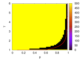
Figure 1: Final number of species $N_{s}$ on a random regular graph with $N=500$ nodes and $k=100$ (averaged over 200 realizations), as a function of the two parameters $p$ and $\gamma$. The yellow area corresponds to $500$ surviving species, while black area indicates only one surviving species. The red line marks the edge of stability for $S_{3}$ in the mean-field approximation.

The red line drawn in Fig. (1) is the numerical solution of Eq. (5) for different values of $(p,\gamma)$ and for $\varepsilon\rightarrow 0$ on a regular network with $N=500$ nodes. The state $S_{3}$ with $N$ surviving species is unstable for values of $(p,\gamma)$ below the red line, while it is stable for $(p,\gamma)$ above the red line. To check the validity of the mean–field approximation, we simulated the dynamics of Eq. (2) over a regular random graph with $N=500$ nodes, and a large average degree $k=100$, for different values of $(p,\gamma)$, initialising the system in state $S_{3}$. In Fig. (1) we plot as a colour map the number of species surviving at equilibrium for different values of $p$ and $\gamma$. Yellow regions correspond to $500$ surviving species, while black regions correspond to only one surviving species. Notice that the agreement with the theory is very good: the yellow area approximately coincides with the region where $S_{3}$ is stable, while the black zone corresponds to the region where $S_{3}$ is unstable. Notice also that the transition is very sharp and well defined in the $(p,\gamma)$ plane, meaning that the system suddenly moves from a state where $N_{s}=N$ to a state where $N_{s}=1$.

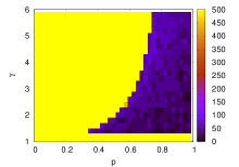
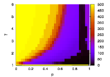
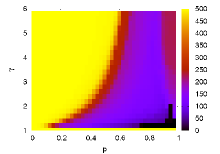
Figure 2: Number of species $N_{s}$ on the graph at equilibrium as a function of the two parameters $p$ and $\gamma$. Three classes of graphs with $N=500$ nodes and $\langle k\rangle=6$ were considered: a) regular ring lattice, b) Erdös–Renyi random graph, c) scale–free graph.

To explore the dependence of the dynamics on the degree distribution of the network, we have simulated Eq. (2) with initial state $S_{3}$ over three different networks, namely regular lattices (RL) with periodic boundary conditions, Erdös–Renyi (ER) random graphs, and scale–free (SF) graphs with degree distribution $P(K)\sim k^{-3}$ rev1 ; rev2 ; rev3 . All the graphs have been created with the same number of nodes ($N=500$) and the same number of links ($\langle k\rangle\simeq 6$). The phase diagrams in Fig. (2) show the number of species $N_{s}$ remaining at equilibrium on the three classes of graphs as a function of the two parameters $p$ and $\gamma$. We observed that a stationary value of $N_{s}$ is reached on these graphs after no more than $200$ iterations of Eq. (2), and we have checked that this value does not change for at least $20000$ iterations. Diagrams for ER and SF graphs are obtained as an average over 200 realizations, even if the fluctuations from one realization to another are very small. We notice that both $p$ and $\gamma$ play an important role on the final number of species remaining at equilibrium. For small $p$ and large $\gamma$ all the species survive, with each species remaining in its starting node. In fact, when $p$ is close to $0$, only a small amount of individuals leave their starting nodes and die almost immediately after they arrive at neighbouring nodes due to selection. This corresponds to the large yellow area ($N_{s}=500$) present in all the phase diagrams reported in Fig. (2). As the diffusion probability $p$ increases, a stronger selection (larger value of $\gamma$) is needed to prevent the invasion and let all the $N_{s}=500$ species survive. Despite some similarities for small $p$ and large $\gamma$, the three graphs exhibit different behaviour when diffusion and selection are such that some species can invade neighbouring nodes, and some other species eventually disappear. According to the values of $p$ and $\gamma$, the combination of diffusion and competition determines stationary solutions with different number $N_{s}$ of surviving species, also with a few remaining species, or even just one, as in the black regions. The differences between the three graphs are evident from the various sizes and shapes of the coloured regions. In both ER and scale-free graphs we have cases where only one species survives (black regions in Fig. (2) and in Fig. (2)) and invades the whole network. However, the black region is much larger in the phase diagram of the ER random graphs than in that of the scale-free graphs, where a single species overcomes all the others only when $p\sim 0.95$ and $\gamma\sim 1.2$. The differences between the phase diagrams of ER and SF graphs are due to the different degree distribution in the two graphs. In fact, the diffusion process naturally favours species starting at poorly connected nodes, since the average number of individuals of such species that will move to first neighbours is higher than the average amount of individuals coming from highly connected nodes. Hence, species starting at poorly–connected nodes have a higher probability to survive and to invade neighbours. In the ER graph, these are the few species that survive and invade the graph for $(p,\gamma)$ in the bottom–right part of the diagram (purple and black colour), with the competition process involving species starting at nodes with increasingly large degree, as $p$ decreases. The same considerations, based on neighbourhood invasion by species starting at poorly–connected nodes, hold for scale-free graphs as well, with the main difference that in a power–law degree distribution the majority of nodes are poorly–connected, while just a few hubs have a lot of links. Consequently, species starting at hubs will disappear soon, while a large number of species tends to survive for a wide range of $p$ and $\gamma$. This explains why the black region for SF graphs is much smaller than for ER graphs, and why at any given point $(p,\gamma)$ of the phase diagram, the number of species $N_{s}$ on an ER random graph is always equal or lower than the number of species on a scale-free graph. The diagram for a regular lattice reported in Fig. (2) is very similar to that shown in Fig. (1). These results confirm that the degree distribution of the network plays an important role in the extinction and survival of species. We have also investigated how the dynamics of the system depends on other structural properties of the network, namely the number of nodes, the average node degree, the clustering coefficient, degree–degree correlations and the presence of communities. In the following, we use an alternative method to display the information contained in the phase diagrams. Namely, we plot the cumulative distribution of the percentage of surviving species at equilibrium, over all the couples of parameters $(p,\gamma)$ in the phase diagram. This is useful to compare the phase diagrams corresponding to different networks.

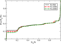
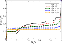
Figure 3: Cumulative distribution of surviving species in ER graphs for $0\leq p<1$ and $1<\gamma\leq 6$ (averaged over $200$ realizations). Panel (a) $\langle k\rangle=8$ and $N=500$, $N=1000$ and $N=2000$ nodes. Panel (b) $N=1000$ and different values of $\langle k\rangle$.

In Fig. (3) we report the cumulative distribution of the percentage of surviving species over $(p,\gamma)$ for three ER random graphs, having average degree $\langle k\rangle=8$ and size $N=500$, $N=1000$ and $N=2000$, respectively. For the ER random graph with $N=500$ nodes more than $22\%$ of the $(p,\gamma)$ values cause the invasion of the network by one species, and $N_{s}/N=1$ for more than $45\%$ of the $(p,\gamma)$ values. The percentage of pairs $(p,\gamma)$ which allow invasion by only one species decreases to $20\%$ and to $18\%$, respectively for $N=1000$ and $N=2000$, while there is no appreciable difference among the three curves for $N_{s}/N>0.4$. Therefore, for ER random graphs an increase in the network size producees a slight decrease of the area of the phase diagram for which we observe invasion by only one species. In Fig. (3) we compare ER random graphs with $N=1000$ nodes and different values of $\langle k\rangle$, namely $6,8,10,15,20$. As the average degree increases, the shape of the distribution tends to that of a homogenous network. In particular, for $\langle k\rangle=20$, the phase diagram is similar to a stepwise function: only one species survives for $25\%$ of the $(p,\gamma)$ pairs, while all the $N_{s}=1000$ initial species survive for more than $60\%$ of the possible $(p,\gamma)$ values.

While ER random graphs are characterised by the size of the network and by the average degree, networks from the real world usually show also non-trivial degree–degree correlations and a relatively high number of triangles. In Fig. (4) we report the cumulative distribution of surviving species at equilibrium for the US Airport network airports . This network has $N=500$ nodes, representing airports, $2980$ links, indicating flight connections, a degree distribution with a power–law tail with an exponent $\sim-1$, a clustering coefficient $C=0.62$ and disassortative degree–degree correlations. In the same figure we report the cumulative distribution of surviving species for a random graph having the same degree sequence of the US Airports network. The randomisation washes out all correlations, so that this network has $C=0.09$ and no degree–degree correlations. Notice that the US Airports network allows the survival of a higher percentage of species than its random counterpart. More than $85\%$ of $(p,\gamma)$ values guarantee the survival of more than $50\%$ of the species, and for more than $95\%$ of $(p,\gamma)$ values we observe survival of at least $40\%$ of the species. Conversely, in the random graph only $50\%$ of the species survive for $60\%$ of $(p,\gamma)$ values. This suggests that even if two networks have exactly the same degree distribution, the existence of clustering or degree–degree correlations favours the survival of a larger number of species.

We have also found that the presence of modules and communities can affect the dynamics of the system. In Fig. (4) we show the cumulative distribution of the percentage of surviving species for two standard benchmark networks having a predefined community structure (the Girvan–Newman’s benchmark (GN) newman_benchmark and the Lancichinetti–Fortunato–Radicchi’s benchmark (LFR) fortunato_benchmark ) and for the corresponding random graphs without any community structure. All the networks have $N=1000$ nodes. The GN benchmark is a regular network with $k=12$, while the LFR benchmark is a scale–free network with $P(k)\sim k^{-2}$ and $\langle k\rangle=6$. The two benchmark networks have $4$ communities of $250$ nodes each: on average, $90\%$ of the links of each node are inside its community and the remaining $10\%$ of links point to nodes outside the community. The distribution of surviving species in the LFR benchmark is very similar to that of a random scale–free graph: at least $50\%$ of the species survive for $90\%$ of $(p,\gamma)$ values and more than $70\%$ of the species survive for more than $45\%$ of $(p,\gamma)$ values. Conversely, the GN benchmark has a slightly different behaviour compared to the corresponding regular random graph. In the regular random graph only $1$ species eventually invades the network for $22\%$ of possible $(p,\gamma)$ values, while all $N_{s}$ species survive for $65\%$ of $(p,\gamma)$ pairs. For the GN benchmark, instead, more than $20\%$ of $(p,\gamma)$ pairs guarantee the survival of exactly $4$ species. We have checked that in this case each of the four surviving species is confined into one of the four communities, and that each node of a given community contains individuals of only one species. These results indicate that the existence of communities in the underlying network can affect the evolution of the system, especially in graphs with homogeneous degree distributions.

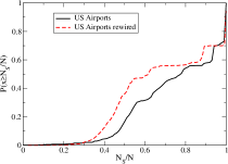
Figure 4: Panel (a): cumulative distribution of surviving species for the US Airports network and a random network with the same degree distribution. Panel (b): cumulative distribution of surviving species for the GN benchmark, the LFR benchmark, a random regular graph and a scale–free random graph. The two benchmark networks have $4$ communities of $250$ nodes each.

Summing up, we have found that network structure can strongly affect the dynamics of simple diffusion–competition processes. A central role in determining the strength of segregation and the number of surviving species at the equilibrium is played by the degree distribution. A network with heterogeneous degree distribution guarantees, for a wider ranges of diffusion and selection parameters, the survival of a higher number of species compared to the case of a homogeneous network. In particular, degree heterogeneity helps to avoid the invasion of the network by only one species. We have also investigated the effect of other structural properties, such as the size of the network, the average degree, the existence of degree–degree correlations and community structures. In conclusion, the results confirm that the actual structure of the network has to be taken seriously into account for the study of competitive processes on complex topologies, since small differences in the network structure can produce large differences in the observed dynamics. Our simple model sheds light on the role of the environment in diffusion–competition dynamics, and might find useful to explore how cultures, languages, biotypes and competing populations in general may survive or get extinct according to the structure of the network they live in.

References

- (1) Albert R., Barabási A.-L., Rev. Mod. Phys. 74, 47 (2002).
- (2) Newman M.E.J., SIAM Review 45, 67 (2003).
- (3) Boccaletti S. et al., Phys. Rep. 424, 175 (2006).
- (4) Pastor-Satorras R., Vespignani A., Phys. Rev. Lett. 86, 3200 (2001).
- (5) Noh J.D., Rieger H.,Phys. Rev. Lett. 92, 118701 (2004).
- (6) Gómez-Gardeñes J., Latora V., Phys. Rev. E 78, 065102(R) (2008).
- (7) Arenas A. et al., Phys. Rep. 469, 93 (2008).
- (8) Moreno Y., Gomez J. B., Pacheco A. F., Physica A 274, 400 (1999).
- (9) Jensen H.J., “Self–Organized Criticality”, Cambr. Univ. Pr. (1998).
- (10) Jensen H. J., Proc. Roy. Soc. A. 464, 2207 (2008).
- (11) Anderson P. E., Jensen H. J., J. Theor. Biol. 232, 551 (2005).
- (12) Schelling T. C., J. of Math. Soc. 1, 143 (1971).
- (13) Axelrod R., J. Conflict Resolution 41, 203 (1997).
- (14) Castellano C., Fortunato S., Loreto V., Rev. Mod. Phys. 81, 591 (2009).
- (15) Hofbauer J., Sigmund K., “Evolutionary Games and Population Dynamics”, Cambr. Univ. Pr. (1998).
- (16) Nowak M. A., “Evolutionary Dynamics: Exploring the Equations of Life”, Harv. Univ. Pr. (2006).
- (17) Santos F. C., Pacheco J. M., Phys. Rev. Lett. 95, 098104 (2005).
- (18) Gómez-Gardeñes J. et al., Phys. Rev. Lett. 98, 108103 (2007).
- (19) Tang J. et al., Phys. Rev. E 81, 055101(R) (2010).
- (20) Helbing D., Yu W., Proc. Natl. Acad. Sci. U.S.A. 106, 3680 (2009).
- (21) Meloni S. et al., Phys. Rev. E 79, 067101 (2009).
- (22) Guimerà R. et al. Proc. Natl. Acad. Sci. U.S.A. 102, 7794 (2005).
- (23) Eubank S. et al., Nature 429, 180 (2004).
- (24) Colizza V., Pastor-Satorras R., Vespignani A., Nat. Phys. 3, 276 (2007).
- (25) Bianconi G., Phys. Lett. A 303, 166 (2002).
- (26) Barrat A. et al., Proc. Natl. Acad. Sci. U.S.A. 101, 3747 (2004).
- (27) Girvan M., Newman M.E.J., Proc. Natl. Acad. Sci. U.S.A. 99, 7821 (2002).
- (28) Lancichinetti A., Fortunato S., Radicchi F., Phys.Rev. E 78, 046110 (2008).