The Lick-Carnegie Exoplanet Survey: A Uranus-mass Fourth Planet for GJ 876 in an Extrasolar Laplace Configuration

Abstract

Continued radial velocity monitoring of the nearby M4V red dwarf star GJ 876 with Keck/HIRES has revealed the presence of a Uranus-mass fourth planetary companion in the system. The new planet has a mean period of $P_{e}=126.6$ days (over the 12.6-year baseline of the radial velocity observations), and a minimum mass of $m_{e}\sin{i_{e}}=12.9\pm 1.7\,M_{\oplus}$. The detection of the new planet has been enabled by significant improvements to our radial velocity data set for GJ 876. The data have been augmented by 36 new high-precision measurements taken over the past five years. In addition, the precision of all of the Doppler measurements have been significantly improved by the incorporation of a high signal-to-noise template spectrum for GJ 876 into the analysis pipeline. Implementation of the new template spectrum improves the internal RMS errors for the velocity measurements taken during 1998-2005 from 4.1 m s^-1 to 2.5 m s^-1. Self-consistent, N-body fits to the radial velocity data set show that the four-planet system has an invariable plane with an inclination relative to the plane of the sky of $i=59.5^{\circ}$. The fit is not significantly improved by the introduction of a mutual inclination between the planets “b” and “c,” but the new data do confirm a non-zero eccentricity, $e_{d}=0.207\pm 0.055$ for the innermost planet, “d.” In our best-fit coplanar model, the mass of the new component is $m_{e}=14.6\pm 1.7\,M_{\oplus}$. Our best-fitting model places the new planet in a 3-body resonance with the previously known giant planets (which have mean periods of $P_{c}=30.4$ and $P_{b}=61.1$ days). The critical argument, $\varphi_{\rm Laplace}=\lambda_{c}-3\lambda_{b}+2\lambda_{e}$, for the Laplace resonance librates with an amplitude of $\Delta\varphi_{\rm Laplace}=40\pm 13^{\circ}$ about $\varphi_{\rm Laplace}=0^{\circ}$. Numerical integration indicates that the four-planet system is stable for at least a billion years (at least for the coplanar cases). This resonant configuration of three giant planets orbiting an M-dwarf primary differs from the well-known Laplace configuration of the three inner Galilean satellites of Jupiter, which are executing very small librations about $\varphi_{\rm Laplace}=180^{\circ}$, and which never experience triple conjunctions. The GJ 876 system, by contrast, comes close to a triple conjunction between the outer three planets once per every orbit of the outer planet, “e.”

1 Introduction

The planetary system orbiting the nearby M4V star GJ 876 (HIP 113020) has proven to be perhaps the most remarkable entry in the emerging galactic planetary census. This otherwise unassuming red dwarf has produced the first example of a giant planet orbiting a low-mass star, the first instance of a mean-motion resonance among planets, the first clear-cut astrometric detection of an extrasolar planet, and one of the first examples of a planet in the hitherto unknown mass regime between Earth and Uranus.

The radial velocity (RV) variations of GJ 876 have been monitored by us, the Lick-Carnegie Exoplanet Survey team (LCES), at the Keck I telescope using the High Resolution Echelle Spectrograph (HIRES) for 12.6 years. Bean & Seifahrt (2009) and Rivera et al. (2005) (R05 henceforth) give detailed discussions of the discoveries and some of the studies made for this system. Here, we summarize some of that history.

Marcy et al. (1998) and Delfosse et al. (1998) announced the first companion, “b.” They found that it has an orbital period ($P_{b}$) of $\sim 61$ days and a minimum mass ($m_{b}\sin{i_{b}}$) of $\sim 2.1\,M_{\rm Jup}$ and that it produced a reflex barycentric velocity variation of its host star of amplitude $K_{b}\sim 240$ m s^-1. After 2.5 more years of additional Doppler monitoring, Marcy et al. (2001) announced the discovery of a second giant planet in the system. This second companion, “c,” has an orbital period, $P_{c}\sim 30$ days, $m_{c}\sin{i_{c}}\sim 0.56\,M_{\rm Jup}$, and $K_{c}\sim 81$ m s^-1, and upon discovery of the second planet, the parameters of the first planet were tangibly revised. Marcy et al. (2001) modeled the two-planet system with non-interacting Keplerian orbits, and noted both that there was room for improvement in the quality of the fit and that the system’s stability depended on the initial positions of the planets.

To a degree that has not yet been observed for any other planetary system, the mutual perturbations between the planets are dynamically significant over observable time scales. This fortuitous situation arises because the minimum masses are relatively large compared to the star’s mass, because the planetary periods are near the 2:1 commensurability, and because their orbits are confined to a small region around the star.

Laughlin & Chambers (2001) and Rivera & Lissauer (2001) independently developed self-consistent “Newtonian” fitting schemes which incorporate the mutual perturbations among the planets in fitting the RV data. The inclusion of planet-planet interactions resulted in a substantially improved fit to the RV data, and suggested that the coplanar inclination of the b-c pair lies near $i=50^{\circ}$. These papers were followed by an article by Nauenberg (2002) who described a similar dynamical fitting method, but, in contrast, found a system inclination near $i=90^{\circ}$.

Soon after the announcement of planet “c,” Benedict et al. (2002) used the Fine Guidance Sensor on the Hubble Space Telescope to detect the astrometric wobble induced by planet “b,” which constituted the first unambiguous astrometric detection of an extrasolar planet. Their analysis suggested that the orbital inclination of planet “b” is close to edge-on ($i_{b}=84^{\circ}\pm 6^{\circ}$), a result that agreed with the model by Nauenberg (2002), but which was in conflict with the results of Laughlin & Chambers (2001) and Rivera & Lissauer (2001).

R05 analyzed an updated RV data set that included new Doppler velocities obtained at Keck between 2001-2005. By adopting self-consistent fits, they were able to announce the discovery of a third companion, “d,” with period $P_{d}\sim 1.94$ days, $m_{d}\sin{i_{d}}\sim 5.9\,M_{\oplus}$, and $K_{d}\sim 6.5$ m s^-1. Using only the RV data, they were able to constrain the inclination of the system (assuming all three planets are coplanar) relative to the plane of the sky to $50\pm 3^{\circ}$. For this inclination, the true mass of the third companion is $\sim 7.5\,M_{\oplus}$.

Bean & Seifahrt (2009) performed self-consistent fitting of both the Keck RV data from R05 and the astrometry from Benedict et al. (2002). They found the that the joint data set supports a system inclination $i=48.9^{+1.8^{\circ}}_{-1.6^{\circ}}$, which is in agreement with the $i=50\pm 3^{\circ}$ value published by R05. Bean & Seifahrt’s analysis (see, e.g. their Figure 1) indicates that the best-fit $\chi_{\nu}^{2}$ is not significantly affected by the inclusion of the astrometric data, and that the astrometric detection of “b” by Benedict et al. (2002) is not in conflict with the significantly inclined system configuration. Bean & Seifahrt’s work also resulted in the first determination of a mutual inclination between the orbits of two planets in an extrasolar planetary system. By allowing the inclinations, $i_{b}$, and $i_{c}$, and the nodes, $\Omega_{b}$, and $\Omega_{c}$ to float as free parameters in their three-planet dynamical fit, they derived a mutual inclination, $\cos{\Phi_{bc}}=\cos{i_{b}}\cos{i_{c}}+\sin{i_{b}}\sin{i_{c}}\cos{(\Omega_{c}-\Omega_{b})}$, of $\Phi_{bc}=5.0^{+3.9^{\circ}}_{-2.3^{\circ}}$.

Correia et al. (2009) also performed self-consistent, mutually inclined fits using the RVs from R05 plus 52 additional high precision RV measurements taken with the HARPS spectrograph. They confirmed the presence of companion “d,” and further showed that it has a significant orbital eccentricity, $e_{d}=0.139\pm 0.032$. Correia et al. (2009) determined inclinations $i_{b}=48.93^{\circ}\pm 0.97^{\circ}$ and $i_{b}=48.07^{\circ}\pm 2.06^{\circ}$. Their orbital fit yields a mutual inclination $\Phi_{bc}=1.00^{\circ}$, consistent to within measurement uncertainty with a coplanar system configuration. We became aware of Correia et al. (2009) while preparing this article for publication. A. Correia (2009, personal communication) graciously shared the HARPS radial velocity data on which their paper is partly based. We have carried out a preliminary analysis that indicates that our new results are not in conflict with these HARPS data. The HARPS RVs do not add much to constrain the system’s dynamics because of poor phase coverage at the period of the forth planet to be discussed below. Throughout this article, however, our analysis and results are based on the Keck RVs alone.

In addition to R05, several other studies, such as West (1999), West (2001), Laughlin et al. (2005), and Shankland et al. (2006), have examined the possibility of transits occurring in this system. The star has also been included in surveys in which it was probed for nearby companions or a circumstellar dust disk. These include Leinert et al. (1997), Patience et al. (2002), Hinz et al. (2002), Trilling et al. (2000), Lestrade et al. (2006), Shankland et al. (2008), and Bryden et al. (2009). Luhman & Jayawardhana (2002) were able to use Keck AO to place limits on potential brown dwarfs in the system at separations of 1 – 10 AU. Seager & Deming (2009) used the Spitzer spacecraft to search for thermal emission from planet “d.” The star was also included in the Gemini Deep Planet Survey (Lafreniere et al., 2007). In addition to some of the work above, a variety of studies have examined the dynamics, and/or long-term stability of the system. Examples are Kinoshita & Nakai (2001), Gozdziewski & Maciejewski (2001) and Gozdziewski et al. (2002), Snellgrove et al. (2001), Ji et al. (2002), Jones et al. (2001), Zhou & Sun (2003), and Haghighipour et al. (2003). Beauge & Michtchenko (2003) present an analytic model which does a very good job at reproducing the dynamical evolution of the system. Murray et al. (2002), Lee & Peale (2002), Chiang et al. (2002), Thommes & Lissauer (2003), Beauge et al. (2003), Kley et al. (2004), Lee (2004), Kley et al. (2005), and Lee & Thommes (2009) examined scenarios of how the system may have come to be in its current dynamical configuration. Even interior structure models of GJ 876 d have been introduced (Valencia et al., 2007).

In this work, we present a detailed examination of our significantly augmented and improved HIRES RV data set from the Keck observatory. Our analysis indicates the presence of a fourth, Uranus-mass planet in the GJ 876 system. The new planet is in a Laplace resonance with the giant planets “b” and “c,” and the system marks the first example of a three-body resonance among extrasolar planets. We expect that the newly resolved presence of the fourth planet will provide additional constraints on the range of formation scenarios that could have given rise to the system, and will thus have a broad impact on current theories for planetary formation. The plan for this paper is as follows: In § 2, we describe the new velocities and the methods used to obtain them. In § 3, we present our latest two- & three-planet coplanar fits. In § 4, we thoroughly analyze the residuals of our best three-planet coplanar fits. In § 5, we discuss our four-planet fits. In § 6 we explore the possibility of constraining the libration amplitude of the critical angle for the Laplace resonance. In § 7 we explore the stability of additional planets in the system. Finally, in § 8, we finish with a summary and a discussion of our findings.

2 Radial Velocity Observations

The stellar characteristics of GJ 876 have been described previously in Marcy et al. (1998) and Laughlin et al. (2005). It has a Hipparcos distance of 4.69 pc (Perryman et al., 1997). Its luminosity is 0.0124 $L_{\odot}$. As in previous studies, we adopt a stellar mass of $0.32\,M_{\odot}$ and a radius of $0.3\,R_{\odot}$ based on the mass-luminosity relationship of Henry & McCarthy (1993). We do not incorporate uncertainties in the star’s mass ($0.32\,\pm\,0.03\,M_{\odot}$) into the uncertainties in planetary masses and semi-major axes quoted herein. The age of the star exceeds 1 Gyr (Marcy et al., 1998).

We searched for Doppler variability using repeated, high resolution spectra with resolving power $R\approx 70000$, obtained with Keck/HIRES (Vogt, et al., 1994). The Keck spectra span the wavelength range from 3700 – 8000 Å. An iodine absorption cell provides wavelength calibration and the instrumental profile from 5000 to 6200 Å (Marcy & Butler, 1992; Butler et al., 1996). Typical signal-to-noise ratios are 100 per pixel for GJ 876. At Keck we routinely obtain Doppler precision of better than 3 – 5 m s^-1 for V = 10 M dwarfs. Exposure times for GJ 876 and other V = 10 M dwarfs were typically 8 minutes. Over the past year, these typical exposure times have been raised to 10 minutes.

The internal uncertainties in the velocities are judged from the velocity agreement among the approximately 700 2-Å  chunks of the echelle spectrum, each chunk yielding an independent Doppler shift. The internal velocity uncertainty of a given measurement is the uncertainty in the mean of the $\sim 700$ velocities from one echelle spectrum.

We present results of N-body fits to the RV data taken at the W. M. Keck telescope from 1997 June to 2010 January. The 162 measured RVs are listed in Table 1. The median of the internal uncertainties is 2.0 m s^-1. Comparison of these velocities with those presented in Laughlin et al. (2005) and in R05 shows significant changes (typically 3 – 10 m s^-1) in the velocities at several observing epochs. R05 discuss the primary reasons for the improvements — a CCD upgrade and an improved data reduction pipeline. Additionally, many of the velocities presented here are the result of averaging multiple exposures over two-hour time bins. More importantly, the present RV data set is based on a new “super” template. For the new template, ten exposures, most of which were $<900$ sec, were obtained under very good observing conditions. In contrast, the template used to determine the RVs and uncertainties in R05 was based on only three 900-sec exposures taken under relatively poor observing conditions. As a result, the new template has brought the median internal uncertainty down to the current 2.0 m s^-1 from the value of 4.1 m s^-1 in R05. Additionally, the new template has resulted in significant changes in the old published RVs. Note that since the last observation listed in R05, 36 more high quality observations have been obtained for this system since 2004 December. Our LCES survey assigns high observing priority to GJ 876, given the potential for further characterizing the intricate dynamical configuration between the 30- and 61-day planets and because of the possibility of detecting additional planets in the system.

Table 1: Measured Velocities for GJ 876 (Keck)

BJD	RV	Unc.
(-2450000)	(m s-1)	(m s-1)
602.09311	329.19	1.79
603.10836	345.30	1.81
604.11807	335.99	1.92
605.11010	336.00	1.93
606.11129	313.94	1.88

Note. — Table 1 is presented in its entirety in the electronic edition of the Astrophysical Journal. A portion is shown here for guidance regarding its form and content.

3 Two- & Three-Planet Coplanar Fits

We used similar procedures to those described in R05 to produce updated two- and three-planet dynamical fits to the GJ 876 Doppler velocities. The epoch for all the fits in this work is JD 2450602.093. As in R05, we initially held the eccentricity of companion “d” ($e_{d}$) fixed. We find, however, that fitting for $e_{d}$ results in a significant improvement in all the fits which include companion “d.” We therefore allow $e_{d}$ to float in our final fits. Uncertainties in the tables listing our best-fit jacobi parameters are based on 1000 bootstrap realizations of the RV data set. We take the uncertainties to be the standard deviations of the fitted parameters to the 1000 trials. The fitting algorithm is a union of Levenberg-Marquardt (LM) minimization (§15.5 of Press et al. (1992)) and the Mercury integration package (Chambers, 1999).

Our dynamical fits can be integrated to determine the libration amplitudes of the critical arguments of the 2:1 MMR between “b” and “c,” and to monitor the linear secular coupling between the pericenter longitudes. For each fit, we integrated the system for 300,000 days ($\sim$821 years) with a timestep of 0.05 day. For all simulations in this work, we used the Hybrid symplectic algorithm in the Mercury integration package (Chambers, 1999) modified as in Lissauer & Rivera (2001) to include the partial first order post-Newtonian correction to the central star’s gravitational potential. The three relevant angles are $\varphi_{cb,c}=\lambda_{c}-2\lambda_{b}+\varpi_{c}$, $\varphi_{cb,b}=\lambda_{c}-2\lambda_{b}+\varpi_{b}$, and $\varphi_{cb}=\varphi_{cb,b}-\varphi_{cb,c}=\varpi_{b}-\varpi_{c}$. For each of these angles, we measure the amplitude as half the difference between the maximum and minimum values obtained during each $\sim$821-year simulation. As expected, we find that for both two- and three-planet fits to the real data set and for every bootstrapped data set, all three angles librate about 0^∘. We use the subscript “cb” to indicate the angles relating the longitudes of planets “c” and “b.” In § 5, we will use the subscripts “be” and “ce” to indicate the corresponding angles relating the longitudes of planets “b” and “e,” and “c” and “e,” respectively.

As in R05, we inclined the coplanar system to the line-of-sight. We set the inclination relative to the plane of the sky of all the companions to values from 90^∘ to 40^∘ in decrements of 1^∘. We hold all the longitudes of the ascending node fixed at 0^∘. We fit for all the remaining parameters. Finally, we examine $\chi_{\nu}^{2}$ as a function of the system’s inclination. Figure 1 shows the results.

The minimum in $\chi_{\nu}^{2}$ as a function of the system’s inclination is in the range 57 – 61^∘. We find that the location of the minimum has a small dependence on the number of companions in the system. For two planets, we find $i=57\pm 5.8^{\circ}$. For three planets, we find $i=59\pm 3.2^{\circ}$. For four planets, we find $i=61\pm 2.4^{\circ}$. (The results for four-planet fits are presented in § 5). The error estimates on the coplanar inclination are derived from 100 bootstrap trials of the RV data set. For each bootstrap RV set, we use the best-fit parameters to the real RVs at each inclination value as the initial guess. For each trial, we find the minimum in $\chi_{\nu}^{2}$ as a function of the system’s inclination. The uncertainties in the fitted inclination of the system are the standard deviations of the locations of the minimum in $\chi_{\nu}^{2}$. Our best three- and four-planet dynamical fits indicate a system with an invariable plane with an inclination relative to the plane of the sky of $\sim 59^{\circ}$, and we adopt this inclination as a starting point for studying the fitness of models with mutually inclined orbits.

Starting from the coplanar, $i=59^{\circ}$, two-planet fit, we examine the effect of a mutual inclination between companions “b” and “c.” We do this by fitting for the inclinations of “b” and “c” ($i_{b}$ and $i_{c}$) and the longitude of the ascending node of “c” ($\Omega_{c}$). Since the system is rotationally invariant about the line-of-sight, we leave the longitude of the ascending node of “b” ($\Omega_{b}$) fixed at 0^∘. We find $\chi_{\nu}^{2}=9.76$ (rms$=$5.704 m s^-1) for the coplanar fit, and $\chi_{\nu}^{2}=9.91$ (rms$=$5.706 m s^-1) for the mutually inclined fit. This “improvement” is not significant. As we show below, fitting for the mutual inclination of “b” and “c” in the case of four-planet configurations results in a similar “improvement” in $\chi_{\nu}^{2}$. For the two-planet mutually inclined model, the fitted masses and inclinations are $m_{c}=0.7211\,M_{\rm Jup}$, $m_{b}=2.3689\,M_{\rm Jup}$, $i_{c}=57.94^{\circ}$, and $i_{b}=55.29^{\circ}$, and $\Omega_{c}=0.82^{\circ}$. With the approximation that $\Omega_{c}\sim 0^{\circ}$, the invariable plane of this two-planet system has an inclination relative to the plane of the sky of $56^{\circ}$. The mutual inclination for this system is 2.7^∘.

For the three-planet model with $i=59^{\circ}$, our best coplanar fit has $\chi_{\nu}^{2}=3.93$ (rms$=$3.625 m s^-1), and the mutually inclined fit has $\chi_{\nu}^{2}=3.99$ (rms$=$3.620 m s^-1). For the mutually inclined fit, the invariable plane of the system has an inclination relative to the plane of the sky of $59.2^{\circ}$. For the mutually inclined fit, we force planet “d” to be in the invariable plane determined by “b” and “c.” The mutual inclination between “b” and “c” in this configuration is 0.7^∘. Since a mutual inclination does not significantly improve the three-planet fit, in Table 2 we show the best-fit parameters for our best coplanar three-planet fit.

At $i=59^{\circ}$, the angles $\varphi_{cb,c}$, $\varphi_{cb,b}$, and $\varphi_{cb}$ are all in libration for both the model fit (in Table 2) and for all of the bootstrap trials. For the fit in Table 2, these amplitudes are $\varphi_{cb,c}=4.5\pm 0.7^{\circ}$, $\varphi_{cb,b}=13.1\pm 3.2^{\circ}$, and $\varphi_{cb}=11.5\pm 3.7^{\circ}$. Note that the libration amplitudes for the three-planet fits presented in this section are smaller than for the three-planet fits presented in R05.

The critical angles show a complicated evolution for the coplanar three-planet fit with $i=59^{\circ}$. The first angle, $\varphi_{cb,c}$, has peaks at (listed with decreasing power) 1.58, 45.67, and 8.69 years. The second angle, $\varphi_{cb,b}$, has peaks at 8.69, 1.58, and 45.74 years. Finally, the third angle, $\varphi_{cb}$, has two peaks at 8.69 and 45.67 years. These periodicities are also present in the evolution of the eccentricities of the two outer planets. The eccentricities of all three planets show very regular secular evolution.

Figure 1: For GJ 876, $\chi_{\nu}^{2}$ as a function of the coplanar system’s inclination to the plane of the sky. The different types of points indicate how many planets are assumed to be in the system. Triangles are for two planets, squares are for three planets, and pentagons are for four planets. The eccentricity of “d” is allowed to float for all of the three- and four-planet fits used to make this figure. Note that the minimum is better constrained with the addition of each planet.

Table 2: Three-Planet coplanar fit for GJ 876 with $i=59^{\circ}$

Parameter	Planet d	Planet c	Planet b
$P$ (days)	$1.937781\pm 0.000024$	$30.0880\pm 0.0091$	$61.1139\pm 0.0084$
$m$	$6.78\pm 0.51\,M_{\oplus}$	$0.7175\pm 0.0042\,M_{\rm Jup}$	$2.2743\pm 0.0059\,M_{\rm Jup}$
$a$ (AU)	$0.02080665\pm 0.00000018$	$0.129590\pm 0.000026$	$0.208301\pm 0.000019$
$K$ (m s-1)	$6.60\pm 0.47$	$88.72\pm 0.52$	$213.86\pm 0.55$
$e$	$0.257\pm 0.070$	$0.25493\pm 0.00080$	$0.0292\pm 0.0015$
$\omega$ (∘)	$229\pm 28$	$48.67\pm 0.82$	$50.7\pm 4.5$
MA (∘)	$358\pm 29$	$295.0\pm 1.0$	$325.4\pm 4.6$
offset (m s-1)	$50.7\pm 0.4$
Fit Epoch (JD)	2450602.093
$\chi_{\nu}^{2}$	3.9280
RMS (m s-1)	3.6254
$\varphi_{cb,c}$	$4.5\pm 0.7^{\circ}$
$\varphi_{cb,b}$	$13.1\pm 3.2^{\circ}$
$\varphi_{cb}$	$11.5\pm 3.7^{\circ}$

4 Residuals of the Three-Planet Fit

We performed an error-weighted Lomb-Scargle periodogram (Gilliland & Baliunas, 1987) analysis on the residuals of the coplanar three-planet fits for both $i=90^{\circ}$ and $i=59^{\circ}$. Both periodograms show a significant peak at $\sim$125 days. Figure 2 shows the periodogram for the case $i=59^{\circ}$. The periodogram for the case $i=90^{\circ}$ looks very similar. For $i=90^{\circ}$, the peak raw power is 311.4. For $i=59^{\circ}$, the peak raw power is 310.2. Even if we allow for a mutual inclination between “b” and “c” and an overall trend as in Correia et al. (2009) (they actually subtract out a trend, due to the geometrical effect of the star’s proper motion, prior to fitting the RVs), we still see a strong signal near 125 days in the periodogram of the residuals. For both values of $i$, folding the three-planet residuals at the peak period shows a strong coherent sinusoidal signature. Figure 3 shows the folded residuals for the case $i=59^{\circ}$. Examination of all the inclined three-planet fits shows that the peak period in the residuals is at 125 days for all values of $i\geq 40^{\circ}$. For the 1000 fits used in determining the uncertainties in Table 2, the residuals of 941 of them have a peak period near 125 days, with 12 harboring a marginally higher alias peak with a period near 1.0 days. The 125-day periodicity has been adequately sampled at all phases only relatively recently.

We also examined subsets of the RV data where we took just the first $N$ observations, assumed $i=59^{\circ}$, and fit for the parameters of the three known planets. We took all values of $N$ from 98 to 162. We then examined the error-weighted Lomb-Scargle periodogram of the residuals for all values of $N$. All the periodograms have a peak period near 125 days. In Figure 3 we show the folded residuals for the first 98 observations as squares. Comparison between the folded residuals for the first 98 points and that for the full RV set again suggests that the 125-day periodicity has been sampled at all phases only recently. The observed power at 125 days has grown monotonically during the last decade, but the growth rate has been non-uniform. The power grows more quickly whenever we observe around the time when the fourth planet is near the phases in its orbit when its orbital velocity has a large component along the line-of-sight. The power grows less quickly whenever we observe the system when the orbital motion of the fourth planet is mostly perpendicular to the line-of-sight. We are constrained to observe near the time of the full Moon, which impedes the efficiency of obtaining uniform phase coverage for periodicities near 120 days. As a consequence, there were several stretches where we consistently observed near the phases when the fourth planet’s orbital motion was primarily perpendicular to the line-of-sight. This circumstance is one of the reasons why so many observations over 12 years were required prior to reliably detecting the fourth periodicity in this system.

As an additional check on the reality of the 125-day signal, we ran a Monte Carlo analysis. We take the coplanar three-planet model at $i=59^{\circ}$ and integrate forward to generate a synthetic RV curve. We then generate a set of 1000 synthetic data sets by repeatedly sampling the synthetic RV curve at the times of the Keck observations and adding Gaussian noise perturbations of amplitude equal to the rms of the fit in Table 2. Then, for each RV set, we fit for the three planets and examine the periodogram of the residuals. In not one instance did the power near 125 days exceed the value observed for the real data. Additionally, the peak period is “near” 125 days in only one of the 1000 cases. Thus, the false alarm probability (FAP) is $<0.001$.

An alternative to the fourth planet hypothesis is that the 125-day periodicity is due to rotation of the star itself. The rotation period of GJ 876 is at least $\sim 40$ days, based on its narrow spectral lines and its low chromospheric emission at Ca II H&K (Delfosse et al., 1998). R05 presented photometric evidence of a rotation period of $\sim$97 days. Our measurements of the Mt. Wilson S activity index also confirms this rotation period. Thus, rotational modulation of surface features cannot explain the 125-day period in the velocities. The periodogram of our measured Mt. Wilson S activity index after subtracting out a 14-year spot cycle has a peak period near 88 days.

Figure 2: Error-weighted periodogram of the residuals of the three-planet coplanar fit, with $i=59^{\circ}$, to the RV data of GJ 876.

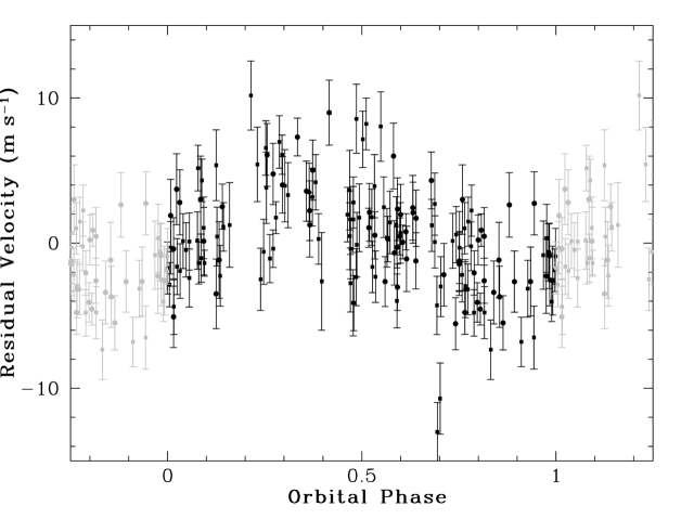
Figure 3: Residuals of the three-planet coplanar fit, with $i=59^{\circ}$, to the RV data of GJ 876. The residuals have been folded at the period of the tallest peak in the periodogram of the residuals. The first 98 observations are shown as squares.

5 Four-Planet Fits

The 125-day periodicity in the residuals to our best coplanar three-planet fit motivates exploration of the possibility that a fourth companion exists in the system. For the past several years, as we accumulated new RV measurements, we monitored the quality of dynamical fits containing a fourth planet with $P\sim 125$ days. From late 2005 through 2008, these fits preferred a fourth planet with $e_{e}>0.2$, and produced system configurations which, when integrated, were dynamically unstable. Only recently, have the four-planet fits resulted in systems which are stable on time scales exceeding a few hundred million years (at least for coplanar configurations). A fourth planet, with a mass similar to Uranus, and on a stable, low-eccentricity orbit, has now definitively emerged from the data.

A primary reason why the latest fits result in a stable system is that we have only recently gathered enough observations to sample all phases of the 125-day periodicity. Figure 3 shows that most of the (small) phase gaps have now been filled in. Additionally, near the points with larger residuals, we also have additional observations with smaller residuals. As a result, the LM routine no longer prefers a fourth planet with period $\sim$125 days with a relatively large eccentricity. Another reason why it has been difficult to find stable four-planet fits with the fourth planet at 125 days is that the region around the outer 2:1 MMR with companion “b” contains the boundary between stable and unstable orbits for the two-planet system consisting of only “c” and “b” (Rivera & Haghighipour, 2007).

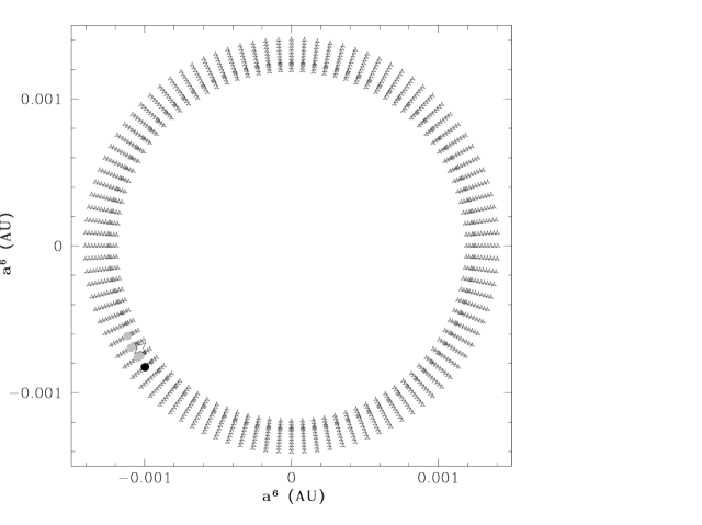
Figure 4: Stability of massless test particles placed at equally spaced initial longitudes on circular orbits with periods of 120 – 125 days in the plane of the system based on the fit from Table 2. For clarity, we show the astrocentric semi-major axes raised to the sixth power. Unstable locations are indicated with dark grey open symbols. The single “stable” location is indicated with a black filled-in symbol. The fitted initial location of the fourth planet from the fit in Table 3 is marked as an open star. Stable locations under the assumption $e_{d}=0$ are indicated with light grey filled-in symbols.

To highlight the generally tenuous stability of planets with periods near 125 days, we performed simulations based on the fit in Table 2 in which we added 1200 (massless) test particles on circular orbits in the plane of the system with periods in the range 120 – 125 days every 0.5 days plus at the fitted period for “e.” At each period we placed 100 test particles equally spaced in initial longitude. In agreement with Rivera & Haghighipour (2007), nearly all are unstable on time scales $<10^{6}$ years. Only one particle survived more than $10^{6}$ years; however, it was also lost after 7.4 Myr. It started with a period of 122.5 days (astrocentric) at a mean anomaly of 219.6^∘. For this long-term survivor the critical angle, $\varphi_{\rm Laplace}=\lambda_{c}-3\lambda_{b}+2\lambda_{e}$, librates around 0^∘ with an amplitude of $\Delta\varphi_{\rm Laplace}=22^{\circ}$ for the entire time that the particle is stable. The chaotic nature of the particle’s orbit becomes apparent when the libration amplitude of the Laplace angle suddenly becomes unconstrained during the last few thousand years of its evolution. In Figure 4 we show the stability of the test particles as a function of initial semi-major axis and longitude. For clarity, we show the astrocentric semi-major axes raised to the sixth power. Unstable initial locations are indicated with open dark grey symbols. The single “stable” initial location, where a test particle survived 7.4 Myr, is indicated with a filled-in black symbol. With an open star, we also mark the approximate fitted location for the fourth planet from the coplanar four-planet fit with $i=59^{\circ}$ (for simplicity, we assume zero eccentricity for the fourth planet — the astrocentric eccentricity is actually 0.0448). We also find that if we assign a mass of a few Earth masses to these “test particles,” they tend to survive for longer times. The results strongly suggest that a resonant mechanism is required for an object in this region to be stable.

Additionally, we find that the orbital parameters of the innermost planet, “d,” can influence the stability and chaotic nature of test particles placed in the region near 125 days. Assuming a circular orbit for “d” results in an island of stability near the fitted location of planet “e.” Instead of only a single particle which survives for 7.4 Myr, six particles survive for at least 10 Myr in this region if $e_{d}$ is assumed to be zero. As for the long-lived particle for the case with $e_{d}>0$, all the “stable” particles are in the Laplace resonance. The six stable particles under the assumption $e_{d}=0$ are shown as filled-in light grey symbols in Figure 4. We also used the Lyapunov estimator in the SWIFT integration package (Levison & Duncan, 1994) to analyze the chaotic nature of test particle orbits with periods near 125 days. We find that the most stable particles in this region have Lyaponov times in the range 10³ to 10⁴ years.

Following procedures similar to the ones used for the two- and three-planet fits, we worked up four four-planet fits. The best-fit coplanar inclination ($i=59^{\circ}$) with $e_{d}=0$ has $\chi_{\nu}^{2}=2.8738$ (rms=3.0655 m s^-1). Working from this fit, holding $e_{d}$ fixed, but fitting for a mutual inclination between “b” and “c” gives $\chi_{\nu}^{2}=2.8322$ (rms=3.0219 m s^-1). If instead we fit for $e_{d}$ and assume a coplanar system, the best-fit inclination is at $i=61^{\circ}$ and $\chi_{\nu}^{2}=2.5991$ (rms=2.9492 m s^-1). Finally, fitting for $e_{d}$ and a mutual inclination between “b” and “c” results in $\chi_{\nu}^{2}=2.6098$ (rms=2.9303 m s^-1). Since fitting for $e_{d}$ and the mutual inclination between “b” and “c” results in a significant improvement in $\chi_{\nu}^{2}$, we take this last model to represent our current best fit to the present Keck RV data set. However, simulating this model as well as other mutually inclined models with similar values of $\chi_{\nu}^{2}$ shows that the resulting systems are unstable on time scales of $\lesssim 1$ Myr. Also, with $e_{d}$ allowed to float, the “improvement” in $\chi_{\nu}^{2}$ between the coplanar and mutually inclined models is not significant. The F-Test probability that these two fits are statistically the same is 0.88. Thus, Table 3 shows the best-fit parameters for the coplanar four-planet fit with $i=59^{\circ}$, our preferred inclination for the system. The resulting system is stable for at least 300 Myr, and other coplanar fits with similar values of $\chi_{\nu}^{2}$ result in systems which are stable for hundreds of millions of years up to at least 1 Gyr.

For completeness, we note that for our best-fit mutually inclined system, the invariable plane of the system is inclined $59.5^{\circ}$ to the plane of the sky, and the mutual inclination between “b” and “c” is 3.7^∘. Fitting for the inclinations of planets “d” and “e” does not improve $\chi_{\nu}^{2}$ significantly. This result for the inclination of “d” is in agreement with the similar result by Correia et al. (2009). The F-Test probability for our best four-planet (mutually inclined) fit versus the three-planet coplanar fit with $i=59^{\circ}$ and with a fitted $e_{d}$ is 0.0066. This small probability indicates that the four-planet model is significantly different from the three-planet model. It should be noted that for the coplanar case with $i=59^{\circ}$ the fitted longitude of planet “e” is near the location of the long-lived particle discussed above.

The inclination of planet “e” does have a significant effect on the stability of the system based on our best mutually inclined fit. It also influences the libration amplitudes of the critical angles to be discussed below. The orbit of planet “e” must have an inclination and node such that the precession rates of both the nodes and longitudes of periastron of the outer three planets result in a relatively small libration amplitude for the critical angle of the Laplace resonance, $\varphi_{\rm Laplace}=\lambda_{c}-3\lambda_{b}+2\lambda_{e}$. In other words, systems with a small forced inclination for “e” should be more stable than systems with a large forced inclination – through experimentation we find this to be true. The coplanar four-planet fits are generally more stable than the mutually inclined versions since a small libration amplitude for $\varphi_{\rm Laplace}$ depends only on the precession rates of the longitudes of periastron of the outer three planets and not on the rates of precession of their nodes. For the mutually inclined four-planet fit, we performed a brief search of the parameter space spanned by $i_{e}$ and $\Omega_{e}$ as well as $i_{d}$ and $\Omega_{d}$. Experimentation shows that all four of these can influence the stability (and evolution) of this chaotic system. Also, the libration amplitudes of all the librating critical angles are smaller than if we simply place “e” and “d” in the invariable plane determined by “b” and “c.” Since we only explored a small region of the parameter space, and since we found several equally good fits to the RV data with various values for the forced inclination of “e,” other, more stable systems with smaller forced inclinations are likely to exist. One emerging pattern from the search of the parameter space is that smaller forced inclinations, smaller libration amplitudes, and more stable systems occur more likely for models in which the orbital plane of “e” is more closely aligned with that of “b.” This pattern is also in rough agreement with the finding that coplanar systems are generally more stable than mutually inclined ones.

As for the two- and three-planet fits, the critical angles involving “c” and “b” librate about $0^{\circ}$ for all our four-planet fits as well as for all 1000 bootstrap fits used in determining the uncertainties in Table 3. However, their amplitudes are generally larger because of the perturbing influence of the fourth planet.

Since the $\sim$125-day period is near the 2:1 MMR with planet “b,” the 4:1 MMR with planet “c,” and the Laplace resonance with both “b” and “c,” it is informative to examine all the relevant critical angles associated with these resonances as well as those associated with the resonances involving only “b” and “c.” For the 2:1 MMR and the linear secular coupling between “b” and “e,” the relevant angles are $\varphi_{be,b}=\lambda_{b}-2\lambda_{e}+\varpi_{b}$, $\varphi_{be,e}=\lambda_{b}-2\lambda_{e}+\varpi_{e}$, and $\varphi_{be}=\varphi_{be,e}-\varphi_{be,b}=\varpi_{e}-\varpi_{b}$. For the 4:1 MMR between “c” and “e,” there are 4 relevant angles: $\varphi_{ce0}=\lambda_{c}-4\lambda_{e}+3\varpi_{c}$, $\varphi_{ce1}=\lambda_{c}-4\lambda_{e}+2\varpi_{c}+\varpi_{e}$, $\varphi_{ce2}=\lambda_{c}-4\lambda_{e}+\varpi_{c}+2\varpi_{e}$, and $\varphi_{ce3}=\lambda_{c}-4\lambda_{e}+3\varpi_{e}$. The subscripts above correspond to the multiplier in front of $\varpi_{e}$. There is also, the critical angle involving just the longitudes of periastron of “c” and “e”: $\varphi_{ce}=\varpi_{e}-\varpi_{c}$. Finally, the critical angle for the Laplace resonance is $\varphi_{\rm Laplace}=\lambda_{c}-3\lambda_{b}+2\lambda_{e}$. Table 4 lists the libration amplitudes of all these critical angles for the fit in Table 3. A “C” in the amplitude column indicates that the angle circulates (at least once) during the $\sim$821-year simulation. The time evolution of the planetary eccentricities and the Laplace angle for the fit in Table 3 are shown in Figures 5 and 6, respectively. The secular evolution of the eccentricities of planets “b,” “c,” and “d” is apparently slightly less regular as a result of the addition of planet “e,” of which the eccentricity evolution is more chaotic than that of the other three planets. Additionally, the evolution of all the librating angles in stable four-planet fits appears chaotic; however, the resulting systems are stable for at least several hundreds of millions of years.

The addition of the low-mass planet “e” to the system model has only a modest effect on the dynamical characterization of the orbits of “b” and “c.” $\Delta\varphi_{cb,c}$ is increased from $4.5^{\circ}\pm 0.7^{\circ}$ to $5.74^{\circ}\pm 0.85^{\circ}$, and $\Delta\varphi_{cb}$ increases from $11.5^{\circ}\pm 3.7^{\circ}$ to $22.5^{\circ}\pm 4.8^{\circ}$. (Additionally, their evolution appears less regular with the addition of “e.”) In addition, the 4:1 argument, $\varphi_{ce0}$, is observed to librate with $\Delta\varphi_{ce0}=83^{\circ}\pm 25^{\circ}$, and the 2:1 argument $\varphi_{be,b}$ librates with $\Delta\varphi_{be,b}=36^{\circ}\pm 13^{\circ}$. Most significantly, the system also participates in the three-body resonance, with $\Delta\varphi_{\rm Laplace}=40^{\circ}\pm 13^{\circ}$.

Libration of $\varphi_{\rm Laplace}$ is required for stability. Long-term simulations based on bootstrap fits associated with four-planet coplanar fits indicate that systems for which $\varphi_{\rm Laplace}\gtrsim 140^{\circ}$ are unstable on time scales $<2$ Myr. Other systems with large libration amplitudes for $\varphi_{\rm Laplace}$, $141.4^{\circ}$, $129.1^{\circ}$, and $119.4^{\circ}$, are stable for only 25.9 Myr, 33.6 Myr, and 196.8 Myr, respectively. This suggests that the stability of the system also hinges on the libration amplitude of the critical angle for the Laplace resonance.

Figure 7 charts the planetary positions over 120 one-day intervals starting from JD 2450608.093 in a frame rotating at planet “b”’s precession rate, $\langle\dot{\varpi_{b}}\rangle=-0.116165^{\circ}$ d^-1. Four snapshots, corresponding to successive half-orbits for planet “b” are shown. The plots trace the system’s 1:2:4 commensurability at a time when the osculating eccentricity of “e,” at $e_{e}\sim 0.064$, is relatively high, and when $\varpi_{b}-\varpi_{e}\sim 180^{\circ}$. During this phase, triple conjunctions occur when planet “e” is near apastron.

For the dynamical configuration given in Table 3, numerical integration indicates that the periastron longitudes $\varpi_{c}$ and $\varpi_{b}$ regress more quickly than does $\varpi_{e}$. Over a timescale of several years, the three apses approach alignment, angular momentum is transferred to “e,” and the eccentricity of “e”’s orbit declines nearly to zero. During this low-eccentricity phase, the arguments $\varphi_{be}$ and $\varphi_{ce}$ both circulate through $2\pi$. The complicated dynamical environment for “e” results in dramatic changes in its eccentricity over readily observable time scales. Our fit to the data indicates that during the time span of the RV observations, the eccentricity of “e” has varied from $e_{e}\sim 0$ to $e_{e}\sim 0.075$ (see Figure 5).

Table 3: Four-Planet coplanar fit for GJ 876 with $i=59^{\circ}$

Parameter	Planet d	Planet c	Planet b	Planet e
$P$ (days)	$1.937780\pm 0.000020$	$30.0881\pm 0.0082$	$61.1166\pm 0.0086$	$124.26\pm 0.70$
$m$	$6.83\pm 0.40\,M_{\oplus}$	$0.7142\pm 0.0039\,M_{\rm Jup}$	$2.2756\pm 0.0045\,M_{\rm Jup}$	$14.6\pm 1.7\,M_{\oplus}$
$a$ (AU)	$0.02080665\pm 0.00000015$	$0.129590\pm 0.000024$	$0.208317\pm 0.000020$	$0.3343\pm 0.0013$
$K$ (m s-1)	$6.56\pm 0.37$	$88.34\pm 0.47$	$214.00\pm 0.42$	$3.42\pm 0.39$
$e$	$0.207\pm 0.055$	$0.25591\pm 0.00093$	$0.0324\pm 0.0013$	$0.055\pm 0.012$
$\omega$ (∘)	$234\pm 20$	$48.76\pm 0.70$	$50.3\pm 3.2$	$239\pm 22$
MA (∘)	$355\pm 19$	$294.59\pm 0.94$	$325.7\pm 3.2$	$335\pm 24$
offset (m s-1)	$51.06\pm 0.30$
Fit Epoch (JD)	2450602.093
$\chi_{\nu}^{2}$	2.6177
RMS (m s-1)	2.9604

Table 4: Libration Amplitudes of Relevant Critical Angles

Angle	Amplitude (∘)
$\varphi_{cb,c}$	$5.74\pm 0.85$
$\varphi_{cb,b}$	$21.9\pm 4.2$
$\varphi_{cb}$	$22.5\pm 4.8$
$\varphi_{be,b}$	$36\pm 13$
$\varphi_{be,e}$	C
$\varphi_{be}$	C
$\varphi_{ce0}$	$83\pm 25$
$\varphi_{ce1}$	C
$\varphi_{ce2}$	C
$\varphi_{ce3}$	C
$\varphi_{ce}$	C
$\varphi_{\rm Laplace}$	$40\pm 13$

Figure 5: Eccentricities of the four planets from the fit in Table 3 over the first 100 years of an 821-year simulation.

Figure 6: Critical argument for the Laplace resonance for planets c, b, and e over the first 100 years of an 821-year simulation. The simulation is based on the parameters from Table 3. Horizontal lines indicate the observed amplitude for this simulation when it is extended to 10^x years for $x=$5, 6, 7, and 8, respectively. The amplitude grows stochastically with time.

Figure 7: Four configuration snapshots of the GJ 876 planetary system. Each panel shows the positions of the four planets at 120 successive one-day intervals starting from JD=2450608.093 (T=0 days), with the orbital positions at the listed times given by red dots. The diagrams are drawn in a frame that rotates to match the mean orbital precession of planet “b,” which amounts to $-10.45^{\circ}$ over the 90 days shown. Planet “b”’s apsidal line coincides with the x-axis. The apses for planets “c” and “e” are drawn with smaller-dashed and larger-dashed lines, respectively.

6 Are the Three Outer Planets Truly in a Laplace Configuration?

In the previous section we showed evidence for a fourth planet in the GJ 876 system, planet “e,” which participates in a 3-body resonance with planets “c” and “b.” Our preferred coplanar model for the GJ 876 planetary system which is consistent with the RV data shows that the critical angle for the Laplace resonance librates about 0^∘ with amplitude $40^{\circ}$. Given the low RV half-amplitude for planet “e,” it is natural to question whether there exists sufficient data to truly confirm the existence of the three-body resonance between “b,” “c,” and “e.” In this section, we address the questions concerning the reality of this dynamical configuration. The analysis in this section is another method to address the question of whether the 125-day period is actually due to a planet.

We performed a Monte Carlo simulation in which we took a three-planet model and added a $\sim$125-day signal plus Gaussian noise. The three-planet model is just the three inner planets from the fit in Table 3. We added a Keplerian model with $P=120.713$ days, $m=14.629\,M_{\oplus}$, $e=0.0448$, $\omega=251.36^{\circ}$, and MA=216.88^∘ plus Gaussian noise with rms=5.9696 m s^-1. These (astrocentric) parameters are the result of subtracting off the effect of the three inner planets from the fit in Table 3 and fitting the residuals with a one-planet model (with initial guess based on the parameters of the fourth planet in our preferred four-planet fit) for which only the mean anomaly is allowed to float. We generated 1000 synthetic RV data sets and performed a four-planet Newtonian fit to each data set. We then integrated each fit for 300,000 days ($\sim$821 years), and examined the libration amplitude of the critical angle for the Laplace resonance. Note (again) that the synthetic RVs are based on a Newtonian three-planet configuration plus a Keplerian signal plus Gaussian noise. Thus, we may expect that not too many fits should result in systems with a libration amplitude comparable to the system based on our preferred four-planet model. We find that only 6 simulations have a libration amplitude $<40^{\circ}$, and 29 have a libration amplitude $<53^{\circ}$, the one-sigma uncertainty on the Laplace angle libration width. Thus, most of these synthetic RVs result in systems which are not comparable to the system based on our preferred four-planet model. These results suggest that we can constrain the libration amplitude of the critical angle for the Laplace resonance. The results also indicate that planet “e” is strongly interacting with “b” and “c.” This is in good accord with the eccentricity evolution shown in Figure 5.

Another Monte Carlo experiment we performed is to assume the system is deep in the Laplace resonance and generate synthetic RVs to see how often we find systems comparable to the system based on our preferred four-planet fit. Among the fits to the bootstrap RVs above, we found one which results in a system in which the libration amplitude of the critical angle for the Laplace resonance is $16.4^{\circ}$. We take this as our model and add Gaussian noise with rms=3.9604 m s^-1, the rms for the fit in Table 3. We generate 1000 synthetic RV data sets and perform four-planet Newtonian fits to them. The 1000 fits are then integrated forward for $\sim 821$ years. We find that 577 systems have a libration amplitude of the critical angle for the Laplace resonance $<40^{\circ}$, 799 systems have this libration amplitude $<53^{\circ}$, and none have the critical angle in circulation. The largest amplitude is $\sim 130^{\circ}$. Again, these results indicate that we are constraining the libration amplitude of the critical angle of the Laplace resonance.

Additionally, we examined the long-term stability of several bootstrapped and synthetic systems for which the critical angle for the Laplace resonance is not strictly librating. We find that such systems are unstable on timescales $<200$ Myr. Thus, our preferred coplanar fit to the current data set shows a system which is participating in a Laplace resonance, and this configuration appears to be required for long-term stability.

As noted in Figure 6, the libration amplitude for the critical angle for the Laplace resonance grows stochastically for long-term simulations performed up to at least 1 Gyr. If this diffusion occurs in the actual system and if we assume that the system were damped down initially, then the currently observed libration amplitude for the critical angle for the Laplace resonance may give a rough estimate of the age of the system.

7 Are There More Bodies in the System?

Rivera & Haghighipour (2007) used massless test particles to show that, except for the innermost region, the entire habitable zone is unstable for small planets because of the perturbing influence of just planets “c” and “b.” Based on their work, it is expected that interior to the orbit of “e” there may be a small region of stability just exterior to the orbit of “d.” Exterior to the orbit of “e,” we expect the region out to the location of the 2:1 MMR with “e” to be unstable. Beyond this location, we expect small planets on low-eccentricity orbits to be stable except possibly around the location(s) of the 3:1 MMR (and perhaps the 4:1 MMR) with “e.”

We have performed a similar analysis based on the parameters in Table 3. In fact, due to the strong interactions among planets “e,” “b,” and “c,” we find that particles placed exterior to the orbit of “d” are unstable out to beyond the location of the outer 5:2 MMR with “e.” This result is similar to that found by Rivera & Lissauer (2000) in which the interactions between the outer planets in the $\Upsilon$ Andromedae planetary system clear out a region much larger than what would be cleared out if only the outermost planet were present.

The analyses above were done with test particles placed on circular orbits starting on the $x$-axis. They suggest that the region among the planets is unstable. This is also suggested by the inherently chaotic nature of the four-planet system. A more thorough exploration of the initial positions of test particles can be used to find among the planets small islands of stability which are protected by some resonant mechanism. Correia et al. (2009) postulated that a small planet could exist with a period near 15 days. Such a planet is not detectable with the current RV data set(s). The addition of the fourth planet, “e,” may have a significant effect on the stability of such a planet. However, we explored the possibility that such a planet could be participating in a four-body resonance with the three outer planets. Short-term simulations of particles placed in this region do indeed show that a small fraction of them are participating in the putative four-body resonance. A few of these test particles have the relevant critical angle, $\phi=\lambda_{f}-4\lambda_{c}+5\lambda_{b}-2\lambda_{e}$, executing small amplitude libration, $\Delta\phi\sim 30^{\circ}$, about $\phi\sim\pm 70^{\circ}$. This configuration would keep the potential fifth planet away from the line joining the outer three planets and the star when triple conjunctions occur among “c,” “b,” and “e.” Again, the present RV data set(s) do not support such a planet, but it would be interesting to discover a resonant configuration which has no Solar System analogue.

8 Summary and Discussion

Using 162 RV observations taken at the Keck I telescope with HIRES, we have shown strong evidence for a fourth periodicity that is present in the radial velocity of GJ 876. This likely corresponds to a planet “e” with period $\sim$124 days and a minimum mass of $\sim$13.4 $M_{\oplus}$. This planet joins the previously known planets “d,” “c,” and “b” with periods of 1.9378, 30.1, and 61.1 days, respectively. Assuming that the four-planet system is coplanar, we have shown that the inclination of the system relative to the plane of the sky is $\sim 59^{\circ}$. Our best self-consistent fit shows that the period and mass of the new companion are 124.2 days and 15.4 $M_{\oplus}$. The value of $\chi_{\nu}^{2}$ above 1.0 for our fit in Table 3 suggests that the stellar jitter may be at the 1 – 2 m s^-1 level and holds out the possibility of additional low-amplitude objects in the system which may be revealed with additional observations.

We have also shown that this new planet likely participates in a complicated set of resonances involving planets “c” and/or “b.” Simulations indicate that it is in a 2:1 MMR with planet “b,” a 4:1 MMR with planet “c,” and a Laplace resonance with both “c” and “b.” Comparison with prior four-planet fits using fewer RV observations indicates that as more RVs have been accumulated, the “fitted” libration amplitudes of the critical angles associated with these resonances have generally decreased. Additionally, long-term simulations based on our fits indicate that the complicated dynamical structure is necessary for the system’s long-term survival. It is important to note that our current best-fit coplanar model may change as we and other groups gather more RV data on this fascinating system. Thus, the system may be deeper in the resonances mentioned above. Additionally, future RVs may eventually constrain the mutual inclination between planets “b” and “c.”

Phenomenal signal-to-noise and a decade-plus observational baseline combine to make the GJ 876 system a touchstone for studies of planetary formation and evolution. The presence of well-characterized planet-planet resonances can potentially allow a detailed connection to be made between the properties of GJ 876’s protoplanetary disk and the planetary system that eventually emerged. Clearly, the system was prolific, both in terms of the mass and the total number of planets produced.

A zeroth-order prediction of the core-accretion paradigm for giant planet formation is that the frequency of readily detectable giant planets should increase with both increasing stellar metallicity and with increasing stellar mass (Laughlin et al. 2004, Ida & Lin 2004, 2005). During the past decade, both of these trends have been established observationally (see, e.g. Fischer & Valenti (2005) for a discussion of the metallicity trend and Johnson et al. (2008) and Bowler et al. (2010) for discussions of the mass trend.)

Until recently, however, there appeared to be little evidence for the strong expected planet-metallicity correlation among the handful of M-dwarf stars that are known to harbor giant planets. In particular, the results of Bonfils et al. (2005) suggested that GJ 876 has subsolar metallicity. This result naturally induces speculation that GJ 876’s giant planets might be the outcome of gravitational instability (e.g. Boss 2000) rather than core accretion.

Johnson & Apps (2009) have recently provided an update to the metallicity calibration developed by Bonfils et al. (2005). The Johnson & Apps (2009) calibration indicates that the planet-bearing M-dwarfs do appear to be systematically metal-rich, suggesting that there is no breakdown of the planet-metallicity correlation as one progresses into the red dwarf regime. In particular, the new calibration indicates $[{\rm Fe/H}]=0.39$; GJ 876 is more than twice as metal-rich as the Sun.

A supersolar metallicity for GJ 876 dovetails with a history of vigorously efficient planet formation, but there remain a number of fascinating questions with regards to the formation and migration mechanisms that permitted the final configuration to be assembled. We are preparing an in-depth analysis of these issues, even as we continue to gather more observations of this most eminently productive star.

References

- Bean & Seifahrt (2009) Bean, J. L. & Seifahrt, A. 2009, A&A, 496, 249
- Beauge & Michtchenko (2003) Beauge, C. & Michtchenko, T. A. 2003, MNRAS, 341, 760
- Beauge et al. (2003) Beauge, C., Ferraz-Mello, S., & Michtchenko, T. A. 2003, ApJ, 593, 1124
- Benedict et al. (2002) Benedict, G. F., et al. 2002, ApJ, 581, L115
- Bonfils et al. (2005) Bonfils, X., Delfosse, X., Udry, S., Santos, N. C., Forveille, T., & Ségransan, D. 2005, A&A, 442, 635
- Boss, A. (2000) Boss, A. P. 2000, ApJ, 536, L101
- Bowler et al. (2010) Bowler et al. 2010, ApJ, 709, 396
- Bryden et al. (2009) Bryden, G. et al. 2009, ApJ, 705, 1226
- Butler et al. (1996) Butler, R. P., Marcy, G. W., Williams, E., McCarthy, C., Dosanjh, P., & Vogt, S. S. 1996, PASP, 108, 500
- Correia et al. (2009) Correia et al. 2009, A&A, 511, 21
- Chambers (1999) Chambers, J. E. 1999, MNRAS, 304, 793
- Chiang et al. (2002) Chiang, E. I., Fischer, D., & Thommes, E. 2002, ApJ, 564, 105
- Delfosse et al. (1998) Delfosse, X., Forveille, T., Mayor, M., Perrier, C., Naef, D., & Queloz, D. 1998, A&A, 338, L67
- Fischer & Valenti (2005) Fischer, D. A. & Valenti, J. 2005, ApJ, 622, 1102
- Gilliland & Baliunas (1987) Gilliland, R. L. & Baliunas, S. L. 1987 ApJ, 314, 766
- Gozdziewski & Maciejewski (2001) Gozdziewski, K. & Maciejewski, A. J. 2001, ApJ, 563, L81
- Gozdziewski et al. (2002) Gozdziewski, K., Bois, E. & Maciejewski, A. J. 2002, MNRAS, 332, 839
- Haghighipour et al. (2003) Haghighipour, N., Couetdic, J., Varadi, F., & Moore, W. B. 2003, ApJ, 596, 1332
- Henry & McCarthy (1993) Henry, T. J. & McCarthy, D. W. 1993, AJ, 106, 773
- Hinz et al. (2002) Hinz, J. L., McCarthy, D. W. Jr., Simons, D. A., Henry, T. J., Kirkpatrick, J. D., & McGuire, P. C. 2002, AJ, 123, 2027
- Ida & Lin (2004) Ida, S., & Lin, D. N. C. 2004, ApJ, 604, 388
- Ida & Lin (2005) Ida, S., & Lin, D. N. C. 2005, ApJ, 616, 567
- Ji et al. (2002) Ji, J., Li, G., & Liu, L. 2002, ApJ, 572, 1041
- Johnson & Apps (2009) Johnson, J. A. & Apps, K. 2009, ApJ, 699, 933
- Johnson et al. (2008) Johnson, J. A., Marcy, G. W., Fischer, D. A., Wright, J. T., Reffert, S., Kregenow, J. M., Williams, P. K. G., & Peek, K. M. G. 2008, ApJ, 675, 784
- Jones et al. (2001) Jones, B. W., Sleep, P. N., & Chambers, J. E. 2001, A&A, 366, 254
- Kinoshita & Nakai (2001) Kinoshita, H. & Nakai, H. 2001, PASJ, 53, L25
- Kley et al. (2004) Kley, W., Peitz, J., & Bryden, G. 2004, A&A, 414, 735
- Kley et al. (2005) Kley, W., Lee, M. H., Murray, N., & Peale, S. J. 2005, A&A, 437, 727
- Lafreniere et al. (2007) Lafreniere, D. et al. 2007, ApJ, 670, 1367