Statistics of mixing in three-dimensional Rayleigh–Taylor turbulence at low Atwood number and Prandtl number one

Abstract

Three-dimensional miscible Rayleigh–Taylor (RT) turbulence at small Atwood number and at Prandtl number one is investigated by means of high resolution direct numerical simulations of the Boussinesq equations. RT turbulence is a paradigmatic time-dependent turbulent system in which the integral scale grows in time following the evolution of the mixing region. In order to fully characterize the statistical properties of the flow, both temporal and spatial behavior of relevant statistical indicators have been analyzed.

Scaling of both global quantities (e.g., Rayleigh, Nusselt and Reynolds numbers) and scale dependent observables built in terms of velocity and temperature fluctuations are considered. We extend the mean-field analysis for velocity and temperature fluctuations to take into account intermittency, both in time and space domains. We show that the resulting scaling exponents are compatible with those of classical Navier–Stokes turbulence advecting a passive scalar at comparable Reynolds number. Our results support the scenario of universality of turbulence with respect to both the injection mechanism and the geometry of the flow.

I Introduction

The Rayleigh–Taylor (RT) instability is a well-known fluid-mixing mechanism originating at the interface between a light fluid accelerated into an heavy fluid. It was first described by Rayleigh Rayleigh (1883) for incompressible fluid under gravity and later generalized to all accelerated fluid by Taylor Taylor (1950).

RT instability plays a crucial role in many fields of science and technology. In particular, in gravitational fusion it has been recognized as the dominant acceleration mechanism for thermonuclear reactions in type-Ia supernovae Cabot and Cook (2006); Zingale et al. (2005). The efficiency of inertial confinement fusion depends dramatically on the ability to suppress RT instability on the interface between the fuel and the pusher shell Regan et al. (2002); Fujioka et al. (2004).

In a late stage, RT instability develops into the so-called RT turbulence in which a layer of mixed fluid grows in time increasing the kinetic energy of the flow at the expenses of the potential energy. This process finds applications in many fields, e.g. atmospheric and oceanic buoyancy driven mixing. Despite the great importance and long history of RT turbulence, a consistent phenomenological theory has been proposed only recently Chertkov (2003). In three dimensions, this theory predicts a Kolmogorov-like scenario, with a quasi-stationary energy cascade in the mixing layer. The prediction is based on the Kolmogorov–Obukhov picture of turbulence in which density fluctuations are transported passively in the cascade and kinetic-energy flux is scale independent Frisch (1995). Quasi-stationarity is a consequence of Kolmogorov scaling of characteristic times associated to turbulent eddies: large-scales grow driven from potential energy, while small-scale structures, fed by the turbulent cascade, follow adiabatically large-scale growth. These theoretical predictions have been partially confirmed by recent numerical studies Cabot and Cook (2006); Vladimirova and Chertkov (2008); Matsumoto (2009); Boffetta et al. (2009). Other alternative phenomenological approaches (see e.g. Zhou (2001)) does not necessarily lead to the Kolmogorov scaling for the energy spectra.

In this Paper we carry out an analysis of the scaling behavior of relevant observables with the aim of deepening our previous investigation Boffetta et al. (2009). Indeed, our aim is to make a careful investigation of the time evolution of global observables and of spatial/temporal scaling and intermittency. Moreover we push the analogy of RT turbulence with usual Navier–Stokes (NS) turbulence much further. We show that small-scale velocity and temperature fluctuations develop intermittent distributions with structure-function scaling exponents consistent with NS turbulence advecting a passive scalar.

This Paper is organized as follows. In Sec. II we formulate the problem and outline the phenomenology. After providing a description of the numerical setup in Sec. III, we describe our results in the subsequent Sections. Sec. IV is devoted to the investigation of the temporal evolution of global quantities. In Sec. V we focus on the statistics at small scales. Finally, the Conclusions are provided by summarizing the main results.

II Equation of motion and phenomenology

We consider the three-dimensional Boussinesq equations for an incompressible velocity field (${\bf\nabla}\cdot{\bf v}=0$),

$$\partial_{t}{\bf v}+{\bf v}\cdot{\bf\nabla}{\bf v}=-{\bf\nabla}p+\nu\triangle{\bf v}-\beta{\bf g}T$$ (1)

$$\partial_{t}T+{\bf v}\cdot{\bf\nabla}T=\kappa\triangle T$$ (2)

$T({\bf x},t)$ being the temperature field, proportional to the density via the thermal expansion coefficient $\beta$ as $\rho=\rho_{0}[1-\beta(T-T_{0})]$ ($\rho_{0}$ and $T_{0}$ are reference values), $\nu$ is the kinematic viscosity, $\kappa$ the molecular diffusivity and ${\bf g}=(0,0,-g)$ the gravitational acceleration.

At time $t=0$ the system is at rest with cooler (heavier, density $\rho_{2}$) fluid placed above the hotter (lighter, density $\rho_{1}$) one. This corresponds to ${\bf v}({\bf x},0)=(0,0,0)$ and to a step function for the initial temperature profile: $T({\bf x},0)=-(\theta_{0}/2)\mbox{sgn}(z)$ where $\theta_{0}$ is the temperature jump which fixes the Atwood number $A=(\rho_{2}-\rho_{1})/(\rho_{2}+\rho_{2})=(1/2)\beta\theta_{0}$. The development of the instability leads to a mixing zone of width $h$ which starts from the plane $z=0$ and is dimensionally expected to grow in time according to $h(t)=\alpha Agt^{2}$ (where $\alpha$ is a dimensionless constant to be determined) which implies the relation $v_{rms}\simeq Agt$ for typical velocity fluctuations (root mean square velocity) inside the mixing zone.

The convective state is characterized by the turbulent heat flux and energy transfer as a function of mean temperature gradient. In terms of dimensionless variables these quantities are represented respectively by the Nusselt number $Nu=1+\langle wT\rangle h/(\kappa\theta_{0})$ ($w$ being the vertical velocity) and the Reynolds number $Re=v_{rms}h/\nu$ as a function of the Rayleigh number $Ra=\beta g\theta_{0}h^{3}/(\nu\kappa)$ and the Prandtl number $Pr=\nu/\kappa$. Here and in the following $\langle...\rangle$ denotes spatial average inside the turbulent mixing zone, while the overbar indicates the average over horizontal planes at fixed $z$.

One of the most important problems in thermal convection is to find the functional relation between the convective state characterized by $Nu$ and $Re$ and the parameter space defined by $Ra$ and $Pr$ Siggia (1994). The existence of an asymptotic regime at high $Ra$, with a simple power law dependence $Nu\sim Ra^{\xi}$ and $Re\sim Ra^{\gamma}$, is still controversial in the case of Rayleigh–Bénard convection, despite the number of experiments at very large $Ra$. Most of the experiments have reported an exponent $\xi\simeq 0.3$ Glazier et al. (1999); Niemela et al. (2000) of a more complex behavior Xu et al. (2000); Nikolaenko and Ahlers (2003) partially described by a phenomenological theory Grossmann and Lohse (2000). However, many years ago, Kraichnan Kraichnan (1962) predicted an asymptotic exponent $\xi=1/2$ (with logarithmic corrections) associated to the now called “ultimate state of thermal convection”, while exponents $\xi>1/2$ are excluded by a rigorous upper bound $Nu\leq(1/6)Ra^{1/2}-1$ Doering and Constantin (1996). The ultimate state regime is expected to hold when thermal and kinetic boundary layers become irrelevant, and indeed has been observed in numerical simulations of thermal convection at moderate $Ra$ when boundaries are removed Lohse and Toschi (2003), while no indication of ultimate state regime has been observed in Rayleigh–Bénard experiments Glazier et al. (1999).

The ultimate state exponent is formally derived from kinetic energy and temperature balance equations Grossmann and Lohse (2000). In the present context of RT turbulence they can more easily be obtained from the temporal scaling of $h$ and $v_{rms}$. Assuming that $\langle wT\rangle\sim v_{rms}\theta_{0}$, using the above definitions one estimates:

$$Ra\simeq(Ag)^{4}t^{6}/(\nu\kappa),\quad Re\simeq(Ag)^{2}t^{3}/\nu\quad\textrm{and}\quad Nu\simeq(Ag)^{2}t^{3}/\kappa$$ (3)

from which

$$Nu\sim Pr^{1/2}Ra^{1/2}\qquad\textrm{and}\qquad Re\sim Pr^{-1/2}Ra^{1/2}$$ (4)

For what concerns the small-scale statistics inside the mixing zone, the phenomenological theory Chertkov (2003) predicts for the 3D case an adiabatic Kolmogorov–Obukhov scenario with a time-dependent kinetic-energy flux $\epsilon\simeq v_{rms}^{3}/h\simeq(\beta g\theta_{0})^{2}t$. Spatial-temporal scaling of velocity and temperature fluctuations are therefore expected to follow

$$\delta_{r}v(t) \simeq \epsilon^{1/3}r^{1/3}\simeq(\beta g\theta_{0})^{2/3}t^{1/3}r^{1/3}$$ (5)

$$\delta_{r}T(t) \simeq \epsilon^{-1/6}\epsilon_{T}^{1/2}r^{1/3}\simeq\theta_{0}^{2/3}(\beta g)^{-1/3}t^{-2/3}r^{1/3}$$ (6)

where $\delta_{r}v(t)=v(x+r,t)-v(x,t)$ is the velocity increment on a separation $r$ (similarly for temperature) and $\epsilon_{T}\simeq{\theta_{0}}^{2}t^{-1}$ is the temperature-variance flux. We remark that the above scaling is consistent with the assumption of the theory that temperature fluctuations are passively transported at small scales (indeed using (5-6) the buoyancy term $\beta gT$ becomes subleading in (1) at small scales). This is the main difference with respect to the 2D case in which temperature fluctuations force the turbulent flow at all scales Chertkov (2003); Celani et al. (2006); Zingale et al. (2005).

III Numerical setting

The Boussinesq equations (1-2) are integrated by a standard $2/3$-dealiased pseudospectral method on a three-dimensional periodic domain of square basis $L_{x}=L_{y}$ and aspect ratio $L_{x}/L_{z}=R$ with uniform grid spacing at different resolutions as shown in Table 1. In the following, all physical quantities are made dimensionless using the vertical scale $L_{z}$, the temperature jump $\theta_{0}$ and the characteristic time $\tau=(L_{z}/Ag)^{1/2}$ as fundamental units.

Label	$N_{x}=N_{y}$	$N_{z}$	$\nu=\kappa$	$R_{\lambda}$
A	$256$	$1024$	$9.5\times 10^{-6}$	103
B	$512$	$2048$	$4.8\times 10^{-6}$	196
C	$1024$	$1024$	$3.2\times 10^{-6}$	122

Table 1: Parameters of the simulations. $N_{x}$, $N_{y}$, $N_{z}$ spatial resolution, $\nu$ viscosity, $\kappa$ thermal diffusivity, $R_{\lambda}=v_{rms}^{2}\sqrt{15/(\nu\epsilon)}$ Reynolds number evaluated at the end of the simulation. All dimensional quantities are made dimensionless using the vertical box size $L_{z}$, the characteristic time $\tau=(L_{z}/Ag)^{1/2}$ and the temperature jump $\theta_{0}$ as reference units.

Time evolution is obtained by a second-order Runge–Kutta scheme with explicit linear part. In all the runs, $\beta g=2.0$ and $Pr=\nu/\kappa=1$. Viscosity is sufficiently large to resolve small scales ($k_{max}\eta\simeq 1.2$ at final time, being $\eta=\nu^{3/4}\epsilon^{-1/4}$ the Kolmogorov scale and $k_{max}=N_{x}/3$).

RT instability is seeded by perturbing the initial condition with respect to the unstable step profile. Two different perturbations were implemented in order to check the independence of the turbulent state from initial conditions. In the first case the interface $T=0$ at $z=0$ is perturbed by a superposition of two-dimensional waves of small amplitude $h_{0}=0.004L_{z}$ in an isotropic range of wavenumbers $32\leq k\leq 64$ (with $k^{2}=k_{x}^{2}+k_{y}^{2}$) and random phases Ramaprabhu et al. (2005). For the second set of simulations, we perturbed the initial condition by adding $10\%$ of white noise to the value of $T({\bf x},0)$ in a layer of width $h_{0}$ around $z=0$. Figure 1 shows a snapshot of the temperature field in a cubic slice around $z=0$ in the turbulent regime at time $t=2\tau$ for simulation $B$ (see Table 1).

Figure 1: Snapshot of temperature field for Rayleigh-Taylor simulation at $t=2\tau$. White (black) regions corresponds to hot (cold) fluid. Parameters in Table 1, run B.

IV Evolution of global quantities

Figure 2: Temporal growth of kinetic energy $E$ (red circles), kinetic-energy dissipation $\epsilon_{L}$ (blue triangles) and potential-energy loss $\Delta P$ (pink squares) for run $B$. For clarity of the plot $\epsilon_{L}$ has been shifted by a factor $10$. The two short lines represent the dimensional scaling $E(t)\sim\Delta P(t)\sim t^{4}$ and $\epsilon_{L}(t)\sim t^{3}$. Inset: ratio of the energy growth rate $dE/dt$ and the flux $\epsilon_{L}$. Data from run B.

Figure 2 displays the evolution of the total kinetic energy $E=\int(1/2)v({\bf x})^{2}\,d{\bf x}$ and total kinetic-energy dissipation $\epsilon_{L}$ as a function of time. After the linear instability regime, at $t\simeq\tau$ the turbulent regime sets in with algebraic time dependence. Temporal evolution of the two quantities are easily obtained recalling that, being global quantities, an additional geometrical factor $h(t)\sim t^{2}$ due to the integration over the vertical direction has to be included. Therefore the predictions are $E(t)\sim v_{rms}^{2}h\sim t^{4}$ and $\epsilon_{L}\sim\epsilon h\sim t^{3}$, as indeed observed at late times. We also plot in Fig. 2 the total potential-energy loss, defined as $P(0)-P(t)$ with $P(t)=-\beta g\int z\,T({\bf x})\,d{\bf x}$ which has the same temporal scaling of $E(t)$ as it is obvious from energy balance: $d(E+P)/dt=-\epsilon_{L}$. Notice that for this non-stationary turbulence the energy balance does not fix the ratio between the energy growth rate $dE/dt$ and the energy dissipation (and flux) $\epsilon_{L}$. In the turbulent regime, our simulations show an “equipartition” between large-scale energy growth and small-scale energy dissipation: $dE/dt\simeq\epsilon_{L}\simeq-(1/2)\,dP/dt$. This amounts to saying that half of the power injected into the flow contributes to the growth of the large-scale flow, and half feeds the turbulent cascade (see inset of Fig. 2). This result was found to be independent on the value of viscosity (the only adjustable parameter in the system) and is consistent with previous findings Ramaprabhu and Andrews (2004).

An interesting remark is that RT turbulence represents an instance of the general case of a turbulent flow adiabatically evolving under a time-dependent energy input density $\mathcal{I}(t)$ which forces the flow at the integral scale $L(t)$ (concerning the problem of turbulent flow characterized by a time dependent forcing see, for example, von der Heydt et al. (2003); Kuczaj et al. (2008) and references therein). Energy balance requires $d\mathcal{E}/dt=\mathcal{I}(t)-\epsilon(t)$, where $\mathcal{E}$ is the kinetic energy density. Assuming a Kolmogorov spectrum for velocity fluctuations at scales smaller than the integral scale, one estimates $\mathcal{E}(t)\simeq\epsilon^{2/3}L^{2/3}$. Therefore, in situations characterized by an algebraic growth of the energy input density $\mathcal{I}(t)\sim t^{\gamma}$ a self-similar evolution of the energy spectrum can be obtained only if $\epsilon(t)\sim t^{\gamma}$ and $L(t)\sim t^{(3+\gamma)/2}$. This is indeed realized in RT turbulence, where $\gamma=1$ and $\epsilon\sim t,L(t)\sim t^{2}$.

In the inset of Fig. 3 the growth of vertical and horizontal rms velocity ($w_{rms}$ and $u_{rms}$ respectively), computed within the mixing layer, is shown. Both $u_{rms}$ and $w_{rms}$ grow linearly in time, as expected, with the vertical velocity about twice the horizontal one, reflecting the anisotropy of the forcing due to gravity. It is interesting to observe that anisotropy decays at small scales, where almost complete isotropy is recovered, as shown in Fig. 3. The ratio of vertical to horizontal rms velocity reaches a value $w_{rms}/u_{rms}\simeq 1.8$ at later times (corresponding to $R_{\lambda}\simeq 200$) while for the gradients we have $(\partial_{z}w)_{rms}/(\partial_{x}u)_{rms}\simeq 1.0$.

Figure 3: Ratio of the vertical rms velocity $w_{rms}$ to the horizontal rms velocity $u_{rms}$ (red open circles) and ratio of the vertical velocity gradient $(\partial_{z}w)_{rms}$ to the horizontal velocity gradient $(\partial_{x}u)_{rms}$ (blue filled circles) versus Reynolds number $R_{\lambda}$ indicating the recovery of isotropy at small scales. Inset: temporal evolution of horizontal rms velocity $u_{rms}$ (red open circles) and vertical rms velocity $w_{rms}$ (blue filled circles). The black line represents linear scaling. Data from run B.

Figure 4: Mean temperature profiles $\overline{T}(z,t)$ for a single realization of simulation B with diffused initial perturbation at times $t=1.4\tau$, $t=2.0\tau$, $t=2.6\tau$ and $t=3.2\tau$. Lower and upper insets: profiles of the heat flux $\overline{wT}(z,t)$ and square vertical velocity $\overline{w^{2}}(z,t)$ at times $t=1.4\tau$, $t=2.0\tau$ and $t=2.6\tau$.

The evolution of the mean temperature profile $\bar{T}(z,t)\equiv 1/(L_{x}L_{y})\int T({\bf x},t)dxdy$ is shown in Fig. 4. As observed in previous simulations Cook and Dimotakis (2001); Celani et al. (2006); Matsumoto (2009); Boffetta et al. (2009) the mean profile is approximately linear within the mixing layer (where therefore the system recovers statistical homogeneity). Nevertheless, statistical fluctuations of temperature in the mixing layer are relatively strong: at later time we find a flat profile of fluctuations. Moreover their distribution is close to a Gaussian with a standard deviation $\sigma_{T}(z)\simeq 0.25\theta_{0}$ (not shown here).

In Fig. 4 we also plot the profile of the heat flux $\overline{wT}(z,t)$ and the square vertical velocity $\overline{w^{2}}(z,t)$. Both vanish outside the mixing layer and inside show a similar shape not far from a parabola. Of course, the time behaviors of the heat-flux and of the square vertical velocity amplitude are different. Indeed, the former is expected to grow as $\propto t$ and the latter as $\propto t^{2}$.

The mean temperature profile defines the width of the mixing layer. Different definitions of the mixing width, $h$, have been proposed on the basis of integral quantities or threshold values (see Dalziel et al. (1999) for a discussion of the different methods). In the following we will use the simple definition based on a threshold value: $\bar{T}(\pm h/2)=s\theta_{0}/2$ where $s<1$ represents the threshold.

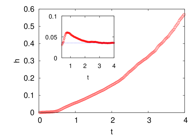
Figure 5: Evolution of the mixing-layer width $h$ as a function of time $t$ for simulation B computed from the profiles of Fig. 4 with a threshold $s=0.8$. The inset shows the compensation with dimensional prediction $h/(Agt^{2})$ converging to a value $\simeq 0.036$.

The evolution of the mixing width for $s=0.8$ is shown in Fig. 5. After an initial stage ($t<0.3\,\tau$) in which the perturbation relaxes towards the most unstable direction, we observe a short exponential growth corresponding to the linear RT instability. At later times ($t>0.6\,\tau$) the similarity regime sets in and the dimensional $t^{2}$ law is observed. The naïve compensation with $Agt^{2}$ gives an asymptotic constant value $h/(Agt^{2})\simeq 0.036$ for $t\geq 3\,\tau$ and $Re\simeq 10^{4}$ (at which the mixing width is still below half box). For the calculation of $\alpha$, more sophisticated analysis have been proposed recently Cabot and Cook (2006); Ristorcelli and Clark (2004); Cook et al. (2004). using slightly different approaches (briefly, in Ristorcelli and Clark (2004) a similarity assumption and in Cook et al. (2004) a mass flux and energy balance argument). In both cases, the authors derive for the evolution of $h(t)$ the equation

$$\dot{h}^{2}=4\alpha Agh$$ (7)

which has solution $h(t)=\alpha Agt^{2}+2(\alpha Ah_{0})^{1/2}t+h_{0}$ where $h_{0}$ is the initial width introduced by the perturbation. $\alpha=\dot{h}^{2}/(4Agh)$. The idea is to get rid of the subleading terms and extract the $t^{2}$ contribution at early time by using directly (7) and evaluating $\alpha=\dot{h}^{2}/(4Agh)$.

The growth of the mixing layer width $h(t)$, a geometrical quantity, is accompanied by the growth of the integral scale $L(t)$, a dynamical quantity representing the typical size of the large-scale turbulent eddies. Following Ref. Vladimirova and Chertkov (2008) we define $L$ as the half width of the velocity correlation function $f(L)=\langle v_{i}(r)v_{i}(r+L)\rangle/\langle v^{2}\rangle=1/2$. In the turbulent regime the integral scale and the mixing length are linearly related (see Fig 6). A linear fit gives $L/h\simeq 1/17$ and $L/h\simeq 1/42$ for the integral scale based on the vertical and horizontal velocity component respectively, in agreement with the results shown in Vladimirova and Chertkov (2008) (of course, the precise values of the coefficients depend on the definition of $h$). The anisotropy of the large scale flow is reflected in the velocity correlation length: the integral scale based on horizontal velocity is smaller than the one based on vertical velocity.

Figure 6: Growth of the integral scale $L$ based on the vertical velocity (red circles), and horizontal velocities (blue squares) as a function of the mixing layer $h$. Data from simulation B.

We end this Section by discussing the behavior of the turbulent heat flux, the energy transfer and the mean temperature gradient in terms of dimensionless variables (as discussed in Sec II): Nusselt, Reynolds and Rayleigh numbers, respectively. The temporal evolution of these numbers, shown in Fig. 7, follows the dimensional predictions (3) for the temporal evolution of $\alpha$ (see Inset of Fig. 5). The presence of the “ultimate state of thermal convection”, in the restricted case $Pr=1$, is also confirmed by our numerical results. Data obtained from simulations at various resolution (see Fig. 8) are in close agreement with the “ultimate state” scalings (4).

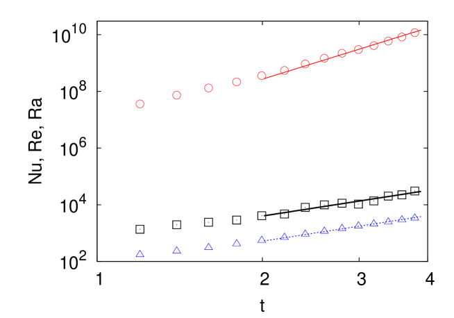
Figure 7: Temporal scaling of Nusselt number $Nu=1+\langle wT\rangle h/(\kappa\theta_{0})$ (blue triangles), Reynolds number $Re=v_{rms}h/\nu$ (black squares) and Rayleigh number $Ra=\beta g\theta_{0}h^{3}/(\nu\kappa)$ (red circles) for simulation $B$ at $Pr=1$. The lines are the temporal scaling predictions $t^{3}$ for $Nu$ and $Re$ and $t^{6}$ for $Ra$.

Figure 8: Nusselt (blue empty symbols) and Reynolds (black filled symbols) numbers as a function of Rayleigh number at $Pr=1$. The “ultimate state” prediction (black and blue lines) expressed by (4) are compared with numerical data obtained from simulations A (squares), B (circles) and C (triangles).

V Small-scale statistics

As already discussed in the introduction, the phenomenological theory predicts that, at small-scales, RT turbulence realizes an adiabatically evolving Kolmogorov–Obukhov scenario of NS turbulence. Here adiabatic means that, because of the scaling laws, small scales have sufficient time to adapt to the variations of large scales, leading to a scale-independent energy flux. We remark that this is not the only possibility, as in two dimensions the phenomenology is substantially different. Unlike the 3D configuration, the 2D scenario is an example of active scalar problem. Indeed, the buoyancy effect is leading at both large and smaller scales. An adiabatic generalization of Bolgiano–Obukhov scaling has been predicted by means of mean field theory Chertkov (2003) and has been confirmed numerically Celani et al. (2006).

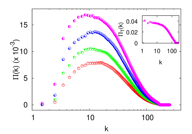
Figure 9: Spectral global kinetic energy flux $\Pi(k)$ at times $t=2.4\tau$, $t=2.6\tau$, $t=2.8\tau$, $t=3.0\tau$ (from bottom to top) and temperature variance flux at $t=3.0\tau$ (inset) for simulation B. Kinetic energy flux is defined as $\Pi(k)=-\int_{k}^{\infty}Re\left[\hat{v}_{i}(-\bf{k}^{\prime})\widehat{({\bf v}\cdot\nabla{v_{i}})}({\bf k}^{\prime})\right]d{\bf k}^{\prime}$ where $\hat{}\,$ is the Fourier transform Frisch (1995). A similar definition holds for the temperature variance flux.

Figure 9 shows the global energy flux in spectral space at different times in the turbulent stage of the simulation. As discussed above, the flux grows in time following the increase of the input $\mathcal{I}(t)$ at large scales and at smaller ones, faster scales have time to adjust their intensities to generate a scale independent flux.

If the analogy with NS turbulence is taken seriously, one can extend the dimensional predictions (5-6) to include intermittency effects. Structure functions for velocity and temperature fluctuations are therefore expected to follow

$$S_{p}(r,t) \equiv \langle(\delta_{r}v_{\parallel}(t))^{p}\rangle\simeq v_{rms}(t)^{p}\left({r\over h(t)}\right)^{\zeta_{p}}$$ (8)

$$S^{T}_{p}(r,t) \equiv \langle(\delta_{r}\theta(t))^{p}\rangle\simeq\theta_{0}^{p}\left({r\over h(t)}\right)^{\zeta^{T}_{p}}$$ (9)

In (8) we introduce the longitudinal velocity differences $\delta_{r}v_{\parallel}(t)\equiv({\bf v}({\bf x}+{\bf r},t)-{\bf v}({\bf x},t))\cdot{\bf r}/r$ and the increment $r$ is made dimensionless with a characteristic large scale which, in the present setup, is proportional to the width of the mixing layer $h(t)$, the only scale present in the system. The two sets of scaling exponents $\zeta_{p}$ and $\zeta^{T}_{p}$ are known from both experiments Warhaft (2000); Moisy et al. (2001) and numerical simulations Watanabe and Gotoh (2004) with good accuracy for moderate $p$. Mean-field prediction is $\zeta_{p}=\zeta^{T}_{p}=p/3$ while intermittency leads to a deviation with respect to this linear behavior. Kolmogorov’s “4/5” law for third-order velocity implies the exact result $\zeta_{3}=1$, while temperature exponents are not fixed, apart for standard inequality requirements Frisch (1995). Both experiments and simulations give stronger intermittency in temperature than in velocity fluctuations, i.e. $\zeta^{T}_{p}<\zeta_{p}$ for large $p$.

We have computed velocity and temperature structure functions and spectra in our simulations of RT turbulence. To overcome the inhomogeneity of the setup, velocity and temperature differences (at fixed time) are taken between points both belonging to the mixing layer as defined above. Isotropy is recovered by averaging the separation ${\bf r}$ over all directions. Spectra are computed by Fourier-transforming velocity and temperature fields on two-dimensional horizontal planes and then averaging vertically over the mixing layer.

V.1 Lower-order statistics

(a)	(b)

Figure 10: (a) Kinetic-energy spectra compensated with $\epsilon^{2/3}$ at times $t=1\tau$ (red crosses), $t=1.4\tau$ (green times), $t=1.8\tau$ (blue stars) and $t=3.8\tau$ (pink squares). Inset: kinetic-energy dissipation vs. time. The line represents the linear growing of energy dissipation (see Sec. II). (b) Temperature-variance spectra compensated with $\epsilon_{T}^{-1}\epsilon^{1/3}$ at same times. Inset: temperature-variance dissipation vs. time. The line is the dimensional prediction $\sim t^{-1}$ (see Sec. II). Data from simulation B.

Figure 11: Third-order isotropic longitudinal velocity structure function $S_{3}(r)$ computed at a late stage in the simulation (red circles) and mixed longitudinal velocity-temperature structure function $S_{1,2}(r)$ (blue triangles). The black line represents the linear scaling. Data from simulation B.

In Fig. 10(a), we plot kinetic-energy spectra at different times in the turbulent stage, compensated with the time dependent energy dissipation $\epsilon^{2/3}(t)$. In the intermediate range of wavenumbers, corresponding to inertial scales, the collapse is almost perfect. The evolution of the compensated spectra shows that the growth of the integral scale at small wavenumbers is in agreement with Fig. 6. Likewise temperature-variance spectra are considered in Fig. 10(b). Here, the spectra are compensated with both the time dependent temperature variance dissipation $\epsilon_{T}^{-1}(t)$ and the energy dissipation $\epsilon^{1/3}(t)$. The evolution of the intermediate range of wavenumbers follows the dimensional prediction (6).

Figure 11 displays the third-order velocity structure function $S_{3}(r)$, related to the energy flux by Kolmogorov’s “4/5” law $S_{3}(r)=-(4/5)\epsilon\,r$ Frisch (1995). We also plot the mixed velocity-temperature structure function $S_{1,2}(r)\equiv\langle\delta_{r}v_{\parallel}(\delta_{r}T)^{2}\rangle$ which is proportional to the (constant) flux of temperature fluctuations $\epsilon_{T}$ according to Yaglom’s law $S_{1,2}(r)=-(4/3)\epsilon_{T}\,r$ Yaglom (1949). Both the computed structure functions display a range of linear scaling, i.e. a constant flux, in the inertial range of scales $5\times 10^{-3}\leq r/L_{z}\leq 5\times 10^{-2}$. It is interesting to observe that the mixed structure function $S_{1,2}(r)$ seems to have a range of scaling which extends to larger scales. This is probably due to the fact that at large-scale temperature fluctuations are dominated by unmixed plumes which have strong correlations with vertical velocity.

Figure 12: Structure-function scaling exponents for velocity increments $\zeta_{p}$ (circles) and temperature increments $\zeta^{T}_{p}$ (triangles) with absolute values. Red open symbols are obtained using ESS procedure Benzi et al. (1993) on the present simulation at time $t=3\,\tau$, fixing the value of $\zeta_{3}=1$ and $\zeta^{T}_{2}=2/3$. Errors represent fluctuations observed in different realizations of simulation B. Blue filled symbols are taken from a stationary NS simulation at $R_{\lambda}=427$ Watanabe and Gotoh (2004). Black line is Kolmogorov non-intermittent scaling $p/3$. Insets: probability density function for velocity differences $\delta_{r}v(t)$ (upper) and temperature differences $\delta_{r}T(t)$ at time $t=3\tau$ and scales $r=0.008L_{z}$ (red circles) and $r=0.06L_{z}$ (green squares). Black lines represent a standard Gaussian.

V.2 Spatial/temporal intermittency

Despite the clear scaling observable in Fig. 11, it is very difficult to compute scaling exponents directly from higher-order structure functions because of limited Reynolds number and statistics. Therefore, assuming a scaling region as in Fig. 11, we can compute relative scaling exponents using the so-called Extended Self Similarity procedure Benzi et al. (1993). This corresponds to consider the scaling of one structure function with respect to a reference one (e.g. $S_{3}(r)$ for velocity statistics), and thus to measure a relative exponent (i.e. $\zeta_{p}/\zeta_{3}$).

Scaling exponents obtained in this way are shown in Fig. 12. Reference exponents for the ESS procedure are $\zeta_{3}=1$ and $\zeta^{T}_{2}=2/3$ (which is not an exact result). We see that both velocity and temperature scaling exponents deviate from the dimensional prediction of (5-6) (i.e. $\zeta_{p}=\zeta^{T}_{p}=p/3$) indicating intermittency in the inertial range. We also observe a stronger deviation for temperature exponents, which is consistent with what is known for the statistics of a passive scalar advected by a turbulent flow Frisch (1995); Sreenivasan and Antonia (1997).

The question regarding the universality of the set of scaling exponents with respect to the geometry and the large-scale forcing naturally arises. Several experimental and numerical investigations in three-dimensional turbulence support the universality scenario in which the set of velocity and passive-scalar scaling exponents are independent of the details of large-scale energy injection and geometry of the flow. Therefore, because we have seen that in 3D RT turbulence at small scales temperature becomes passively transported and isotropy is recovered, one is tempted to compare scaling exponents with those obtained in NS turbulence. As shown in Fig. 12, the two sets of exponents coincide, within the error bars, with the exponents obtained from a standard NS simulation with passive scalar at comparable $R_{\lambda}$ Watanabe and Gotoh (2004).

We remark that scaling exponents for passive scalar in NS turbulence are very sensitive to the fitting procedure. Strong temporal fluctuations have been observed in single realization Chen and Chao (1997) and dependence on the fitting region has been reported Watanabe and Gotoh (2004). Indeed, different realizations of RT turbulence (starting with slightly different initial perturbations) lead to fluctuations of scaling exponents which account for the errorbars shown in Fig. 12.

Figure 12 also shows probability density functions for velocity and temperature fluctuations for two different scales. Both distributions are close to a Gaussian at large scale and develop wide tails at small scales, indicating the absence of self-similarity thus confirming the intermittency scenario.

Figure 13: Time dependence of $p$-order velocity structure function $S_{p}(r_{0},t)$ vs. $S_{2}(r_{0},t)$ for $p=4$ (red open circles) and $p=8$ (blue filled circles) with $r_{0}/L_{z}=0.012$, in the middle of the inertial range for simulation B. Red, continuous lines represent the intermittent prediction $\beta_{p}=p-2\zeta_{p}$ with $\zeta_{p}$ given by spatial structure functions; blue dashed lines are the non-intermittent prediction $\beta_{p}=p/3$.

As a further numerical support of (8-9) we now consider temporal behavior of structure functions. From (8), taking into account the temporal evolution of large scale quantities, we expect the temporal scaling $S_{p}(t)\sim t^{\beta_{p}}$ with $\beta_{p}=p-2\zeta_{p}$. With Kolmogorov scaling one simply has $\beta_{p}=p/3$ but intermittent corrections are expected to be important, for example $\beta_{6}\simeq 2.4$ instead of $p/3=2$. Figure 13 shows the scaling of $S_{p}(r,t)$ vs. $S_{2}(r,t)$ (i.e. in the ESS framework) for a particular value of $r=r_{0}=0.0012L_{z}$. The relative temporal exponents $\beta_{p}/\beta_{2}$ obtained from the spatial exponents $\zeta_{p}$ of Fig. 12 fit well the data, while non-intermittent relative scaling exponents $\beta_{p}/\beta_{2}=p/2$ are ruled out.

The effects of intermittency are particularly important at very small scales. One important example is the statistics of acceleration which has recently been the object of experimental and numerical investigations La Porta et al. (2001); Biferale et al. (2004). For completeness, we briefly recall the main results obtained in those studies.

The acceleration $a$ of a Lagrangian particle transported by the turbulent flow is by definition given by the r.h.s of (1). In the present case of Boussinesq approximation, the acceleration has three contributions: pressure gradient, viscous dissipation and buoyancy terms. Neglecting intermittency for the moment, dimensional scaling (5-6) implies that $-\nabla p\simeq\nu\triangle u\simeq\nu^{-1/4}(\beta g\theta_{0})^{3/2}t^{3/4}$ while $\beta gT\simeq\beta g\theta_{0}$. Therefore the buoyancy term in (1) becomes subleading not only going to small scales but also at later times. Among the other two terms, we find that, as in standard NS turbulence, the pressure gradient term is by far the dominant one, as shown in the inset of Fig. 14. After an initial transient, we have that for $t\geq 2\,\tau$ both terms grow with a constant ratio $(\partial_{z}p)_{rms}/(\nu\triangle w)_{rms}\simeq 8$.

Figure 14: Probability density function of the vertical component of the acceleration at time $t=1\,\tau$ (red, bottom tails), $t=2\,\tau$ (green, intermediate tails) and $t=3.8\,\tau$ (blue, upper tails) normalized with rms values. Inset: evolution of $a_{rms}$ with time for the three contributions of (1): pressure gradient $\partial_{z}p$ (red circles), dissipation $\nu\triangle w$ (green open triangles) and buoyancy term $\beta gT$ (blue filled triangles). Data from simulation B.

The inset of Fig. 14 suggests that the temporal growth of $a_{rms}$ is faster than $t^{3/4}$. Again, this can be understood as an effect of intermittency which is particularly important at small scales. Indeed, using the multifractal model of intermittency Frisch (1995) one obtains the prediction $a_{rms}\sim t^{0.86}$ Biferale et al. (2004).

The effect of intermittency on acceleration statistics is evident by looking at the probability density function. Figure 14 shows that the distribution develops larger tails as turbulence intensity, and Reynolds number, increases. This effect is indeed expected, as the shape of the acceleration pdf depends on the Reynolds number and therefore no universal form is reached. Nevertheless, given the value of $R_{\lambda}$ as a parameter, the pdf can be predicted again using the multifractal model Biferale et al. (2004).

VI Conclusion

We have studied spatial and temporal statistics of Rayleigh–Taylor turbulence in three dimensions at small Atwood number and at Prandtl number one on the basis of a set of high resolution numerical simulations. RT turbulence is a paradigmatic example of non-stationary turbulence with a time dependent injection scale. The phenomenological theory proposed by Chertkov Chertkov (2003) is based on the notion of adiabaticity where small scales are slaved to large ones: the latter are forced by conversion of potential energy into kinetic energy; the former undergo a turbulence cascade flowing to smaller scales until molecular viscosity becomes important. In this picture, temperature actively forces hydrodynamic degrees of freedom at large scales while it behaves like a passive scalar field at small scales where a constant kinetic energy flux develops.

The above scenario suggests comparison of RT turbulence with classical homogeneous, isotropic, stationary Navier–Stokes turbulence, in the general framework of the existence of universality classes in turbulence.

By means of accurate direct numerical simulations, we provide numerical evidence in favor of the mean-field theory. Moreover, we extend the analysis to higher order statistics thus addressing the issue related to intermittency corrections. By measuring scaling exponents of both velocity and temperature structure functions, we find that indeed they are compatible with those obtained in standard turbulence. This result gives further support for the universality scenario.

We also investigate temporal evolution of global quantities, both geometrical (the width of mixing layer) and dynamical (the heat flux). The relevant dimensionless quantity in RT turbulence are the Rayleigh, Reynolds and Nusselt numbers for which there exists an old prediction due to Kraichnan Kraichnan (1962), known as the “ultimate state of thermal convection”, which links the dimensionless number in terms of simple scaling laws. Our set of numerical simulations give again strong evidence for the validity of such scaling in RT turbulence at small Atwood number and at Prandtl number one thus confirming how important in thermal convection is the role of boundaries which prevent the emergence of the ultimate state.

References

- Rayleigh (1883) L. Rayleigh, Proc. London. Math. Soc 14, 170 (1883).
- Taylor (1950) G. Taylor, Proc. Roy. Soc. London 201, 192 (1950).
- Cabot and Cook (2006) W. Cabot and A. Cook, Nature Physics 2, 562 (2006).
- Zingale et al. (2005) M. Zingale, S. E. Woosley, J. B. Bell, M. S. Day, and C. A. Rendleman, Astrophys. J. 632, 1021 (2005).
- Regan et al. (2002) S. P. Regan, J. A. Delettrez, F. J. Marshall, J. M. Soures, V. A. Smalyuk, B. Yaakobi, R. Epstein, V. Y. Glebov, P. A. Jaanimagi, D. D. Meyerhofer, et al., Phys. Rev. Lett. 89, 085003 (2002).
- Fujioka et al. (2004) S. Fujioka, A. Sunahara, K. Nishihara, N. Ohnishi, T. Johzaki, H. Shiraga, K. Shigemori, M. Nakai, T. Ikegawa, M. Murakami, et al., Phys. Rev. Lett. 92, 195001 (2004).
- Chertkov (2003) M. Chertkov, Phys. Rev. Lett. 91, 115001 (2003).
- Frisch (1995) U. Frisch, Turbulence: The Legacy of AN Kolmogorov (Cambridge University Press, Cambridge, 1995).
- Vladimirova and Chertkov (2008) N. Vladimirova and M. Chertkov, Phys. Fluids 21, 015102 (2008).
- Matsumoto (2009) T. Matsumoto, Phys. Rev. E 79, 055301 (2009).
- Boffetta et al. (2009) G. Boffetta, A. Mazzino, S. Musacchio, and L. Vozella, Phys. Rev. E 79, 065301 (2009).
- Zhou (2001) Y. Zhou, Phys. Fluids 13, 538 (2001).
- Siggia (1994) E. Siggia, Ann. Rev. Fluid Mech. 26, 137 (1994).
- Glazier et al. (1999) J. Glazier, T. Segawa, A. Naert, and M. Sano, Nature 398, 307 (1999).
- Niemela et al. (2000) J. Niemela, L. Skrbek, K. Sreenivasan, and R. Donnelly, Nature 404, 837 (2000).
- Xu et al. (2000) X. Xu, K. M. S. Bajaj, and G. Ahlers, Phys. Rev. Lett. 84, 4357 (2000).
- Nikolaenko and Ahlers (2003) A. Nikolaenko and G. Ahlers, Phys. Rev. Lett. 91, 084501 (2003).
- Grossmann and Lohse (2000) S. Grossmann and D. Lohse, J. Fluid Mech. 407, 27 (2000).
- Kraichnan (1962) R. H. Kraichnan, Phys. Fluids 5, 1374 (1962).
- Doering and Constantin (1996) C. R. Doering and P. Constantin, Phys. Rev. E 53, 5957 (1996).
- Lohse and Toschi (2003) D. Lohse and F. Toschi, Phys. Rev. Lett. 90, 034502 (2003).
- Celani et al. (2006) A. Celani, A. Mazzino, and L. Vozella, Phys. Rev. Lett. 96, 134504 (2006).
- Ramaprabhu et al. (2005) P. Ramaprabhu, G. Dimonte, and M. Andrews, J. Fluid Mech. 536, 285 (2005).
- Ramaprabhu and Andrews (2004) P. Ramaprabhu and M. Andrews, J. Fluid Mech. 502, 233 (2004).
- von der Heydt et al. (2003) A. von der Heydt, S. Grossmann, and D. Lohse, Phys. Rev. E 67, 046308 (2003).
- Kuczaj et al. (2008) A. K. Kuczaj, B. J. Geurts, D. Lohse, and W. van de Water, Computer & Fluids 37, 816 (2008).
- Cook and Dimotakis (2001) A. Cook and P. Dimotakis, J. Fluid Mech. 443 (2001).
- Dalziel et al. (1999) S. Dalziel, P. Linden, and D. Youngs, J. Fluid Mech. 399, 1 (1999).
- Ristorcelli and Clark (2004) J. Ristorcelli and T. Clark, J. Fluid Mech. 507, 213 (2004).
- Cook et al. (2004) A. W. Cook, W. H. Cabot, and P. L. Miller, J. Fluid Mech. 511, 2413 (2004).
- Warhaft (2000) Z. Warhaft, Ann. Rev. Fluid Mech. pp. 203–240 (2000).
- Moisy et al. (2001) F. Moisy, H. William, J. S. Andersen, and P. Tabeling, Phys. Rev. Lett. 86, 4827 (2001).
- Watanabe and Gotoh (2004) T. Watanabe and T. Gotoh, New J. of Phys. 6, 40 (2004).
- Yaglom (1949) A. M. Yaglom, Dokl. Akad. Nauk. SSSR 69, 743 (1949).
- Benzi et al. (1993) R. Benzi, S. Ciliberto, R. Tripiccione, C. Baudet, F. Massaioli, and S. Succi, Phys. Rev. E 48, R29 (1993).
- Sreenivasan and Antonia (1997) K. R. Sreenivasan and R. A. Antonia, Ann. Rev. Fluid Mech. 29, 435 (1997).
- Chen and Chao (1997) S. Chen and N. Chao, Phys. Rev. Lett. 78, 3459 (1997).
- La Porta et al. (2001) A. La Porta, G. A. Voth, A. M. Crawford, J. Alexander, and E. Bodenschatz, Nature 409, 1017 (2001).
- Biferale et al. (2004) L. Biferale, G. Boffetta, A. Celani, B. J. Devenish, A. Lanotte, and F. Toschi, Phys. Rev. Lett. 93, 064502 (2004).