Reconciling the analytic QCD with the ITEP operator product expansion philosophy

Abstract

Analytic QCD models are those versions of QCD in which the running coupling parameter $a(Q^{2})$ has the same analytic properties as the spacelike physical quantities, i.e., no singularities in the complex $Q^{2}$ plane except on the timelike semiaxis. In such models, $a(Q^{2})$ usually differs from its perturbative analog by power terms $\sim(\Lambda^{2}/Q^{2})^{k}$ for large momenta, introducing thus nonperturbative terms $\sim(\Lambda^{2}/Q^{2})^{k}$ in spacelike physical quantities whose origin is the UV regime. Consequently, it contradicts the ITEP operator product expansion philosophy which states that such terms can come only from the IR regimes. We investigate whether it is possible to construct analytic QCD models which respect the aforementioned ITEP philosophy and, at the same time, reproduce not just the high-energy QCD observables, but also the low-energy ones, among them the well-measured semihadronic $\tau$ decay ratio.

I Introduction

Today one of the main goals in strong interaction theory is to technically enlarge the applicability of QCD to processes involving lower momentum transfer $q^{2}$. Thereby several obstacles have to be overcome. One of them is that the running QCD coupling $a(Q^{2})={\alpha_{s}(Q^{2})}/{\pi}$, when calculated within the perturbative (“pt”) renormalization group formalism (we call it $a_{\rm pt}$), in the usual (“perturbative”) renormalization schemes, yields singularities of $a_{\rm pt}(Q^{2})$ at $Q^{2}>0$, usually called Landau singularities. Consequently, spacelike observables expressed in terms of powers of $a_{\rm pt}(Q^{2})$ obtain singularities on the spacelike semiaxis $0\leq Q^{2}\leq\Lambda^{2}$ ($Q^{2}=-q^{2}$, with $q$ denoting the typical momentum transfer within a given physical process or quantity). This is not acceptable due to general principles of local quantum field theory BS . Furthermore, studies of ghost-gluon vertex and gluon self-energy using Schwinger-Dyson equations SDEs and large-volume lattice calculations latt , result in QCD coupling $a(Q^{2})$ without Landau singularities at $Q^{2}>0$ and even with a finite value at $Q=0$. Consequently, the behavior of the coupling $a(Q^{2})$ at low values of $Q^{2}$ should be corrected relative to that given by perturbative reasoning.

Several attempts at achieving such corrections have been recorded during the last 14 years starting from (what we call) the minimal analytic (MA) QCD of Shirkov and Solovtsov ShS . Here, the trick lay in simply omitting the wrong (spacelike) part of the branch cut within the dispersion relation formula for $a(Q^{2})$. Consequently, the resulting analytized coupling ${\mathcal{A}}_{1}^{\rm(MA)}(Q^{2})\equiv a^{\rm(MA)}(Q^{2})$ is analytic in the whole Euclidean part of the $Q^{2}$ plane except the nonpositive semiaxis: $Q^{2}\in\mathbb{C}\backslash(-\infty,0]$. Furthermore, for evaluation of physical observables which are represented, in ordinary perturbation theory, as a (truncated) series of powers of $a_{\rm pt}(Q^{2})$, one also has to extend the analytization procedure to $a_{\rm pt}^{n}$ ($n\geq 2$). In MA this was performed in Ref. MSS (see also Ref. Sh ) and resulted in the replacement of $a_{\rm pt}^{n}$ by nonpower expressions ${\mathcal{A}}_{n}^{\rm(MA)}(Q^{2})$. This specific procedure was dubbed by the authors of MSS ; Sh analytic perturbation theory (APT); whereas we will refer to it generally as minimal analytic (MA) QCD.

Other analytic models for $a(Q^{2})$ satisfy certain different or additional constraints at low and/or at high $Q^{2}$ Webber:1998um ; Srivastava:2001ts ; Simonov ; Nesterenko ; Nesterenko2 ; Alekseev:2005he ; CV1 ; CV2 ; CCEM . Analytic QCD models have been used also in the physics of mesons mes1 ; mes2 within the Bethe-Salpeter approach, and in calculation of analytic analogs of noninteger powers $a_{\rm pt}^{\nu}$ Bakulev within the MA model (for reviews of various analytic QCD models, and further references, see Refs. Prosperi:2006hx ; Shirkov:2006gv ; Cvetic:2008bn ). We note that the MA couplings ${\mathcal{A}}_{n}^{\rm(MA)}$ ($n\geq 1$) defined here are the MA couplings of Refs. ShS ; Sh ; Shirkov:2006gv divided by $\pi$.

All of these versions of analytic QCD have one common feature: their (analytized) coupling $a(Q^{2})$ differs from the perturbative coupling even at higher energies by a power term:

$$|\delta a(Q^{2})|\equiv|a(Q^{2})-a_{\rm pt}(Q^{2})|\sim({\Lambda^{2}}/{Q^{2}})^{k}\qquad(Q^{2}\gg\Lambda^{2})\ ,$$ (1)

where $k$ is a positive integer (usually $k=1$; for the models of Refs. Alekseev:2005he ; CCEM : $k=3$). How can these power corrections be interpreted? In a given (usual) renormalization scheme, where $a_{\rm pt}(Q^{2})$ has (Landau) singularities on the positive axis $Q^{2}\sim\Lambda^{2}(\sim 0.1\ {\rm GeV}^{2})>0$, analytization of $a_{\rm pt}(Q^{2})$ can be understood to be achieved by a modification of the discontinuity (“spectral”) function $\rho_{1}^{\rm pt}(\sigma)\equiv{\rm Im}a_{\rm pt}(Q^{2}=-\sigma-i\epsilon)$ at energies $|\sigma|\lesssim\Lambda^{2}$, thereby subtracting the Landau singularities from $a_{\rm pt}(Q^{2})$. It is this subtraction, in the given renormalization scheme, which leads to the power deviations Eq. (1) and, as a consequence, to terms $\sim(\Lambda^{2}/Q^{2})^{k}$ in all spacelike physical quantities. But such contributions are definitely of nonperturbative origin, since they are proportional to $\exp(-K/a_{\rm pt}(Q^{2}))$ which is nonanalytic at $a_{\rm pt}=0$ [cf. Eq. (10) in Sec. II].

Whether such terms, produced in spacelike observables ${\cal D}(Q^{2})$, can be interpreted as being of ultraviolet (UV) origin or not, is not entirely clear. Interpretations of such terms in the literature differ from each other. For example, Ref. Shirkov:1999hm suggests that the Landau pole is not of (entirely) UV origin because the Landau pole persists in the renormalization group resummed expression for $a_{\rm pt}(Q^{2})$ even if one uses, instead of UV logs, the mass-dependent polarization expression (with a sufficiently small gluon mass). On the other hand, the authors of Ref. DMW argue that the aforementioned terms $\sim(\Lambda^{2}/Q^{2})^{k}$ are of UV origin due to the following consideration: If one considers the leading-$\beta_{0}$ summation of an inclusive spacelike observable ${\cal D}(Q^{2})$ (cf. Appendix D)

$${\cal D}^{\rm(LB)}(Q^{2})\equiv\int_{0}^{\infty}\frac{dt}{t}\>F_{\cal D}(t)\>a(tQ^{2}e^{\overline{\cal C}})\ ,$$ (2)

where $F_{\cal D}(t)$ is a characteristic function of the observable and ${\overline{\cal C}}=-5/3$, then the quantity $tQ^{2}e^{\overline{\cal C}}$ indicates the magnitude of the (squares of) internal loop momenta appearing in the resummation. In the UV regime of these momenta, e.g., for $t>1$ (see also Ref. Cvetic:2007ad ), the deviation (1) then leads to power terms of apparently UV origin in the observable

$$\delta{\cal D}^{\rm(LB)}(Q^{2})\sim({\Lambda^{2}}/{Q^{2}})^{k}\int_{1}^{\infty}\frac{dt}{t^{k+1}}\>F_{\cal D}(t)\sim({\Lambda^{2}}/{Q^{2}})^{k}\ .$$ (3)

Considering all these arguments, we come to the conclusion that the aforementioned $(\Lambda^{2}/Q^{2})^{k}$ contributions in physical quantities are at least partially due to UV effects. The existence of nonperturbative contributions stemming from the UV regime is not in accordance with the operator product expansion (OPE) philosophy as advocated by the ITEP group Shifman:1978bx ; DMW . This philosophy rests on the assumption that the OPE, which has originally been derived in perturbation theory (PT), is valid in general (i.e., even when including the nonperturbative contributions) and consequently allows for a separation of short-range from long-range contributions to (inclusive) QCD observables. While the short-range contributions can be calculated perturbatively and lead to expressions for the OPE coefficient functions, the long-range contributions show up as matrix elements of local operators and can be parametrized in terms of condensates (not accessible by PT). And it is this long-range part which leads to power corrections reflecting the contributions of nonperturbative origin to the observable. Therefore, according to the ITEP interpretation, the power term corrections stem from the IR region. This ITEP-OPE approach rests on intuitive physical arguments, and has led to the success of QCD sum rules.

In this work we will adopt the aforementioned ITEP philosophy when analytizing perturbative QCD and, consequently, we will request that the analytic coupling parameter ${\mathcal{A}}_{1}(Q^{2})\equiv a(Q^{2})$ differ from the usual perturbative one at high $Q^{2}$ by less than any power of $\Lambda^{2}/Q^{2}$.

We wish to stress, however, that there is nothing in quantum field theory (QFT) that would impose on us the ITEP interpretation of the OPE. In this context, we mention that the essential singularity at $a=0$ [such as $\exp(-K/a)$] has quite a general and mysterious genesis - first mentioned in QFT by Dyson Dyson1952 on specific physical grounds, and later by many authors on more formal grounds (for an overview, see KSh1980 and references therein).

An additional feature of most versions of analytized QCD is that they fail to reproduce the correct value for the most important (since most reliably measured) QCD observable at low energies, namely $r_{\tau}$, the strangeless semihadronic $\tau$ decay ratio, whose present-day experimental value is (cf. Appendix B): $r_{\tau}({\rm exp.})=0.203\pm 0.004$. Most of the analytic QCD models are either unable to predict unambiguously $r_{\tau}$ value, or they predict significantly smaller values (e.g., in MA, Ref. MSS ; MSSY ), unless unusual additional assumptions are made, e.g., in MA that the light quark masses are much higher than the values of their current masses Milton:2001mq . This finding (loss in the size of $r_{\tau}$) in MA appears to be connected with the elimination of the unphysical (Euclidean) part of the branch cut contribution of perturbative QCD. Since $r_{\tau}$ is the most precisely measured inclusive low momentum QCD observable, its reproduction in analytic QCD models is of high importance. The apparent failure of the MA model with light quark current masses to reproduce the correct value of $r_{\tau}$ had even led to the suggestion that the analytic QCD should be abandoned Geshkenbein:2001mn .

Here, we are investigating whether a modified version of QCD can be defined which simultaneously fulfills the following requirements:

• It is compatible with all analyticity requirements of Quantum Field Theory. In particular, it must not lead to Landau singularities of $a(Q^{2})$, and furthermore we expect (see Sec. II) that $a(Q^{2})$ is analytic at $Q^{2}=0$, and thus IR finite, with $a(Q^{2}=0)\equiv a_{0}<\infty$.

• It is in accordance with the ITEP-OPE philosophy which means that the UV behavior of $a(Q^{2})$ is such that $|a(Q^{2})-a_{\rm pt}(Q^{2})|<(\Lambda^{2}/Q^{2})^{k}$ for any integer $k$ at large $Q^{2}$.

• The theory reproduces the experimental values for $r_{\tau}$ (and other low energetic observables, e.g. the Bjorken polarized sum rule at low $Q^{2}$).

We will show that such a theory is attainable, but only at a certain (acceptable, we think) price. Some of the main results of the present work have been presented, in a summarized form, in Ref. CKV1 .

We are approaching our aim in an indirect way, namely by properly modifying the $\beta$ function $\beta(x)$ $[x=a(Q^{2})]$ of QCD. This approach, which has been used first by Ra̧czka Raczka in a somewhat different context, means that the starting point in the construction is the beta function $\beta(a)$, rather than the coupling parameter $a(Q^{2})$ itself or its discontinuity function $\rho_{1}(\sigma)={\rm Im}a(Q^{2}=-\sigma-i\epsilon)$. The ITEP-OPE condition can be implemented in such an approach in a particularly simple way (see below). Consequently, we are trying to augment $\beta(a)$ which, in general, is only specified by its perturbation series around the point $a=0$

$$\beta(a)=-\beta_{0}a^{2}(1+c_{1}a+c_{2}a^{2}+c_{3}a^{3}+{\cal O}(a^{4}))\ ,$$ (4)

where $\beta_{0}$ and $c_{1}=\beta_{1}/\beta_{0}$ are two universal constants. This should be done in such a way that the augmented beta function leads (via the renormalization group equation RGE) to an effective analytic coupling $a(Q^{2})$ which also enables the correct evaluation of low-energy QCD observables in a perturbative way.

The abovementioned requirements for $a(Q^{2})$ imply the following constraints on the modified beta-function $\beta(a)$:

• The $\beta$ function must be such that the RGE gives a running coupling $a(Q^{2})$ analytic in the entire complex plane of $Q^{2}$, with the possible exception of the nonpositive semiaxis: $Q^{2}\in\mathbb{C}\backslash(-\infty,0]$.

• For small $|a|$, ${\beta}(a)$ has Taylor expansion (4) in powers of $a$, i.e., the perturbative QCD (pQCD) behavior of $\beta(a)$, with universal $\beta_{0}$ and $c_{1}$, at high $Q^{2}$ is attained.

• ${\beta}(a)$ is an analytic (holomorphic) function of $a$ at $a=0$ in order to ensure $|a(Q^{2})-a_{\rm pt}(Q^{2})|<(\Lambda^{2}/Q^{2})^{k}$ for any $k>0$ at large $Q^{2}$ (see Sec. II), thus respecting the ITEP-OPE postulate that powerlike corrections can only be IR induced. At high $Q^{2}$, those pQCD values $a_{\rm pt}(Q^{2})$ which reproduce the known high-energy QCD phenomenology are attained by $a(Q^{2})$.

• It turns out to be difficult or impossible to achieve analyticity (holomorphy) of $a(Q^{2})$ in the Euclidean complex plane $Q^{2}\in\mathbb{C}\backslash(-\infty,0]$ unless the point $Q^{2}=0$ is also included as a point of analyticity of $a(Q^{2})$. This then implies that $a(Q^{2})\to a_{0}$ when $Q^{2}\to 0$, where $a_{0}$ is finite positive, and that $\beta(a)$ has Taylor expansion around $a=a_{0}$ with Taylor coefficient at the first term being unity: ${\beta}(a)=(a-a_{0})+{\cal O}((a-a_{0})^{2})$. Then, $\beta(a)$ is a nonsingular unambiguous function of $a$ in the positive interval $a\in[0,a_{0}]$. Note that analyticity of $a(Q^{2})$ at $Q^{2}=0$ is in full accordance with the general requirement that hadronic transition amplitudes have only the singularities which are enforced by unitarity.

We proceed in this work in the following way. In Sec. II we construct various classes of beta functions which give analytic $a(Q^{2})$ at all $Q^{2}\in\mathbb{C}\backslash(-\infty,0)$ and fulfill the ITEP-OPE condition. We relegate to Appendix A details of the analytic expressions for the implicit solution of RGE and their implications for the (non)analyticity of $a(Q^{2})$. In Sec. III we point out the persistent problem of such models giving too low values of $r_{\tau}$. In Sec. IV we present further modification of the aforementioned beta functions, such that, in addition, the correct value of $r_{\tau}$ is reproduced. In Appendix B we present the extraction of the massless and strangeless $r_{\tau}$ value from experimental data. We relegate to Appendixes C, D and E the presentation of formalisms for the evaluation, in any analytic QCD (anQCD) model, of massless observables, such as the Bjorken polarized sum rule (BjPSR), the Adler function and the related $r_{\tau}$. Appendix C presents construction of the higher order anQCD couplings; Appendix D presents a formalism of resummation of the leading-$\beta_{0}$ (LB) contributions in anQCD; Appendix E presents a calculation of the beyond-the-leading-$\beta_{0}$ (bLB) contributions in anQCD. Section V contains conclusions and outlines prospects for further use of the obtained anQCD models.

II Beta functions for analytic QCD

Our starting point will be the construction of certain classes of beta functions $\beta(a)$ for the coupling $a(Q^{2})$ such that ITEP-OPE conditions

$$|a(Q^{2})-a_{\rm pt}(Q^{2})|<\left(\frac{\Lambda^{2}}{Q^{2}}\right)^{k}\ ,\qquad(k=1,2,\ldots)\ ,$$ (5)

are fulfilled and that, at the same time, they lead to an analytic QCD (anQCD), i.e., the resulting $a(Q^{2})$ is an analytic function for all $Q^{2}\in\mathbb{C}\backslash(-\infty,0]$. This procedure is in contrast to other anQCD models which are usually constructed either via a direct construction of $a(Q^{2})$, or via specification of the discontinuity function $\rho_{1}(\sigma)\equiv{\rm Im}a(Q^{2}=-\sigma-i\epsilon)$ and the subsequent application of the dispersion relation to construct $a(Q^{2})$

$$a(Q^{2})=\frac{1}{\pi}\int_{0}^{+\infty}\ d\sigma\frac{\rho_{1}(\sigma)}{(\sigma+Q^{2})}\ .$$ (6)

In such approaches, it appears to be difficult to fulfill the ITEP-OPE conditions (5) , and difficult or impossible to extract the beta function $\beta(a)$ as a function of $a$.

On the other hand, starting with the construction of a beta function $\beta(a)$, which appears in the RGE

$$Q^{2}\frac{da(Q^{2})}{dQ^{2}}=\beta\left(a(Q^{2})\right)\ ,$$ (7)

it turns out to be simple to fulfill conditions (5) (cf. Ref. Raczka ). Namely, if one requires that $\beta(a)$ be an analytic function of $a$ at $a=0$, then the corresponding $a(Q^{2})$ respects the ITEP-OPE conditions (5).

This statement can be demonstrated in the following indirect way: assuming that the conditions (5) do not hold, we will show that $\beta(a)$ must then be nonanalytic at $a=0$. In fact, if the conditions (5) do not hold, then a positive $n_{0}$ exists such that

$$a(Q^{2})\approx a_{\rm pt}(Q^{2})+\kappa(\Lambda^{2}/Q^{2})^{n_{0}}\,$$ (8)

for $Q^{2}\gg\Lambda^{2}$. Asymptotic freedom of QCD implies that at such large $Q^{2}$ the perturbative $a_{\rm pt}(Q^{2})$ has the expansion (if the conventional, ${\overline{\rm MS}}$, scale $\Lambda={\overline{\Lambda}}$ Buras:1977qg ; Bardeen:1978yd is used)

$$a_{\rm pt}(Q^{2})=\frac{1}{\beta_{0}\ln(Q^{2}/\Lambda^{2})}-\frac{c_{1}}{\beta_{0}^{2}}\frac{\ln\ln(Q^{2}/\Lambda^{2})}{\ln^{2}(Q^{2}/\Lambda^{2})}+{\cal O}\left(\frac{\ln^{2}(\ln(Q^{2}/\Lambda^{2}))}{\ln^{3}(Q^{2}/\Lambda^{2})}\right)\ ,$$ (9)

and consequently the power term can be written as

$$(\Lambda^{2}/Q^{2})^{n_{0}}=\exp\left(-K/a_{\rm pt}(Q^{2})\right)(\beta_{0}a_{\rm pt})^{-K^{\prime}}\left(1+{\cal O}(a\ln^{2}a)\right)\ ,$$ (10)

where $K=n_{0}/\beta_{0}$ and $K^{\prime}=n_{0}c_{1}/\beta_{0}$. Applying $d/d\ln Q^{2}$ to the relation (8) and using expression (10), we obtain

$$\beta(a(Q^{2}))\approx\beta_{\rm pt}(a_{\rm pt}(Q^{2}))-n_{0}\kappa\exp\left(-K/a_{\rm pt}(Q^{2})\right)(\beta_{0}a_{\rm pt})^{-K^{\prime}}\left(1+{\cal O}(a\ln^{2}a)\right)\ .$$ (11)

Replacing $a(Q^{2})$ in the first beta function in Eq. (11) by the right-hand side (rhs) of Eq. (8), using Eq. (10), and Taylor expanding the $\beta(a(Q^{2}))$ function around $a_{\rm pt}(Q^{2})$ ($\not=0$), gives

$$\!\!\!\!\!\!\!\!\!\!\!\!\!\!\!\!\!\!\!\!\!\!\!\!\!\!\!\!\!\!\!\!\beta(a_{\rm pt})+\kappa\exp(-K/a_{\rm pt})(\beta_{0}a_{\rm pt})^{-K^{\prime}}\left(1+{\cal O}(a\ln^{2}a)\right)\times\frac{d\beta(a)}{da}{\big{|}}_{a=a_{\rm pt}}+{\cal O}\left(\exp(-2K/a_{\rm pt})a_{\rm pt}^{-2K^{\prime}}\right)$$ (12)

$$\approx\beta_{\rm pt}(a_{\rm pt})-n_{0}\kappa\exp(-K/a_{\rm pt})(\beta_{0}a_{\rm pt})^{-K^{\prime}}\left(1+{\cal O}(a\ln^{2}a)\right)\ .$$

In this relation, valid for small values of $|a_{\rm pt}|$, the term with derivative $d\beta(a)/da\sim a_{\rm pt}$ on the left-hand side (lhs) can be neglected in comparison with the corresponding term on the rhs. Therefore, Eq. (12) obtains the form (with notation $a_{\rm pt}\mapsto a$)

$$\beta(a)\approx\beta_{\rm pt}(a)-n_{0}\kappa\exp(-K/a)(\beta_{0}a)^{-K^{\prime}}\left(1+{\cal O}(a\ln^{2}a)\right)\ .$$ (13)

We note that $\beta_{\rm pt}(a)$, being a polynomial, is analytic at $a=0$. The term proportional to $\exp(-K/a)$ is nonanalytic at $a=0$, because $\exp(-K/a)$ has an essential singularity there. This shows that nonfulfillment of the ITEP-OPE conditions (5) implies nonanalyticity of $\beta(a)$ at $a=0$, and the demonstration is concluded.

This proof shows that nonfulfillment of ITEP-OPE conditions implies nonfulfillment of $a=0$ analyticity of $\beta(a)$. Or equivalently, fulfillment of $a=0$ analyticity of $\beta(a)$ implies fulfillment of the ITEP-OPE conditions (5). This does not mean the equivalence of $a=0$ analyticity of $\beta(a)$ with the ITEP-OPE conditions. But that will suffice for our purpose, since in the following we will simply restrict the Ansätze for the $\beta$ function which are analytic at $a=0$, thus having the ITEP-OPE conditions secured.

Integration of RGE (7) must be performed for all complex $Q^{2}$. To achieve this, we first need an initial condition [equivalent to the fixing of $\Lambda^{2}$ scale ($\sim 0.1\ {\rm GeV}^{2}$)]. This is a subtle point within our approach, due to two reasons. First, when we choose a specific form of the beta function $\beta(a)$, we automatically choose a specific renormalization scheme (RSch) as well, as represented by the coefficients $c_{j}\equiv\beta_{j}/\beta_{0}$ ($j\geq 2$) of the power expansion of $\beta(a)$, Eq. (4). The running of the corresponding $a(Q^{2})$ can be in general significantly different from the running $a(Q^{2};{\overline{\rm MS}})$ in ${\overline{\rm MS}}$ RSch. Secondly, this running is also influenced by the number of active quark flavors and by flavor threshold effects. In our analyses of RGE with our specific $\beta$ functions, we will consider the number of active quark flavors to be $n_{f}=3$, i.e., the flavors of the three (almost) massless quarks $u$, $d$ and $s$. We do not know how to include in a consistent way the massive quark degrees ($n_{f}\geq 4$) in anQCD. On the other hand, the ITEP-OPE conditions (5) tell us that the considered anQCD theories become practically indistinguishable from pQCD at reasonably high energies $Q^{2}\gg\Lambda^{2}$. Therefore, we wish to keep $n_{f}=3$ in the RGE running to as high values of $|Q^{2}|$ as possible, and to replace the theory at higher $|Q^{2}|$ by pQCD, in the RSch dictated by the specific beta function. Furthermore, in pQCD the threshold for $n_{f}=3\mapsto n_{f}=4$ can be chosen at $Q^{2}\sim(km_{c})^{2}$ with $k\approx 1-3$ BW ; RS ; LRV ; CKS , where $m_{c}$ denotes the mass of the charmed quark. We will use $k=3$, i.e., at $|Q^{2}|\geq(3m_{c})^{2}$ ($\approx 14.5\ {\rm GeV}^{2}$) the anQCD theory will be replaced by pQCD theory.

In order to find the value of $a((3m_{c})^{2})\equiv a_{\rm in}$ which will define our initial condition, we start from the experimentally best known value of the coupling parameter, namely $a(M_{Z}^{2},{\overline{\rm MS}})$. It is deduced, within pQCD, from all relevant experiments at high $|Q^{2}|\gtrsim 10^{1}\ {\rm GeV}^{2}$ and found to be $a(M_{Z}^{2},{\overline{\rm MS}})\approx 0.119/\pi$, Ref. PDG2008 . We RGE run this value, in ${\overline{\rm MS}}$ RSch, down to the scale $(3m_{c})^{2}$, and incorporate the quark threshold matching conditions at the three-loop level according to Ref. CKS at $Q^{2}=3m_{q}^{2}$ ($q=b,c$). We obtain ${\overline{a}}\equiv a((3m_{c})^{2},{\overline{\rm MS}},n_{f}=3)=0.07245$. The value $a_{\rm in}=a((3m_{c})^{2})$, at the same renormalization scale (RScl) but in the RSch as defined by our $\beta(a)$ function, is then obtained from the aformentioned ${\overline{\rm MS}}$ value ${\overline{a}}\equiv a((3m_{c})^{2},{\overline{\rm MS}},n_{f}=3)$ by solving numerically the integrated RGE in its subtracted form (Ref. CK1 , Appendix A there)

$$\frac{1}{a}+c_{1}\ln\left(\frac{c_{1}a}{1\!+\!c_{1}a}\right)+\int_{0}^{a}dx\left[\frac{\beta(x)+\beta_{0}x^{2}(1\!+\!c_{1}x)}{x^{2}(1\!+\!c_{1}x)\beta(x)}\right] = \frac{1}{{\overline{a}}}+c_{1}\ln\left(\frac{c_{1}{\overline{a}}}{1\!+\!c_{1}{\overline{a}}}\right)+\int_{0}^{\overline{a}}dx\left[\frac{{\overline{\beta}}(x)+\beta_{0}x^{2}(1\!+\!c_{1}x)}{x^{2}(1\!+\!c_{1}x){\overline{\beta}}(x)}\right],$$ (14)

where $a\equiv a((3m_{c})^{2})=a_{\rm in}$ and ${\overline{a}}\equiv a((3m_{c})^{2},{\overline{\rm MS}})=0.07245$, both with $n_{f}=3$; further, ${\overline{\beta}}$ is the beta function of the ${\overline{\rm MS}}$ scheme. We note that in Eq. (14) our beta functions have expansions around $a=0$ [cf. Eq. (4)], with the RSch coefficients $(c_{2},c_{3},\ldots)$ which may be considerably different from the ${\overline{\rm MS}}$ coefficients $({\overline{c}}_{2},{\overline{c}}_{3},\ldots)$. Therefore, in Eq. (14) expansions of $\beta$ in powers of $x$ are in general not justified.

Having the initial value $a_{\rm in}=a(Q_{\rm in}^{2}\equiv\mu_{\rm in}^{2}=(3m_{c})^{2})$ fixed, RGE (7) can be solved numerically in the $Q^{2}$-complex plane. It turns out that the numerical integration can be performed more efficiently and elegantly if, instead of $Q^{2}$, a new complex variable is introduced: $z=\ln(Q^{2}/\mu_{\rm in}^{2})$. Then the entire $Q^{2}$-complex plane (the first sheet) corresponds to the semiopen stripe $-\pi\leq{\rm Im}z<+\pi$ in the complex $z$ plane. The Euclidean part $Q^{2}\in\mathbb{C}\backslash(-\infty,0]$ where $a(Q^{2})$ has to be analytic corresponds to the open stripe $-\pi<{\rm Im}(z)<+\pi$; the Minkowskian semiaxis $Q^{2}\leq 0$ is the $z$ line ${\rm Im}z=-\pi$; the point $Q^{2}=0$ corresponds to $z=-\infty$; $Q^{2}=\mu_{\rm in}^{2}$ ($=(3m_{c})^{2}\approx 14.5\ {\rm GeV}^{2}$) corresponds to $z=0$; see Fig. 1.

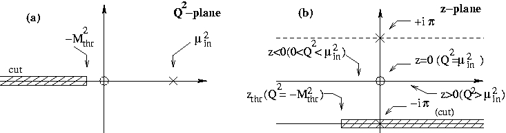
Figure 1: (a) Complex $Q^{2}$ plane; (b) complex $z$ plane where $z=\ln(Q^{2}/\mu_{\rm in}^{2})$; the physical stripe is $-\pi\leq{\rm Im}z<+\pi$.

If we denote $a(Q^{2})\equiv F(z)$, RGE (7) can be rewritten

$$\frac{dF(z)}{dz}=\beta(F(z))\ ,$$ (15)

in the semiopen stripe $-\pi\leq{\rm Im}z<+\pi$. The analyticity requirement for $a(Q^{2})$ now means analyticity of $F(z)$ ($\Rightarrow\partial F/\partial{\bar{z}}=0$) in the open stripe $-\pi<{\rm Im}(z)<+\pi$, and we expect (physical) singularities solely on the line ${\rm Im}(z)=-\pi$. Writing $z=x+iy$ and $F=u+iv$, and assuming analyticity ($\partial F/\partial{\bar{z}}=0$), we can rewrite RGE (15) as a coupled system of partial differential equations for $u(x,y)$ and $v(x,y)$

$$\frac{\partial u(x,y)}{\partial x} = {\rm Re}\beta(u+iv)\ ,\quad\frac{\partial v(x,y)}{\partial x}={\rm Im}\beta(u+iv)\ ,$$ (16)

$$\frac{\partial u(x,y)}{\partial y} = -{\rm Im}\beta(u+iv)\ ,\quad\frac{\partial v(x,y)}{\partial y}={\rm Re}\beta(u+iv)\ .$$ (17)

Thus, beta functions $\beta(F)$ are analytic at $F=0$ [ITEP-OPE condition (5)], and the expansion of $\beta(F)$ around $F=0$ [cf. Eq. (4)] must reproduce the two universal parameters $\beta_{0}$ and $c_{1}=\beta_{1}/\beta_{0}$ (“pQCD condition,” where $\beta_{0}=9/4$ and $c_{1}=16/9$ for $n_{f}=3$), and solution $F(z)=u(x,y)+iv(x,y)$ of RGEs (16)-(17) satisfies the initial condition $F(0)=a_{\rm in}$ where $a=a_{\rm in}$ is determined by Eq. (14).

We implement high precision numerical integration of RGEs (16)-(17) with MATHEMATICA math , for various Ansätze of $\beta(F(z))$ satisfying the aforementioned ITEP-OPE and pQCD conditions. Numerical analyses indicate that it is in general very difficult to obtain analyticity of $F(z)$ in the entire open stripe $-\pi<{\rm Im}(z)<+\pi$, equivalent to the analyticity of $a(Q^{2})$ for all complex $Q^{2}$ except $Q^{2}\in(-\infty,0]$. On the other hand, if we, in addition, require also analyticity of $a(Q^{2})$ at $Q^{2}=0$ ($\Leftrightarrow z=-\infty$), certain classes of $\beta(a)$ functions do give us $F(z)$ with the correct analytic behavior. This $Q^{2}=0$ analyticity condition in general implies

$$a(Q^{2})=a_{0}+a_{1}(Q^{2}/\Lambda^{2})+{\cal O}[(Q^{2}/\Lambda^{2})^{2}]\ ,$$ (18)

where $0<a_{0}\equiv a(Q^{2}=0)=F(z=-\infty)<\infty$ and $a_{1}\not=0$. Application of $d/d\ln Q^{2}=d/dz$ to Eq. (18) then implies that in the Taylor expansion of $\beta(F)$ around $F=a_{0}$ the first coefficient is unity

$$\beta(F)=1\times(F-a_{0})+{\cal O}[(F-a_{0})^{2}]\ ,$$ (19)

or equivalently

$$\beta^{\prime}(F)|_{F=a_{0}}=+1\ .$$ (20)

We write our $\beta(F)$ Ansätze in the form

$$\beta(F)=-\beta_{0}F^{2}(1-Y)f(Y)|_{Y\equiv F/a_{0}}\ ,$$ (21)

with function $f(Y)$ fulfilling the three aforementioned conditions

$$f(Y)\ {\rm analytic\ at}\ Y=0\qquad{\rm(ITEP-OPE)}\ ,$$ (22)

$$f(Y) = 1+(1+c_{1}a_{0})Y+{\cal O}(Y^{2})\qquad{\rm(pQCD)}\ ,$$ (23)

$$a_{0}\beta_{0}f(1) = 1\qquad(Q^{2}=0\ {\rm analyticity})\ .$$ (24)

We always consider $a_{0}$ [$\equiv a(Q^{2}=0)$] to be positive [note: $a=(g_{s}/2/\pi)^{2}>0$].

We will argue in more detail why and how this additional constraint [analyticity of $a(Q^{2})$ at $Q^{2}=0$] improves the analytic behavior of $a(Q^{2})\equiv F(z)$ in the entire $Q^{2}$ plane ($z$ stripe), in the sense of avoiding Landau singularities. For this, it is helpful to consider some simple classes of beta functions which, on the one hand, allow for an implicit analytic solution $z=G(F)$ of RGE (15) and, on the other hand, are representative because larger classes of beta functions can be successively approximated by them. Specifically, we consider $f(Y)$ in Eq. (21) to be either a polynomial or a rational function

$$f(Y) = 1+\sum_{k=1}^{R}r_{k}Y^{k}={\rm P}[R/0]_{f}(Y)\ ,$$ (25)

$$f(Y) = (1+\sum_{k=1}^{M}m_{k}Y^{k})/(1+\sum_{\ell=1}^{N}n_{\ell}Y^{\ell})={\rm P}[M/N]_{f}(Y)\ .$$ (26)

Here, the degrees ($R;M,N$) are in principle arbitrary, and the coefficients ($r_{k};m_{k},n_{\ell}$) as well. Such Ansätze apparently can fulfill all constraints (22)-(24). It is also intuitively clear that they can approximate large classes of other $\beta$ functions that fulfill the same constraints.

Now we undertake the following procedure. Formal integration of RGE (15) leads to the solution

$$z=G(F)\ ,\quad G(F(z))=\int_{a_{\rm in}}^{F(z)}\frac{d{\widetilde{F}}}{\beta({\widetilde{F}})}\ ,$$ (27)

where $a_{\rm in}$ is the aforementioned initial value $a_{\rm in}=a(Q^{2}=\mu^{2}_{\rm in})=F(0)$. Equation (27) represents an implicit (inverted) equation for $F=F(z)=G^{-1}(z)$. In both cases, Eqs. (25) and (26), the integration in Eq. (27) can be performed explicitly. This is performed in Appendix A.

Here we quote, for orientation, the results for two simple examples of $f(Y)$, a quadratic polynomial ${\rm P}[2/0]_{f}$ and a rational function ${\rm P}[1/1]_{f}$.

In the case of quadratic polynomial we have

$$f(Y)=1+r_{1}Y+r_{2}Y^{2}\ ,$$ (28)

where $r_{1}=(1+c_{1}a_{0})$ due to the pQCD condition (23). The (positive) quantity $a_{0}\equiv a(Q^{2}=0)$ is then obtained as a function of the only free parameter $r_{2}$ by the $Q^{2}=0$ analyticity condition (24)

$$a_{0}(r_{2})=\frac{1}{2c_{1}}\left[-(2+r_{2})+\sqrt{(2+r_{2})^{2}+4c_{1}/\beta_{0}}\right]\ .$$ (29)

For the integration (27), we need to rewrite the polynomial (28) in a factorized form

$$f(Y=1/t) = \frac{1}{t^{2}}(t-t_{1})(t-t_{2})\ ,$$ (30)

$$\left(\begin{array}[]{c}t_{1}(r_{2})\\ t_{2}(r_{2})\end{array}\right) = \frac{1}{2}\left[-r_{1}\pm\sqrt{r_{1}^{2}-4r_{2}}\right]\ ,\qquad\left(r_{1}=1+c_{1}a_{0}(r_{2})\right)\ .$$ (33)

Integration (27) then gives the following implicit equation for $F(z)\equiv a(Q^{2})$:

$$z=\left\{\frac{(-1)}{\beta_{0}}\left(\frac{1}{a_{\rm in}}-\frac{1}{F(z)}\right)+\ln\left(\frac{a_{0}/F(z)-1}{a_{0}/a_{\rm in}-1}\right)+\frac{1}{\beta_{0}a_{0}}\sum_{j=1}^{2}B_{j}\ln\left(\frac{a_{0}/F(z)-t_{j}}{a_{0}/a_{\rm in}-t_{j}}\right)\right\}\ ,$$ (34)

where

$$B_{1} = \frac{t_{1}^{3}}{(t_{1}-1)(t_{1}-t_{2})}\ ,\qquad B_{2}=\frac{t_{2}^{3}}{(t_{2}-1)(t_{2}-t_{1})}\ .$$ (35)

In this solution we took into account that the coefficient $B_{0}/(\beta_{0}a_{0}))=1/((1-t_{1})(1-t_{2})(\beta_{0}a_{0}))$ in front of the first logarithm in Eq. (34) is simply unity by the $Q^{2}=0$ analyticity condition (24). The poles $z_{\rm p}$, at which $F(z_{\rm p})=\infty$, are obtained from Eq. (34) by simply replacing $1/F(z)$ by zero

$$z_{\rm p} = \left\{\ln\left(\frac{(-1)}{a_{0}/a_{\rm in}-1}\right)-\frac{1}{\beta_{0}a_{\rm in}}+\frac{1}{\beta_{0}a_{0}}\sum_{j=1}^{2}B_{j}\ln\left(\frac{-t_{j}}{a_{0}/a_{\rm in}-t_{j}}\right)\right\}\ .$$ (36)

It turns out that $a_{0}>a_{\rm in}$ (typically, $a_{0}\approx 0.1$-$0.2$ and $a_{\rm in}<0.1$). If, in addition, $0<r_{2}<r_{1}^{2}/4$, then Eqs. (33) imply $t_{1},t_{2}<0$. Therefore, when $0<r_{2}<r_{1}^{2}/4$, all the arguments in logarithms in Eq. (36) are positive, except in the first logarithm where $\ln(-1)=\pm i\pi$ and thus the only poles of $F(z)$ in the physical stripe ($-\pi\leq{\rm Im}z<\pi$) have

$${\rm Im}z_{\rm p}=-\pi\ .$$ (37)

This implies that for $0<r_{2}<r_{1}^{2}/4$ the considered singularity must lie on the timelike axis ($Q^{2}<0$) and hence does not represent a Landau pole. We stress that for such a conclusion, the $Q^{2}=0$ analyticity condition (24) is of central importance, since it fixes the coefficient in front of $\ln(-1)$ in Eq. (36) to be unity. We can derive from Eq. (36) the location of the pole in the $Q^{2}$ plane at

$$Q^{2}_{\rm p.} = \mu_{\rm in}^{2}\exp(z_{\rm p})=-\mu_{\rm in}^{2}\exp({\rm Re}z_{\rm p})$$ (38)

$$= -\mu_{\rm in}^{2}\exp\left(-\frac{1}{\beta_{0}a_{\rm in}}\right)\left(\frac{a_{0}}{a_{\rm in}}-1\right)^{-1}\prod_{j=1}^{2}\left(\frac{a_{0}/a_{\rm in}-t_{j}}{-t_{j}}\right)^{-B_{j}/(\beta_{0}a_{0})}\ .$$

On the other hand, if the aforementioned conditions are not fulfilled, we obtain $-\pi<{\rm Im}z_{\rm p}<\pi$, representing a pole inside the physical $z$ stripe and thus a Landau singularity. Specifically, when $r_{2}<0$, we have $t_{1}>0$ and $t_{2}<0$ by Eqs. (33); numerically, we can check that in this case always $a_{0}/a_{\rm in}-t_{1}>0$ and, consequently the $j=1$ logarithm in Eq. (36) becomes nonreal and $-\pi<{\rm Im}z_{p}<\pi$, i.e., Landau pole.

To observe in more detail the occurrence and the shape of these singularities, we pursued the numerical solution of RGE (15), i.e., RGEs (16)-(17), accounting for the initial condition at $\mu_{\rm in}^{2}=(3m_{c})^{2}$ in the aforementioned way. In order to see the appearance of singularities of $F(z)\equiv F(x+iy)$ in the physical $z$ stripe, it is convenient to inspect the behavior of $|\beta(F(z))|$ which should show similar singularities. The numerical results for $|\beta(F(z))|$, in the case of $r_{2}=0$ and $r_{2}=-2$ are given in Figs. 2(a), (b), respectively.

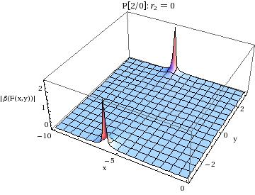
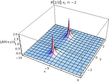
Figure 2: $|\beta(F(z))|$ as a function of $z=x+iy$ for the beta-function (21) with $f(Y)$ having the form (28) with (a) $r_{2}=0$; (b) $r_{2}=-2$.

In these figures, we see clearly that the singularities are on the timelike edge ${\rm Im}z=\pm\pi$ in the case of $r_{2}=0$ where we have $a_{0}=1.901$, $t_{1}\approx-1.338$ [$t_{2}$ is not present as $f(Y)$ is a linear polynomial]. The pole moves inside the $z$ stripe (i.e., become Landau singularities) in the case of $r_{2}=-2$, where we have $a_{0}=0.5$, $t_{1}\approx 0.756$ and $t_{2}\approx-2.645$. In Fig. 3(a) we present the numerical results for the discontinuity function $\rho_{1}(\sigma)={\rm Im}a(Q^{2}=-\sigma-i\epsilon)={\rm Im}F(z=x-i\pi)=v(x,y=-\pi)$ as a function of $x={\rm Re}(z)=\ln(\sigma/\mu^{2}_{\rm in})$, for the case $r_{2}=0$. In Fig. 3(b) the analogous curve for ${\rm Re}a(Q^{2}=-\sigma-i\epsilon)={\rm Re}F(z=x-i\pi)=u(x,y=-\pi)$ is presented, for the same $r_{2}=0$ case. In Figs. 4 (a), (b), the corresponding curves for the $r_{2}=-2$ case are depicted.

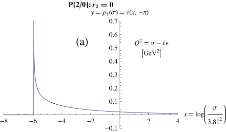
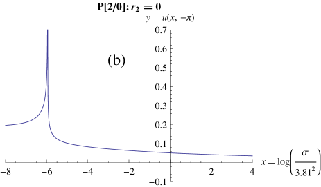
Figure 3: (a) The discontinuity function $\rho_{1}(\sigma)={\rm Im}a(Q^{2}=-\sigma-i\epsilon)={\rm Im}F(z=x-i\pi)=v(x,y=-\pi)$ as a function of $x={\rm Re}(z)=\ln(\sigma/\mu^{2}_{\rm in})$, for the case when $f(Y)$ has the form (28) with $r_{2}=0$, i.e., linear polynomial; (b) same as in (a), but for ${\rm Re}a(Q^{2}=-\sigma-i\epsilon)={\rm Re}F(z=x-i\pi)=u(x,y=-\pi)$.

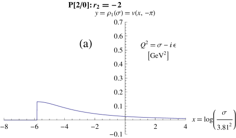
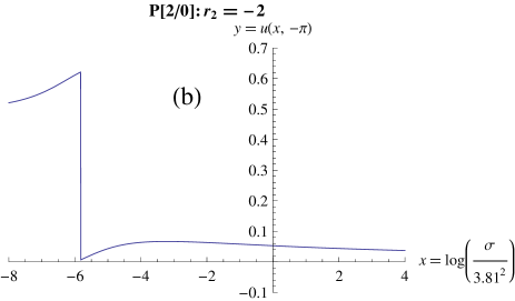
Figure 4: Same as in Figs. 3, but this time $r_{2}=-2$.

We can try many other $f(Y)$ functions, for example, the following set of functions involving (rescaled and translated) functions $(e^{Y}-1)/Y$ and $Y/(e^{Y}-1)$:

$${\rm EE:}\qquad f(Y)=\frac{\left(\exp[-k_{1}(Y-Y_{1})]-1\right)}{[k_{1}(Y-Y_{1})]}\frac{[k_{2}(Y-Y_{2})]}{\left(\exp[-k_{2}(Y-Y_{2})]-1\right)}\times{\cal K}(k_{1},Y_{1},k_{2},Y_{2})\ ,$$ (39)

where the constant ${\cal K}$ ensures the required normalization $f(Y=0)=1$. In this “EE” case we have, at first, five real parameters: $a_{0}\equiv a(Q^{2}=0)$ and four parameters for translation and rescaling ($Y_{1}$, $k_{1}$, $Y_{2}$, and $k_{2}$). Two of the parameters, e.g., $Y_{2}$ and $a_{0}$, are eliminated by conditions (23) and (24). We need $0<k_{1}<k_{2}$ to get physically acceptable behavior and fulfill the aforementioned two conditions. It turns out that, in general, increasing the value of $Y_{1}$ tends to create Landau poles. We consider two typical cases: (1) $y_{1}=0.1;k_{1}=10;k_{2}=11$; (2) $y_{1}=1.1;k_{1}=6;k_{2}=11$. The numerical results for $\beta(F(z))$ for two cases are presented in Figs. 5(a), (b), respectively. We see that the first case shows no sign of Landau poles, while the second case strongly indicates Landau poles.

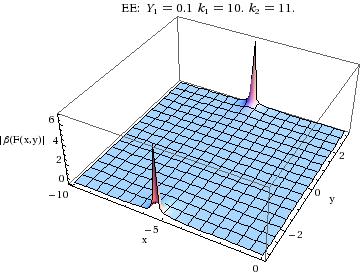
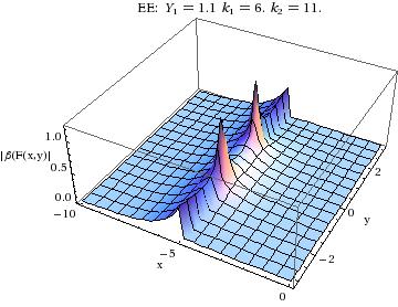
Figure 5: (a) $|\beta(F(z))|$ as a function of $z=x+iy$, where $\beta$ has the form (21) with $f(Y)$ having the EE form (39) with the values of free parameters $y_{1},k_{1},andk_{2}$ as indicated; (b) same as in (a), but with different values of parameters $y_{1}$ and $k_{1}$.

In Figs. 6 and 7 we present the behavior of the imaginary ($v$) and real ($u$) parts of the coupling $F(z=x-i\pi)=a(Q^{2}=-\sigma-i\epsilon)$ along the timelike axis of the $Q^{2}$ plane for the aforementioned two EE cases.

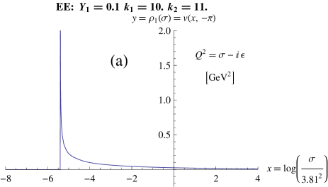
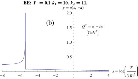
Figure 6: (a) The discontinuity function $\rho_{1}(\sigma)={\rm Im}a(Q^{2}=-\sigma-i\epsilon)={\rm Im}F(z=x-i\pi)=v(x,y=-\pi)$ as a function of $x={\rm Re}(z)=\ln(\sigma/\mu^{2}_{\rm in})$, for the case when $f(Y)$ is the exponential-related EE function (39) with $y_{1}=0.1;k_{1}=10;k_{2}=11$; (b) same as in (a), but for ${\rm Re}a(Q^{2}=-\sigma-i\epsilon)={\rm Re}F(z=x-i\pi)=u(x,y=-\pi)$.

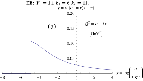
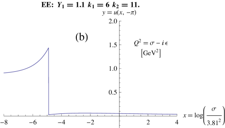
Figure 7: Same as in Figs. 6, but this time $y_{1}=1.1$ and $k_{1}=6$.

There is one interesting feature which can be seen most clearly in Figs. 3(a) and 6(a): the discontinuity function $\rho_{1}(\sigma)\equiv{\rm Im}a(Q^{2}=-\sigma-i\epsilon)$ is zero at negative $Q^{2}$-values above a “threshold” value: $(-M^{2}_{\rm thr}\equiv)$ $-\sigma_{\rm thr}<Q^{2}<0$. For the two cases cited there (“${\rm P}[1/0]$” which is “${\rm P}[2/0]$” with $r_{2}=0$, and EE with $Y_{1}=0.1$), we obtain $x_{\rm thr}=-5.948$ and $-5.403$, respectively, leading to the threshold masses $M_{\rm thr}=195$ MeV and $256$ MeV, respectively. These threshold masses are nonzero and comparable to the low QCD scale $\Lambda_{\rm QCD}$ or pion mass, a behavior that appears physically reasonable. This nonzero threshold behavior (see also Fig. 1) for the discontinuity function $\rho_{1}(\sigma)$ appears because of the $Q^{2}=0$ analyticity requirement for $a(Q^{2})$, Eq. (24). On the other hand, earlier, we saw that the condition Eq. (24) is practically a necessary condition to avoid the appearance of Landau poles of $a(Q^{2})$.

While Figs. 2 and 5 provide only a visual indication of whether the coupling $a(Q^{2})$ is analytic, there is a more quantitative, numerical test for the analyticity. Namely, application of the Cauchy theorem implies for an analytic $a(Q^{2})$, with cut along the negative axis $Q^{2}\leq-M^{2}_{\rm thr}$, the well-known dispersion relation (6) where the integration starts effectively at $\sigma=\sigma_{\rm thr}=M^{2}_{\rm thr}$

$$a(Q^{2})=\frac{1}{\pi}\int_{M_{\rm thr}^{2}}^{+\infty}\ d\sigma\frac{\rho_{1}(\sigma)}{(\sigma+Q^{2})}\ ,$$ (40)

where $\rho_{1}(\sigma)={\rm Im}a(Q^{2}=-\sigma-i\epsilon)$. The high precision numerical solution of RGE (15) gives us $a(Q^{2})=F(z)$ in the entire complex $Q^{2}$ plane, including the negative semiaxis. This allows us to compare numerical values of the lhs and rhs of dispersion relation (40), for various values of $Q^{2}$.

It turns out that, for low positive $Q^{2}\leq 1\ {\rm GeV}^{2}$, the numerical uncertainties of the obtained results for the rhs of Eq. (40) are of the order of per cent (using 64-bit MATHEMATICA math for Linux), and they slowly increase with increasing $Q^{2}$. If the deviation of the rhs from the lhs is more than a few percent, then this represents a strong indication that the resulting $a(Q^{2})$ is not analytic. In Table 1 we present the relative deviations for the aforementioned two ${\rm P}[2/0]$ and the two EE cases. Inspecting these deviations, we can clearly see that $a(Q^{2})$ in the P[2/0] case with $r_{2}=-2$ and the EE case with $Y_{1}=1.1$ is nonanalytic; in the other two cases, the table gives strong indication that $a(Q^{2})$ is analytic.

Table 1: The relative deviation $R[Q^{2}]=({\rm rhs/lhs}-1)$ for the lhs and the rhs of dispersion relation (40) as obtained numerically, for various low positive $Q^{2}$ ($Q^{2}=0.,0.1,1.0\ {\rm GeV}^{2}$), for the aforementioned cases of the beta function.

$f(Y)$	parameters	$R[Q^{2}=0.0]$	$R[Q^{2}=0.1]$	$R[Q^{2}=1.0]$
P[2/0]	$r_{2}=0.0$	$3.3\times 10^{-3}$	$4.6\times 10^{-3}$	$7.0\times 10^{-3}$
P[2/0]	$r_{2}=-2.0$	$-0.62$	$-0.38$	$-0.09$
EE	$Y_{1}=0.1,k_{1}=10.0,k_{2}=11.0$	$4.7\times 10^{-3}$	$4.8\times 10^{-3}$	$6.5\times 10^{-3}$
EE	$Y_{1}=1.1,k_{1}=6.0,k_{2}=11.0$	$-0.82$	$-0.68$	$-0.19$

III Evaluation of low-energy observables

The semihadronic $\tau$ decay ratio $R_{\tau}$ is the most precisely measured low-energy QCD quantity to date. The measured value of the “QCD-canonical” part $r_{\tau}=a+{\cal O}(a^{2})$, with the strangeness and quark mass effects subtracted, is $r_{\tau}^{\rm(exp)}=0.203\pm 0.004$ (cf. Appendix B). Experimental values of other low-energy observables, such as (spacelike) sum rules, among them the Bjorken polarized sum rule (BjPSR) $d_{\rm Bj}(Q^{2})$, are known with far less precision. The minimal analytic (MA) model ShS ; MSS ; Sh ; Shirkov:2006gv , with the value of ${\overline{\Lambda}}$ such that high-energy QCD observables are reproduced, turns out to give for this quantity too low values $r_{\tau}\approx 0.14$ MSS ; MSSY unless the (current) masses of the light quarks are taken to be unrealistically large ($m_{q}\approx 0.25$-$0.45$ GeV) or strong threshold effects are introduced Milton:2001mq . Further, MA does not fulfill the ITEP-OPE condition (5) since $|a^{\rm(MA)}(Q^{2})-a_{\rm pt}(Q^{2})|\sim(\Lambda^{2}/Q^{2})$.

The approach described in the previous Sec. II automatically fulfills the ITEP-OPE condition (5); however, the analyticity of $a(Q^{2})$, i.e., the absence of Landau poles, is achieved only for limited regions of the otherwise free parameters of the $\beta$ function. For general anQCD models, the evaluation of massless spacelike observables ${\cal D}(Q^{2})$ such as BjPSR and Adler function, and for the timelike observable $r_{\tau}$, is presented in the sequence of Appendixes C, D, E, particularly Eqs. (120)-(123) for spacelike and (133)-(136) for $r_{\tau}$. In the cases considered in this work, the beta function $\beta(a)$ is analytic at $a=0$ (due to the ITEP-OPE condition), and therefore the higher order analogs ${\mathcal{A}}_{n+1}$ in those Appendixes are simply ${\mathcal{A}}_{n+1}=a^{n+1}$, cf. Eq. (91). Furthermore, here we use all the time the notation ${\mathcal{A}}_{1}\equiv a$ for the analytic coupling, and ${\widetilde{\mathcal{A}}}_{n+1}\equiv{\widetilde{a}}_{n+1}$ for the logarithmic derivatives of $a$ [cf. Eq. (67)].

In Table 2 we present the resulting values of RSch parameters $c_{2}$, $c_{3}$ and $c_{4}$ [cf. Eq. (4)], for some typical choices of input parameters in four forms of $f(Y)$: P[1/0], P[3/0], P[1/1], and EE. Here, ${\rm P}[M/N]$ is the general notation for Padé form Eq. (45) in Appendix A; ${\rm P}[M/0]$ is thus a polynomial of degree $M$; EE is the Ansatz (39) involving exponential functions. The otherwise free parameters (“input”) of the models are chosen such that the analyticity is maintained, i.e., no Landau poles. The case P[1/0] is in fact the aforementioned case of P[2/0] with $r_{2}=0$, cf. Eq. (28), and it has no free parameters. The cases P[3/0] and P[1/1] have each one free input parameter; for P[3/0] the first root $t_{1}$ is the specified input, and for P[1/1] the first pole $u_{1}$, where the notation (45) of Appendix A is used. The case EE is given in Eq. (39), and has three free parameters. We recall that an apparently additional parameter in the Ansätze for $f(Y)$ is fixed by the pQCD condition (23). In addition, we present the values of $a(Q^{2})$ at the initial condition scale $\mu_{\rm in}^{2}=(3m_{c})^{2}$ ($m_{c}=1.27$ GeV) and at $Q^{2}=0$; and the threshold value $x_{\rm thr}$ of the discontinuity function $\rho_{1}(\sigma)={\rm Im}a(-\sigma-i\epsilon)$, where: $z_{\rm thr}=x_{\rm thr}-i\pi$, $\sigma_{\rm thr}=(3m_{c})^{2}\exp(x_{\rm thr})$. Further, the corresponding threshold mass $M_{\rm thr}$ is given [$M_{\rm thr}=3m_{c}\exp(x_{\rm thr}/2)$].

Table 2: Four cases of $\beta$ function $(f(Y))$, with chosen input parameters. Given are the resulting RSch parameters $c_{n}$ ($n=2,3,$ and $4$), and the values of $a(Q^{2})$ at $Q^{2}=(3m_{c})^{2}$ and $Q^{2}=0$. Further, the resulting threshold parameter $x_{\rm thr}$ and the threshold mass $M_{\rm thr}$ (in GeV) are given. Recall that $a((3m_{c})^{2},{\overline{\rm MS}})=0.07245$.

$f$	Input	$c_{2}$	$c_{3}$	$c_{4}$	$a((3m_{c})^{2})$	$a_{0}\equiv a(0)$	$x_{\rm thr}$	$M_{\rm thr}$ [GeV]
P[1/0]	–	-37.02	0	0	0.06047	0.1901	-5.948	0.195
P[3/0]	$t_{1}=1+i0.45$	-39.55	115.88	-105.80	0.06066	0.4562	-11.092	0.015
P[1/1]	$u_{1}=-0.1$	-37.54	18.84	-9.46	0.06048	0.1992	-6.060	0.184
EE	$Y_{1}=0.1$, $k_{1}=10.0$, $k_{2}=11.0$	-10.80	-157.62	-644.32	0.06544	0.2360	-5.403	0.256

For two of these models (P[1/0], and EE), we depict in Figs. 8 and 9 the form of $f(Y)$ and $\beta(x)$ functions for real values of $Y=a/a_{0}$ and positive values of $x\equiv a>0$, respectively. In Figs. 10-11 we present the running coupling $a(Q^{2})$ as a function of $Q^{2}$ for positive $Q^{2}$ in the two models; there we include, in addition, the higher order analytic couplings ${\widetilde{a}}_{n+1}$ ($n=1,2$).

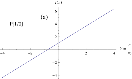
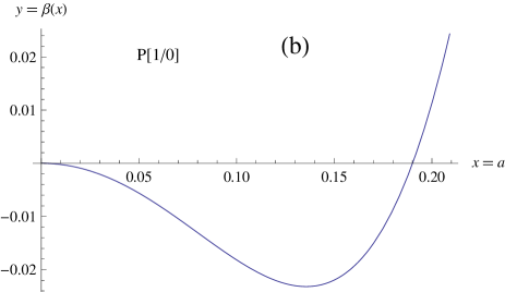
Figure 8: (a) $f(Y)$ function as defined by Eq. (21), for real values of $Y\equiv a/a(0)$, for the case of $f$ being P[1/0] linear function ($\Leftrightarrow$ P[2/0] with $r_{2}=0$); (b) $\beta(x)$ function for the same case, for positive $x\equiv a$.

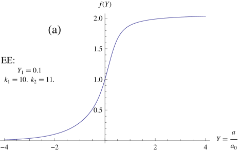
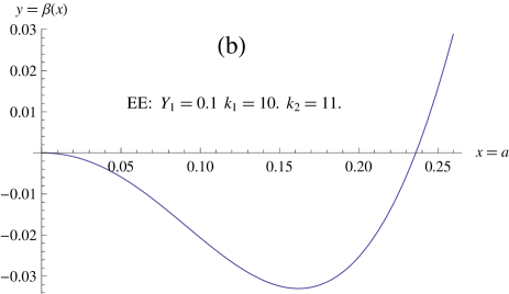
Figure 9: Same as in Fig. 8, but this time $f(Y)$ being the exponential-related function EE, Eq. (39).

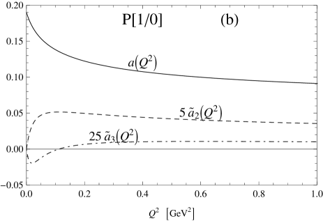
Figure 10: (a) Analytic coupling $a(Q^{2})$ and its higher order analogs ${{\widetilde{a}}}_{n+1}$ ($n=1,2$) as defined in Eq. (67), for positive $Q^{2}$, for the model P[1/0]. For better visibility, the higher order analogs are scaled by factors of $5$ and $5^{2}$, respectively. (b) Same as in (a), but at lower $Q^{2}$. We recall that, formally: ${\widetilde{a}}_{n+1}=a^{n+1}+{\cal O}(a^{n+2})$.

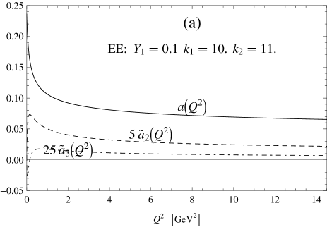
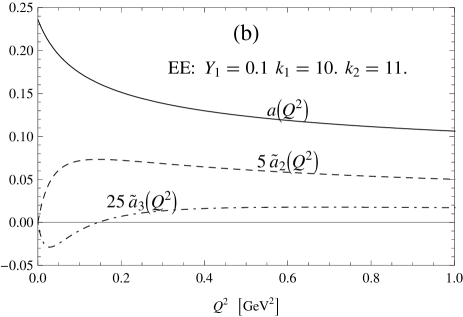
Figure 11: Same as in Fig. 10, but for the model EE, Eq. (39).

The model with $f=$ P[1/0] is, at first sight, very similar to the model of Ref. MS which was obtained on the basis of the principle of minimal (renormalization scheme) sensitivity (PMS) Stevenson applied to the QCD part of $R_{e^{+}e^{-}}(s)$ ratio. There, the beta function is also a polynomial of the fourth degree, i.e., $f(Y)$ is linear, and it has a finite positive value of $a(Q^{2}=0)\equiv a_{0}$. It turns out that for the beta function of Ref. MS the conditions (22) and (23) are fulfilled, but not the condition of $Q^{2}=0$ analyticity Eq. (24). As argued in the present paper, such beta function will give unphysical (Landau) poles, although in this case not on the positive $Q^{2}$ axis. Specifically, for $n_{f}=2$ and $n_{f}=3$ the $Q^{2}=0$ analyticity condition (24) yields in the P[1/0] case the values $a_{0}=0.1761$ and $0.1901$, respectively, while the values of $a_{0}$ in Ref. MS are $a_{0}=0.263$ and $0.244$, respectively. We checked numerically that this PMS solution leads to (Landau) poles of $a(Q^{2})$ at $Q^{2}\approx(-0.027\pm i0.065)\ {\rm GeV}^{2}$ for $n_{f}=2$, and at $Q^{2}\approx(-0.031\pm i0.032)\ {\rm GeV}^{2}$ for $n_{f}=3$ (massless quarks).

Let us now apply these results to calculating low-energy QCD observables.

We start with $r_{\tau}$.

In Table 3 we present the predicted values of $r_{\tau}$ for the choices of $\beta$ functions and input parameters given in Table 2.

Table 3: The four terms in truncated analytic expansions (133) and (135) for $r_{\tau}$, i.e., with LB contributions resummed and the three bLB terms organized in contour integrals of ${\widetilde{\mathcal{A}}}_{n+1}\equiv{\widetilde{a}}_{n+1}$ (first line) and of ${\mathcal{A}}_{n+1}=a^{n+1}$ (second line of each model). In parentheses are the corresponding results when no LB resummation is performed, i.e., the truncated analytic expansions Eqs. (134) and (136), respectively. The RScl parameter is ${\cal C}=0$. The last column contains variations of these truncated sums when the RScl parameter ${\cal C}$ increases from $0$ to $\ln 2$.

$f$	$r_{\tau}:$ LB (LO)	NLB (NLO)	${\rm N}^{2}{\rm LB}$ (${\rm N}^{2}{\rm LO}$)	${\rm N}^{3}{\rm LB}$ (${\rm N}^{3}{\rm LO}$)	Sum (sum)	$\delta$ (${\cal C}$ dependence)
P[1/0]	0.1135(0.0940)	0.0006(0.0123)	0.0139(0.0214)	0.0007(0.0012)	0.1287(0.1289)	$-0.2\%(-0.4\%)$
	0.1135(0.0940)	0.0007(0.0137)	0.0209(0.0340)	0.0091(0.0113)	0.1442(0.1529)	$-2.8\%(-2.7\%)$
P[3/0]	0.1200(0.0954)	0.0007(0.0131)	0.0184(0.0275)	-0.0009(0.0000)	0.1381(0.1360)	$-0.3\%(-0.8\%)$
	0.1200(0.0954)	0.0007(0.0141)	0.0233(0.0369)	0.0067(0.0087)	0.1507(0.1550)	$-2.4\%(-2.9\%)$
P[1/1]	0.1142(0.0941)	0.0006(0.0124)	0.0146(0.0224)	0.0005(0.0011)	0.1300(0.1300)	$-0.2\%(-0.5\%)$
	0.1142(0.0941)	0.0007(0.0138)	0.0213(0.0344)	0.0088(0.0109)	0.1450(0.1532)	$-2.8\%(-2.7\%)$
EE	0.1348(0.1088)	0.0009(0.0173)	0.0025(0.0156)	0.0048(0.0061)	0.1466(0.1478)	$-0.8\%(-1.2\%)$
	0.1348(0.1088)	0.0009(0.0180)	0.0033(0.0224)	0.0102(0.0173)	0.1528(0.1666)	$-2.8\%(-3.7\%)$

Therein we separately give (in each line) the four terms of the truncated analytic series for $r_{\tau}$ and then quote their sum. Furthermore, for each model of $f(Y)$ we present the results for basically two different ways of treating the higher orders. In the first row of each model, the results of the series (133) are presented, which performs leading-$\beta_{0}$ (LB) resummation and adds the (three) beyond-the-leading-$\beta_{0}$ (bLB) terms organized in contour integrals of logarithmic derivatives ${\widetilde{a}}_{n+1}$ ($n=1,2,3$). In the second line, the analogous results are presented, where now the (three) bLB terms are contour integrals of powers ${\mathcal{A}}_{n+1}\equiv a^{n+1}$, Eq. (135). At each of the entries, the corresponding terms are given when no LB resummation is performed, cf. Eqs. (134), (136). The RScl parameter used is ${\cal C}=0$, i.e., the radius of the contour in the $Q^{2}$ plane is $m_{\tau}^{2}$. In the last column, the relative variation of the sum is given when the RScl parameter is increased from ${\cal C}=0$ to $\ln 2$, i.e., the radius of the contour integration is increased to $2m_{\tau}^{2}$. The results using the powers $a^{n+1}$ for the bLB (or: higher order) contributions show significantly less stability under the RScl variation; the reason for this lies in two numerical facts:

• The expansion coefficient $(t_{\rm Adl})_{3}$ of the latter series is usually larger than the corresponding coefficient $(T_{\rm Adl})_{3}$ of the series containing ${\widetilde{a}}_{n+1}$: $|(t_{\rm Adl})_{3}|>|(T_{\rm Adl})_{3}|$; this seems to be true in all the RSch’s dictated by the presented $\beta$ functions.

• Apparently in all cases we have $|{\widetilde{a}}_{n+1}|<|a^{n+1}|$, although formally ${\widetilde{a}}_{n+1}=a^{n+1}+{\cal O}(a^{n+2})$.

Furthermore, the variations of the result under variations of RScl are generally smaller when LB resummation is performed. Therefore, we will consider as our preferred choice the evaluated values of the first lines (not in parentheses) of each model in Table 3, i.e., the evaluations using ${\widetilde{a}}_{n+1}$ for the higher order contributions, i.e., Eq. (133).

We note that the obtained values of $r_{\tau}$ (see the “sum” in Table 3) are all much too low when compared with the experimental value $r_{\tau}^{\rm(exp)}=0.203\pm 0.004$ (cf. Appendix B). In fact, the free parameters in the Ansätze for $f(Y)$ of the beta function were chosen in Tables 2-3 in such a way as to (approximately) maximize the result for $r_{\tau}$ while still maintaining analyticity of $a(Q^{2})$ (i.e., no Landau singularities). We can see that the preferred evaluation method, i.e., the first line of each case, gives us always a value $r_{\tau}<0.15$. We tried many choices for the function $f(Y)$ of Eq. (21), fulfilling all conditions (22)-(24), and scanning over the remaining free parameters in $f(Y)$. It turned out that $r_{\tau}<0.16$ always as long as Landau poles were absent. Only when free parameters were chosen such that Landau poles appeared, was it possible to increase $r_{\tau}$ beyond $0.16$.

As the second example we consider the Bjorken polarized sum rule (BjPSR) $d_{\rm Bj}(Q^{2})$.

In Table 4 we present results for $d_{\rm Bj}(Q^{2})$ in the aforementioned cases, at three of those low values of $Q^{2}$ where experimental results are available: $Q^{2}=1.01$, $2.05$, and $2.92\ {\rm GeV}^{2}$.

Table 4: Bjorken polarized sum rule (BjPSR) results $d_{\rm Bj}(Q^{2})$ for the four considered $\beta$ Ansätze, evaluated with the truncated analytic expansions (120) and (122), i.e., with LB contributions resummed and the three bLB terms $\propto{\widetilde{\mathcal{A}}}_{n+1}\equiv{\widetilde{a}}_{n+1}$ (first line) and $\propto{\mathcal{A}}_{n+1}=a^{n+1}$ (second line). In parentheses are the corresponding results when no LB resummation is performed, i.e., truncated analytic expansions Eqs. (121) and (123), respectively. The RScl parameter is ${\cal C}=0$. In brackets, the corresponding variations of the results under the RScl variation are given (see the text for details). For explanation of the experimental values in the last (four) lines, see the text for details.

$f$	$d_{\rm Bj}(Q^{2}):\ Q^{2}=1.01\ {\rm GeV}^{2}$	$Q^{2}=2.05\ {\rm GeV}^{2}$	$Q^{2}=2.92\ {\rm GeV}^{2}$
P[1/0]	$0.1343[+0.3\%]$ $(0.1420[-1.9\%])$	$0.1208[-0.1\%]$ $(0.1255[-0.5\%])$	$0.1140[-0.2\%]$ $(0.1173[-0.7\%])$
	$0.1535[-4.1\%]$ $(0.1974[-5.1\%])$	$0.1313[+2.8\%]$ $(0.1552[-4.1\%])$	$0.1218[-2.4\%]$ $(0.1393[-3.6\%])$
P[3/0]	$0.1609[-0.4\%]$ $(0.1630[-1.9\%])$	$0.1366[-0.4\%]$ $(0.1361[-2.0\%])$	$0.1261[-0.4\%]$ $(0.1249[-1.9\%])$
	$0.1773[-3.7\%]$ $(0.2053[-6.3\%])$	$0.1456[-2.6\%]$ $(0.1587[-4.6\%])$	$0.1329[-2.2\%]$ $(0.1417[-4.0\%])$
P11	$0.1373[+0.2\%]$ $(0.1450[-1.5\%])$	$0.1226[-0.1\%]$ $(0.1270[-0.6\%])$	$0.1154[-0.2\%]$ $(0.1184[-0.9\%])$
	$0.1561[-4.0\%]$ $(0.1985[-5.3\%])$	$0.1329[-2.8\%]$ $(0.1557[-4.2\%])$	$0.1231[-2.4\%]$ $(0.1396[-3.7\%])$
EE	$0.1507[+0.3\%]$ $(0.1659[-3.7\%])$	$0.1338[+0.1\%]$ $(0.1434[-1.0\%])$	$0.1256[+0.1\%]$ $(0.1324[-1.0\%])$
	$0.1436[+0.7\%]$ $(0.2300[-6.8\%])$	$0.1304[+0.5\%]$ $(0.1725[-5.1\%])$	$0.1232[+0.4\%]$ $(0.1521[-4.4\%])$
Exp. (a):	$0.23\pm 0.18$	$0.11\pm 0.11$	$0.09\pm 0.07$
$\mu_{4}^{\rm p-n}=-0.040\pm 0.028$	$0.23\pm 0.12\pm 0.13$	$0.11\pm 0.09\pm 0.06$	$0.09\pm 0.05\pm 0.05$
Exp. (b):	$0.30\pm 0.18$	$0.15\pm 0.11$	$0.11\pm 0.07$
$\mu_{4}^{\rm p-n}=-0.024\pm 0.028$	$0.30\pm 0.12\pm 0.13$	$0.15\pm 0.09\pm 0.06$	$0.11\pm 0.05\pm 0.05$

As in the previous Table 3, the first line of each model contains the results with our preferred method, i.e., LB resummation and usage of ${\widetilde{a}}_{n+1}$ for the bLB contributions, Eq. (120); the second line represents the results of LB resummation and the usage of $a^{n+1}$ powers for the bLB contributions, Eq. (122). In the parentheses, the corresponding results are given when no LB resummation is performed, Eqs. (121) and (123), respectively. In the corresponding brackets, the variations of the results are given when the RScl parameter varies either from ${\cal C}=0$ ($\mu^{2}=Q^{2}$) to ${\cal C}=\ln 2$ ($\mu^{2}=2Q^{2}$), or from ${\cal C}=0$ to ${\cal C}=\ln(1/2)$ ($\mu^{2}=Q^{2}/2$) – the larger of the variations is given. As in the case of $r_{\tau}$, we see that the most stable evaluation under variations of RScl is the LB resummation and the usage of ${\widetilde{a}}_{n+1}$ for the bLB contributions, Eq. (120).

For comparison, we include in Table 4 (last lines) three sets of experimental data based on the JLab CLAS EG1b (2006) measurements Deur2008 of the $\Gamma_{1}^{\rm p-n}(Q^{2})$ sum rule for spin-dependent proton and neutron structure functions $g_{1}^{\rm p,n}$ Kataev:1994gd . $\Gamma_{1}^{\rm p-n}$ is connected to $d_{\rm Bj}$ in the following way:

$$\Gamma_{1}^{\rm p-n}(Q^{2}) \equiv \int_{0}^{1}\;dx_{\rm Bj}\;\left(g_{1}^{\rm p}(x_{\rm Bj},Q^{2})-g_{1}^{\rm n}(x_{\rm Bj},Q^{2})\right)$$ (41)

$$= \frac{g_{A}}{6}\left(1-d_{\rm Bj}(Q^{2})\right)+\sum_{j=2}^{\infty}\frac{\mu_{2j}^{\rm p-n}(Q^{2})}{(Q^{2})^{j-1}}\ ,$$ (42)

where $g_{A}=1.267\pm 0.004$ PDG2008 is the triplet axial charge, $1-d_{\rm Bj}(Q^{2})=1-a(Q^{2})+{\cal O}(a^{2})$ is the nonsinglet leading-twist Wilson coefficient, and $\mu_{2j}^{\rm p-n}/Q^{2j-2}$ ($j\geq 2$) are the higher-twist contributions. If we take into account the data with the elastic contribution excluded, we can restrict ourselves to the first higher-twist term $\mu_{4}^{\rm p-n}/Q^{2}$. The elastic contribution affects largely only the other higher-twist terms $\sim 1/(Q^{2})^{j-1}$ with $j\geq 3$, as has been noted in Refs. Pase1 ; Pase2 . Moreover, the exclusion of the elastic contribution leads to strongly suppressed higher-twist terms $\sim 1/(Q^{2})^{j-1}$ with $j\geq 3$ Pase1 in pQCD and MA (APT) approaches. The first experimental set (a) for $d_{\rm Bj}(Q^{2})$ in Table 4 is obtained from the measured values of $\Gamma_{1}^{\rm p-n}(Q^{2})$ (with the elastic part excluded) by subtracting the $\mu_{4}^{\rm p-n}/Q^{2}$ contribution as obtained by a 3-parameter pQCD fit Deur2008 : $\mu_{4}^{\rm p-n}\approx\mu_{4}^{\rm p-n}(Q=1{\rm GeV})=-0.040\pm 0.028$; the second set (b) is obtained in the same way, but now by subtracting the $\mu_{4}^{\rm p-n}/Q^{2}$ contribution obtained by a 4-parameter pQCD fit Deur2008 : $\mu_{4}^{\rm p-n}\approx\mu_{4}^{\rm p-n}(Q=1{\rm GeV})=-0.024\pm 0.028$. In the second line of each experimental set, the uncertainties were split into the contribution coming from the uncertainty of the measured value of $\Gamma_{1}^{\rm p-n}(Q^{2})$ and the one from the uncertainty of the fitted value $\mu_{4}^{\rm p-n}$ Deur2008 .

We see from Table 4 that the evaluated values for BjPSR lie in general relatively close to the central experimental values $d_{\rm Bj}(Q^{2})_{\rm exp.}$: $d_{\rm Bj}(Q^{2})_{\rm exp.}=0.23$ (or $0.30$) for $Q^{2}=1.01\ {\rm GeV}^{2}$; $0.11$ (or $0.15$) for $Q^{2}=2.05\ {\rm GeV}^{2}$; $0.09$ (or $0.11$) for $Q^{2}=2.92\ {\rm GeV}^{2}$. However, in contrast to $r_{\tau}$, the experimental uncertainties are now much larger and the theoretical predictions lie well within the large intervals of experimental uncertainties.

IV Tackling the problem of too low $r_{\tau}$

The problem of too low $r_{\tau}$, encountered in the previous Section, appears to be common to all or most of the anQCD models. For example, in the MA of Shirkov, Solovtsov and Milton ShS ; MSS ; Sh ; Shirkov:2006gv ; MSSY , when adjusting ${\overline{\Lambda}}$ to such a value as to reproduce higher energy QCD observables ($Q^{2}\gtrsim 10^{1}\ {\rm GeV}^{2}$), i.e., ${\overline{\Lambda}}\approx 0.4$ GeV, the resulting value of (massless and strangeless) $r_{\tau}$ is about $0.140$-$0.141$ MSS ; MSSY ; CV2 , much too low. The results of the previous section indicate that this problem persists even in anQCD models which, unlike MA, fulfill the ITEP-OPE condition (5). The aspect of anQCD models which appears to cause the tendency toward too low values of $r_{\tau}$ is the absence of (unphysical) Landau cut along the positive $Q^{2}$ axis ($0\leq Q^{2}<Q_{\rm LP}^{2}$). Therefore, we are apparently facing a strange situation:

• In pQCD the Landau cut of the coupling gives a numerically positive contribution to $r_{\tau}$, and pQCD is able to reproduce the experimental value of $r_{\tau}$ (cf. Refs. Geshkenbein:2001mn ; Braaten:1988hc ; Pivovarov:1991rh ; Le Diberder:1992te ; Ball:1995ni ; ALEPH2 ; ALEPH3 ; DDHMZ ; Ioffe ; Beneke:2008ad ; Caprini:2009vf ; DescotesGenon:2010cr ; MY , because of this (unphysical) feature of the theory.

• In anQCD the physically unacceptable low-energy (Landau) singularities of the coupling are eliminated, but then the values of $r_{\tau}$ tend to decrease too much.

Here we indicate one possible solution to this problem (cf. also our shorter version CKV1 ). Table 3 indicates that the LB-resummed contribution to $r_{\tau}$ cannot surpass the values $0.14$-$0.15$. We performed many trials with various forms of $f(Y)$ functions and were not able to obtain larger values of $r_{\tau}^{\rm(LB)}$. But the ${\rm N}^{2}{\rm LB}$ term, which is the only nonnegligible bLB term in Table 3, can be increased by increasing the coefficient $(T_{\rm Adl})_{2}$ of expansion (133) while maintaining, at least approximately, the values of $a(Q^{2})$ and ${\widetilde{a}}_{n+1}(Q^{2})$ for most of the complex $Q^{2}$. It can be deduced from the presentation in Appendix E that the RSch dependence of coefficient $(T_{\rm Adl})_{2}$ is in the contribution $(-c_{2}+{\overline{c}}_{2})$. Therefore, if we multiply the $f(Y)$ function by a factor $f_{\rm fact}(Y)$, which is close to unity for most of the values of $Y$ ($\equiv a/a_{0}$) but which significantly decreases the RSch parameter $c_{2}$, the value of $(T_{\rm Adl})_{2}$ will increase while the values of of $a(Q^{2})$ and ${\widetilde{a}}_{n+1}(Q^{2})$ will not change strongly for most of the complex $Q^{2}$ values. This can be achieved by the following replacement:

$$f_{\rm old}(Y)\mapsto f_{\rm new}(Y) = f_{\rm old}(Y)f_{\rm fact}(Y)\ ,$$ (43)

$${\rm with:}\;f_{\rm fact}(Y) = \frac{(1+BY^{2})}{(1+(B+K)Y^{2})}\ ,\quad(1\ll K\ll B)\ .$$ (44)

The function $f_{\rm fact}(Y)$ is really close to unity for most $Y$’s because $K\ll B$; and it decreases the $c_{2}$ RSch parameter to low negative values [cf. Eq. (4)] because $1\ll K$ ($c_{2}\sim-K$). More specifically, expansion in powers of $Y\equiv a/a_{0}$ then gives the RSch coefficients $c_{n}$ with large absolute values $c_{2}\approx-K/a_{0}^{2}(\sim-K)$; $c_{3}\approx-c_{1}K/a_{0}^{2}(\sim-K)$; $c_{4}\approx BK/a_{0}^{4}(\sim BK)$; etc. This implies that the coefficients $(T_{\rm Adl})_{n}$, $(t_{\rm Adl})_{n}$, $({\widetilde{d}_{\rm Adl}})_{n}$ and $(d_{\rm Adl})_{n}$ appearing in analytic expansions Eqs. (131)-(136) behave as $\approx-c_{2}\sim K$ for $n=2$; $\sim\pm c_{2},-c_{3}\sim\pm K$ for $n=3$; $\sim-c_{4}\sim-BK$ for $n=4$; etc. Therefore, these coefficients are large for $n=2,3$, and even much larger for $n\geq 4$. In fact, it turns out that the larger $B$ is, the less the LB contribution $r_{\tau}^{\rm(LB)}$ decreases. However, then the absolute values of coefficients of analytic expansions Eqs. (131)-(136) increase explosively for $n\geq 4$. On the other hand, when $B$ ($\gg 1$) decreases, the aforementioned divergence of the series (131) at $n\geq 4$ becomes less dramatic, but then $r_{\tau}^{\rm(LB)}$ decreases and it becomes difficult to reproduce the experimental value $r_{\tau}\approx 0.203$. We chose the values of $B$ in each model such that, roughly, $r_{\tau}^{\rm(LB)}\approx 0.10$ or above (if possible).

Further, it turns out that these modifications (i.e., inclusion of $f_{\rm fact}$) do not destroy the analyticity of $a(Q^{2})$. The (two- and three-dimensional) diagrams presented in the figures of the previous section change only little when the modification factor (44) is introduced in the corresponding beta functions.

The numerical results in the models of Tables 2, 3, 4 of the previous section, modified by replacements (43)-(44) in the aforementioned way so that the preferred evaluation method Eq. (133) gives $r_{\tau}=0.203$, are given in the corresponding Tables 5, 6, 7.

Table 5: Four models of $\beta$ function $(f(Y))$ of the previous section, with modification Eqs. (43)-(44), with inputs as given in Table 2, and the values of the additional input parameters $K$ and $B$ ($1\ll K\ll B$) adjusted so that the evaluation method Eq. (133) gives $r_{\tau}=0.203$. Given are the resulting RSch parameters $c_{n}$ ($n=2,3,$ and $4$), and the values of $a(Q^{2})$ at $Q^{2}=(3m_{c})^{2}$ and $Q^{2}=0$, as well as the resulting threshold parameter $x_{\rm thr}$ and the threshold mass $M_{\rm thr}$ (in GeV).

$f_{\rm old}$	Input $f_{\rm fact}$	$c_{2}$	$c_{3}$	$c_{4}$	$a((3m_{c})^{2})$	$a_{0}\equiv a(0)$	$x_{\rm thr}$	$M_{\rm thr}$ [GeV]
P[1/0]	$B=4000,K=6.71$	-222.06	-329.13	$2.047\times 10^{7}$	0.05763	0.1904	-6.331	0.161
P[3/0]	$B=5000,K=44.5$	-249.65	-260.93	$5.036\times 10^{6}$	0.05430	0.4597	-12.023	0.009
P[1/1]	$B=4000,K=7.11$	-216.04	-298.77	$1.799\times 10^{7}$	0.05761	0.1995	-6.448	0.152
EE	$B=1000,K=5.4$	-106.80	-326.71	$1.721\times 10^{6}$	0.06125	0.2370	-5.887	0.201

Table 6: The evaluated quantity $r_{\tau}$ as in Table 3, but now with modifications Eqs. (43)-(44), as given in Table 5, so that the evaluation method Eq. (133) gives $r_{\tau}=0.203$.

$f_{\rm old}=f/f_{\rm fact}$	$r_{\tau}:$ LB (LO)	NLB (NLO)	${\rm N}^{2}{\rm LB}$ (${\rm N}^{2}{\rm LO}$)	${\rm N}^{3}{\rm LB}$ (${\rm N}^{3}{\rm LO}$)	Sum (sum)	$\delta$ (${\cal C}$ dependence)
P[1/0]	0.1060(0.0880)	0.0006(0.0110)	0.0907(0.0974)	0.0057(0.0063)	0.2030(0.2026)	$-1.4\%(-1.5\%)$
	0.1060(0.0880)	0.0006(0.0121)	0.1264(0.1373)	0.0552(0.0438)	0.2882(0.2812)	$-8.4\%(-10.1\%)$
P[3/0]	0.0997(0.0815)	0.0005(0.0099)	0.0967(0.1029)	0.0061(0.0068)	0.2030(0.2011)	$-2.5\%(-2.7\%)$
	0.0997(0.0815)	0.0005(0.0104)	0.1143(0.1230)	0.0447(0.0347)	0.2592(0.2496)	$-7.6\%(-9.6\%)$
P[1/1]	0.1064(0.0880)	0.0006(0.0111)	0.0902(0.0971)	0.0058(0.0063)	0.2030(0.2025)	$-1.6\%(-1.7\%)$
	0.1064(0.0880)	0.0006(0.0121)	0.1229(0.1338)	0.0532(0.0423)	0.2832(0.2762)	$-8.3\%(-10.0\%)$
EE	0.1247(0.0987)	0.0007(0.0146)	0.0678(0.0786)	0.0097(0.0108)	0.2030(0.2027)	$-2.4\%(-2.8\%)$
	0.1247(0.0987)	0.0008(0.0149)	0.0787(0.0934)	0.0432(0.0385)	0.2474(0.2456)	$-8.8\%(-10.3\%)$

Table 7: The evaluated quantity BjPSR $d_{\rm Bj}(Q^{2})$ as in Table 4, but now with modifications Eqs. (43)-(44), as given in Table 5. The experimentally measured values are given in the last four lines of Table 4 (see the text there for details).

$f_{\rm old}=f/f_{\rm fact}$	$d_{\rm Bj}(Q^{2}):\ Q^{2}=1.01\ {\rm GeV}^{2}$	$Q^{2}=2.05\ {\rm GeV}^{2}$	$Q^{2}=2.92\ {\rm GeV}^{2}$
P[1/0]	$0.2138[-2.9\%]$ $(0.2199[-3.5\%])$	$0.1895[-1.7\%]$ $(0.1927[-2.0\%])$	$0.1761[-2.2\%]$ $(0.1782[-2.6\%])$
	$0.3795[+15.0\%]$ $(0.3673[+15.2\%])$	$0.2803[+12.4\%]$ $(0.2697[+12.9\%])$	$0.2442[+11.1\%]$ $(0.2344[+11.8\%])$
P[3/0]	$0.2485[-4.9\%]$ $(0.2476[-5.7\%])$	$0.2008[-4.5\%]$ $(0.1991[-5.3\%])$	$0.1813[-4.3\%]$ $(0.1795[-5.0\%])$
	$0.3485[+14.8\%]$ $(0.3221[+16.0\%])$	$0.2579[+11.5\%]$ $(0.2392[+12.8\%])$	$0.2252[+10.2\%]$ $(0.2093[+11.5\%])$
P11	$0.2185[-2.1\%]$ $(0.2244[-2.5\%])$	$0.1909[-2.1\%]$ $(0.1938[-2.5\%])$	$0.1767[-2.5\%]$ $(0.1785[-3.0\%])$
	$0.3742[+15.2\%]$ $(0.3618[+15.4\%])$	$0.2761[+12.3\%]$ $(0.2654[+13.0\%])$	$0.2406[+11.0\%]$ $(0.2308[+11.8\%])$
EE	$0.2166[-3.0\%]$ $(0.2281[-4.1\%])$	$0.1879[-2.3\%]$ $(0.1938[-3.0\%])$	$0.1728[-2.7\%]$ $(0.1765[-3.6\%])$
	$0.3246[+18.4\%]$ $(0.3416[+18.3\%])$	$0.2380[+13.6\%]$ $(0.2421[+14.6\%])$	$0.2074[+11.6\%]$ $(0.2081[+12.8\%])$

When comparing Table 6 with Table 3, we see that the modification (43)-(44) really results in a significantly larger ${\rm N}^{2}{\rm LB}$ contribution (and a somewhat larger ${\rm N}^{3}{\rm LB}$ contribution) to $r_{\tau}$, reaching in this way the middle experimental value $r_{\tau}=0.203$. The variations $\delta$ under the variations of RScl are now larger in Table 6 than in 3; nonetheless, the evaluation method of Eq. (133) is still the most stable under the RScl variations. However, now the series for $r_{\tau}$ is strongly divergent when terms ${\rm N}^{4}{\rm LB}$ and higher are included, for the reasons mentioned earlier in this section. For example, the ${\rm N}^{4}{\rm LB}$ contribution to $r_{\tau}$, in the methods of Eqs. (133) and (134) which use ${\widetilde{a}}_{n+1}$ in higher order contributions, is estimated to be $\sim-10^{0}=-1$. Specifically, when the RScl parameter is ${\cal C}=0$, these terms are estimated to be -3.1 (P[1/0]); -2.0 (P[3/0]); -3.7 (P[1/1]); -1.0 (EE).

It remains unclear how to deal with such an analytic series, which has relatively reasonable convergence behavior in its first four contributions and behaves uncontrollably for $n\geq 4$. One might consider this behavior as an indication of the asymptotic series nature of the expansion (“precocious asymptoticity”). Certainly, this divergence problem appears to be the price that is paid to achieve in anQCD the correct value $r_{\tau}\approx 0.20$ via $\beta$ function modification Eqs. (43)-(44). The modified beta functions $\beta(a)$ now acquire poles and zeros on the imaginary axis close to the origin in the complex $a$ plane: $a_{\rm pole}=\pm ia(0)/\sqrt{B+K}$, $a_{\rm zero}=\pm ia(0)/\sqrt{B}$. Consequently, the convergence radius of the perturbation expansion of $\beta(a)$ in powers of $a$ becomes short: $R=a(0)/\sqrt{B+K}$. Nonetheless, $\beta(a)$ remains an analytic function of $a$ at $a=0$, fulfilling thus the ITEP-OPE condition (5). We note that such a modification of the beta function brings us into an RSch where the absolute values of the (perturbative) RSch parameters $c_{n}$ rise fast when $n$ increases. There is no physical equivalence of such RSch’s with the usual RSch’s such as ${\overline{\rm MS}}$ or ’t Hooft RSch (where $c_{n}=0$ for $n\geq 2$). For example, in these two latter RSch’s, the coupling $a(Q^{2})$ is not even analytic. Physical nonequivalence can even be discerned between, on the one hand, the much “tamer” RSch’s of the previous Section which give analytic $a(Q^{2})$ (see Table 2) and, on the other hand, the aforementioned nonanalytic RSch’s ${\overline{\rm MS}}$ or ’t Hooft.

When comparing the evaluated BjPSR values for the beta functions modified by Eqs. (43)-(44), as presented in Table 7, with those of unmodified beta functions as presented in Table 4, we note that the modification increases the values of BjPSR, generally to above the experimental middle values. Nonetheless, the results generally remain inside the large intervals of experimental uncertainties. The variations of the results under the variation of the RScl are now larger.

The evaluation methods of Eqs. (120) and (121), for spacelike observables such as BjPSR, and the analogous methods of Eqs. (133) and (134) for the timelike $r_{\tau}$, which use logarithmic derivatives ${\widetilde{a}}_{n+1}$, are significantly more stable under the variation of RScl than the methods of Eqs. (122), (123), (135) and (136), which use powers $a^{n+1}$. This can be seen clearly by comparing the variations (percentages) of the first and the second line of each anQCD model in Tables 6 and 7. In this sense, the method of Eqs. (120) for spacelike, and (133) for timelike observables, which performs LB resummation and uses logarithmic derivatives ${\widetilde{a}}_{n+1}$ for the bLB contributions, remains the preferred method, as in the previous section.

We wish to add a minor numerical observation. Unlike the results of the previous section where the LB resummation improved significantly the stability under the RScl variation, this improvement becomes less clear in the results of the present section, as can be seen by comparing the variations (percentages) outside the parentheses with the corresponding ones inside the parentheses. This can be understood in the following way: the modification of $\beta$ functions by Eqs. (43)-(44) introduced, via large values of $|c_{n}|$’s, in the expansion coefficients ${\widetilde{d}}_{n+1}$ and $d_{n+1}$ of the (spacelike) observables (here the Adler function and BjPSR) numerically large contributions $\approx-c_{n+1}/n$ which are not a large-$\beta_{0}$ (LB) part of these coefficients. The latter is true because the LB part of ${\widetilde{d}}_{n+1}$ and $d_{n+1}$ is $\sim\beta_{0}^{n+1}$ while $c_{n+1}=\beta_{n+1}/\beta_{0}\sim\beta_{0}^{n}$ (cf. Appendixes D and E). Therefore, the LB parts of the coefficients are now not dominant, and the LB resummation cannot be expected to improve significantly the RScl stability of the result.

V Conclusions

In this work we tried to address two aspects which are not addressed by most of the analytic QCD (anQCD) models presented up to now in the literature:

• Several anQCD models, in particular the most widely used anQCD model (minimal analytic: MA) of Shirkov, Solovtsov, and Milton ShS ; MSS ; Sh ; Shirkov:2006gv , give significantly too low values of the well-measured (QCD-canonical) semihadronic $\tau$-decay ratio $r_{\tau}$ once the free parameter(s) (such as ${\overline{\Lambda}}$) are adjusted so that the models reproduce the experimental values of high-energy QCD observables ($|Q^{2}|\gtrsim 10^{1}\ {\rm GeV}^{2}$), cf. Refs. MSS ; MSSY .

• In most of the anQCD models presented up to now, the ITEP-OPE condition (5) is not fulfilled. Hence such models give nonperturbative power contributions $\sim({\overline{\Lambda}}^{2}/Q^{2})^{k}$ of ultraviolet origin in the (leading-twist part of the) spacelike observables ${\cal D}(Q^{2})$, contravening the ITEP-OPE philosophy Shifman:1978bx ; DMW which postulates that nonperturbative contributions have exclusively infrared origin. If the latter philosophy is not respected by a model, application of the OPE evaluation method in such a model becomes questionable.

In this work, the second aspect (ITEP-OPE) was addressed via construction of the analytic coupling $a(Q^{2})=\alpha_{s}^{\rm(an.)}(Q^{2})/\pi$ by starting from beta functions $\beta(a)$ analytic at $a=0$ and performing integration of the corresponding renormalization group equation (RGE) in the complex $Q^{2}$ plane. It then turned out that, in order to avoid the occurrence of Landau singularities of $a(Q^{2})$, it was virtually necessary to impose on the coupling $a(Q^{2})$ analyticity at $Q^{2}=0$. We tried the construction with many different $\beta$ functions which fulfill such conditions and which, at the same time, give relatively tame perturbation renormalization scheme (RSch) coefficients $c_{n}\equiv\beta_{n}/\beta_{0}$ ($n=2,3,\ldots$), i.e., where the sequence $\{|c_{n}|,n=2,3,\ldots\}$ is not increasing very fast. It turned out that all such beta functions resulted either in analytic coupling $a(Q^{2})$ which gave $r_{\tau}<0.16$, significantly below the well-measured experimental value $r_{\tau}({\rm exp.})=0.203\pm 0.004$ of the (strangeless and massless) $r_{\tau}$, or the coupling $a(Q^{2})$ gave $r_{\tau}>0.16$ at the price of developing Landau singularities.

This persistent problem was then addressed by a specific modification of the aforementioned beta-functions, Eqs. (43)-(44), introducing in $\beta(a)$ complex poles and zeros on the imaginary axis of the complex $a$ plane close to the origin. In this way, the correct value $r_{\tau}=0.203$ was reproduced, and the analyticity of $a(Q^{2})$ and the ITEP-OPE condition were maintained. However, the sequence of perturbation RSch coefficients $\{|c_{n}|,n=2,3,\ldots\}$ in such cases increases very fast starting at $n=4$. As a consequence, in such cases the analytic evaluation series of QCD observables (including $r_{\tau}$) starts showing strong divergent behavior when terms $\sim{\widetilde{a}}_{5}\sim a^{5}$ are included, because the coefficients at such terms become large. It remains unclear how to deal properly with this problem.

In this work we evaluated, in the aforementioned anQCD models, the (timelike) observable $r_{\tau}$ and the spacelike observable Bjorken polarized sum rule (BjPSR) $d_{\rm Bj}(Q^{2})$ at low $Q^{2}$, by evaluating only the leading-twist contribution, and accounting for the chirality-violating higher-twist OPE terms by estimating and subtracting those “mass” terms in the case of $r_{\tau}$ (see Appendix B). This means that the chirality-conserving higher-twist contributions, such as the gluon condensate contribution, were not taken into account. While the values of the chirality-violating condensates are known with relatively high degree of precision and are expected to be the same in perturbative QCD (pQCD+OPE) and in anQCD (anQCD+OPE), the values of the chirality-conserving condensates have in pQCD+OPE very high levels of uncertainty. For example, the dimension-four gluon condensate, which is the numerically relevant chirality-conserving condensate with the lowest dimension in the evaluation of $r_{\tau}$, acquires (in pQCD+OPE) value almost compatible with zero: $\langle aG_{\mu\nu}^{2}\rangle=0.005\pm 0.004\ {\rm GeV}^{4}$ Ioffe , obtained by fitting pQCD+OPE evaluations of the current-current polarization operators with the corresponding integrals of the experimentally measured spectral functions of the $\tau$-decay. In anQCD models, before fitting, the value of $\langle aG_{\mu\nu}^{2}\rangle$ is a free parameter. In principle, the inclusion of this parameter, i.e., inclusion of the corresponding dimension-four term in the anQCD+OPE evaluation of $r_{\tau}$ can give us the correct value of $r_{\tau}$ once the value of the parameter is adjusted accordingly, without the need to perform the modification (43)-(44) of the beta function. It appears that the resulting value of this parameter $\langle aG_{\mu\nu}^{2}\rangle$ in such anQCD models will be large, especially since it enters the dimension-four term for $r_{\tau}$ with an additional suppression factor $a$. Another, more systematic, approach wp would be to extract the value of $\langle aG_{\mu\nu}^{2}\rangle$, in anQCD models presented here, by performing analyses similar to those of Refs. Ioffe ; MY , involving $\tau$-decay spectral functions and suppressing the OPE contributions with dimension larger than four by employing specific (finite energy) sum rules. One of the attractive features of the anQCD models presented in this work is that most of them give results very similar to each other [for $a(0)$, $M_{\rm thr}$, $r_{\tau}$, BjPSR – see Tables. 2-4 for nonmodified, and 5-7 for modified $\beta$ functions] when the $f(Y)$ function appearing in the $\beta$ function has various different forms, of the type P[1/0], P[1/1], or EE.

Appendix A Implicit solutions of RGE and singularity structure

It is evident that for an arbitrary choice of $\beta(F)$, even when constrained by conditions (21)-(24), RGE Eq. (15) cannot be solved analytically and one has to resort to numerical methods. On the other hand, if one concentrates on the question of for which type of $\beta$ function the resulting coupling may have no Landau singularities, more general statements can be derived by analytic methods as shown below.

We suppose that the $\beta$ function has the form Eq. (21) of Sec. II. We will show that, if $f(Y)$ of Eq. (21) is any rational function (Padé) of type ${\rm P}[M/N]$ (with real coefficients and $M\geq N-1$), with the $Q^{2}=0$ analyticity condition (24) fulfilled, then there exists in the physical $z$ stripe of $F(z)$ of Fig. 1 ($-\pi\leq{\rm Im}z<\pi$) at least one pole $z_{\rm p}$ of $F(z)$ [$F(z_{\rm p})=\infty$] such that ${\rm Im}(z_{\rm p})=-\pi$. The latter means that this is a physically acceptable pole of $a(Q^{2})$ for $Q^{2}<0$, i.e., not a Landau pole. The function $f(Y)$ being a Padé of the type ${\rm P}[M/N](Y)$ means

$$f(Y)=f(1/t)=\frac{(1-t_{1}/t)\cdots(1-t_{M}/t)}{(1-u_{1}/t)\cdots(1-u_{N}/t)}\ ,$$ (45)

where the normalization condition $f(1)=1$, a consequence of the pQCD condition Eq. (23), is evidently fulfilled. The fact that this Padé has real coefficients must be reflected in the fact that the zeros $t_{j}$ are either real, or (some of them) appear in complex conjugate pairs, the same being valid for the poles $u_{j}$. When using the form (45) in the $\beta$ function (21) and the latter in the integral (27) of the implicit solution of RGE, we end up with the following integral:

$$\frac{1}{\beta_{0}a_{0}}\int_{a_{0}/a_{\rm in}}^{a_{0}/F(z)}dt\;t^{M-N+1}\frac{(t-u_{1})\cdots(t-u_{N})}{(t-t_{0})(t-t_{1})\cdots(t-t_{M})} = z\ ,$$ (46)

where $t_{0}=1$ is the value coming from the first factor $(1-y)$ in the $\beta$ function Eq. (21). When $M\geq N-1$, the integrand in Eq. (46) can be split into a sum of simple partial fractions $1/(t-t_{j})$

$$\frac{1}{\beta_{0}a_{0}}\int_{a_{0}/a_{\rm in}}^{a_{0}/F(z)}dt\left\{1+\sum_{j=0}^{M}B_{j}\frac{1}{(t-t_{j})}\right\} = z\ ,$$ (47)

where

$$B_{j}=\frac{N_{j}}{D_{j}}\ ,$$ (48)

with

$$N_{j} = t_{j}^{M-N+1}(t_{j}-u_{1})\cdots(t_{j}-u_{N})\qquad(j=0,1,\ldots M)\ ,$$ (49)

$$D_{j} = (t_{j}-t_{0})\cdots(t_{j}-t_{j-1})(t_{j}-t_{j+1})\cdots(t_{j}-t_{M})\qquad(j=1,\ldots M)\ ,$$ (50)

$$D_{0} = (t_{0}-t_{1})(t_{0}-t_{2})\cdots(t_{0}-t_{M})\ .$$ (51)

These formulas can be obtained by direct algebraic manipulations, or by using a symbolic software. Integration in Eq. (47) then gives the following implicit solution of the RGE for $F=F(z)$ in the form $z=G(F)$:

$$z = \left\{\frac{1}{\beta_{0}}\left(\frac{1}{F(z)}-\frac{1}{a_{\rm in}}\right)+\frac{1}{\beta_{0}a_{0}}\sum_{j=0}^{M}B_{j}\ln\left(\frac{a_{0}/F(z)-t_{j}}{a_{0}/a_{\rm in}-t_{j}}\right)\right\}\ .$$ (52)

Within the sum on the rhs of Eq. (52), the term with $j=0$ is (using $t_{0}=1$)

$$\frac{1}{\beta_{0}a_{0}}B_{0}\ln\left(\frac{a_{0}/F(z)-1}{a_{0}/a_{\rm in}-1}\right)\quad{\rm with:}\quad B_{0}=\frac{(1-u_{1})\cdots(1-u_{N})}{(1-t_{1})\cdots(1-t_{M})}\ .$$ (53)

Comparing $B_{0}$ with $f(Y)$ in Eq. (45) we realize that $B_{0}=1/f(1)$. Consequently, the $Q^{2}=0$ analyticity condition (24) yields $B_{0}=\beta_{0}a_{0}$ [where $a_{0}\equiv a(Q^{2}=0)$]. Therefore, the total coefficient at the $j=0$ logarithm on the rhs of Eq. (52) is equal exactly to 1

$$\frac{1}{\beta_{0}a_{0}}B_{0}=1\ .$$ (54)

On the other hand, this implies that the pole locations $z_{\rm p}$ at which $F(z_{\rm p})=\infty$ are given by

$$z_{\rm p} = \left\{-\frac{1}{\beta_{0}a_{\rm in}}+\ln(-1)-\ln\left(\frac{a_{0}}{a_{\rm in}}-1\right)+\frac{1}{\beta_{0}a_{0}}\sum_{j=1}^{M}B_{j}\ln\left(\frac{-t_{j}}{a_{0}/a_{\rm in}-t_{j}}\right)\right\}\ .$$ (55)

Let us now investigate where these poles can be localized in the $z$-plane. In the cases considered here, we have $0<a_{\rm in}<a_{0}$ [$\equiv a(Q^{2}=0)$], because otherwise (i.e., if $0<a_{0}<a_{\rm in}$) the resulting coupling would give significantly too low values of low-energy QCD observables such as the semihadronic $\tau$ decay ratio ($r_{\tau}$) or the Bjorken polarized sum rule (BjPSR) at low positive $Q^{2}$’s. Therefore, $a_{0}/a_{\rm in}>1$. In the following, we discuss several scenarios for locations of poles $z_{\rm p}$:

1. If, on the one hand, the roots $t_{j}$ are all real negative, then in the sum over $j$’s ($j\geq 1$) on the rhs of Eq. (55) all logarithms $\ln[-t_{j}/(a_{0}/a_{\rm in}-t_{j})]$ are unique and real, as are the coefficients $B_{j}$. Hence, this sum is real. The only nonreal term on the rhs of Eq. (55) is $\ln(-1)=-i\pi+i2\pi n$. Therefore, ${\rm Im}z_{\rm p}=-\pi$. This means that in such a case there is only one pole and this pole lies on the timelike $Q^{2}$-axis ($Q^{2}<0$); hence, no Landau poles. One of such cases is the one illustrated in Fig.2(a) of Sec. II, i.e., the case of $f(Y)$ being ${\rm P}[1/0]$ ($r_{2}=0$; $M=1$, $N=0$) with $t_{1}\approx-1.338$.

2. If, on the other hand, some of the roots $t_{j}$ appear as complex conjugate pairs, the sum over $j$’s ($j\geq 1$) on the rhs of Eq. (55) can be real and the same conclusion would apply. However, that sum can turn out to be nonreal and we end up with Landau poles. How can this occur? If, for example, $t_{j+1}=t_{j}^{*}$, then Eqs. (48)-(51) imply $B_{j+1}=B_{j}^{*}$. However, the corresponding logarithms for $j$ and $j+1$ in the sum on the rhs of Eq. (55) are not necessarily complex conjugate to each other, but can have a modified relation due to nonuniqueness of logarithms of complex arguments

   $$\ln\left(\frac{-t_{j}}{a_{0}/a_{\rm in}-t_{j}}\right)=\left[\ln\left(\frac{-t_{j+1}}{a_{0}/a_{\rm in}-t_{j+1}}\right)\right]^{*}+i2\pi n_{j}\ .$$ (56)

   Here, integers $n_{j}$ can be nonzero, but their values must be such that the requirement is fulfilled so that $z_{\rm p}$ is within the physical stripe: $-\pi\leq{\rm Im}z_{\rm p}<\pi$. Thus, in this case, we can get several poles, some of them with $-\pi<{\rm Im}z_{\rm p}<\pi$, i.e., Landau poles. This case is illustrated in the case of $f(Y)$ being cubic polynomial (${\rm P}[3/0]$) in Figs. 12 (a), (b), for the case of two different complex values of roots $t_{1}$: $t_{1}=1+i0.5$ and $t_{1}=1+i0.4$. Here, the root $t_{2}$ is then complex conjugate of $t_{1}$; and $t_{3}$ is determined by the pQCD condition (23) and turns out to be negative. We can see that in the case $t_{1}=1+i0.5$ there are no Landau poles, just a pole at $z_{\rm p}=-11.6312-i\pi$. The numerical test with the use of dispersion relation (40) of Sec. II (cf. also Table 1) also confirms that $a(Q^{2})\equiv F(z)$ is analytic in this case. However, in the case $t_{1}=1+i0.4$ there are, beside the pole at $z_{\rm p}=-10.5023-i\pi$, Landau poles at $z=-6.32336\pm i2.6005$.

   

   

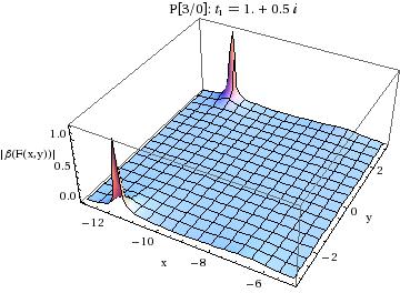
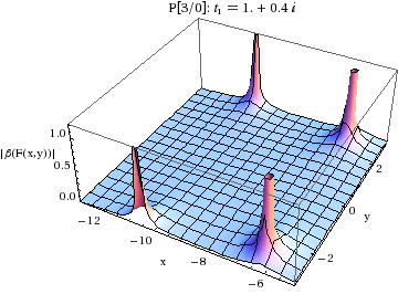
   Figure 12: (a) $|\beta(F(z))|$ as a function of $z=x+iy$ for the beta-function (21) with $f(Y)$ being cubic polynomial with $t_{1}=1+i0.5$ ($t_{2}=1-i0.5,t_{3}=-3.67591$); (b) the same as in (a), but with $t_{1}=1+i0.4$ ($t_{2}=1-i0.4,t_{3}=-3.98969$).

   This can be understood in the following way. The expression for the location of poles $z_{\rm p}$ is given by Eq. (55), with the sum there over $j=1,2,3$. Usually softwares such as MATHEMATICA give for logarithms $\ln U$ of complex arguments $U$ expressions with imaginary part $-\pi<{\rm Im}(\ln U)\leq\pi$. In this case, if only the term $\ln(-1)$ in Eq. (55) gets replaced by $[\ln(-1)-i2\pi]=-i\pi$, the resulting $z_{\rm p}$ has ${\rm Im}z_{\rm p}=-i\pi$, in both cases $t_{1}=1+i0.5$ and $t_{1}=1+i0.4$. Namely, $z_{\rm p}=-11.6312-i\pi$ and $z_{\rm p}=-10.5023-i\pi$, respectively. However, if we, in addition, replace $\ln[-t_{2}/(a_{0}/a_{\rm in}-t_{2})]$ by $\ln[-t_{2}/(a_{0}/a_{\rm in}-t_{2})]+i2\pi$, we get in the case of $t_{1}=1+i0.4$ a pole location $z_{\rm p}$ inside the physical stripe $-\pi\leq{\rm Im}z<\pi$: $z_{\rm p}=-6.32336-i2.6005$, which is the location of one of the Landau poles seen in Fig. 12(b); the other Landau pole is at $z_{\rm p}-6.32336+i2.6005$.

   In general, by adding to each of the logarithms of complex arguments in Eq. (55) multiples of $i2\pi$, we end up with a set of possible pole locations $z_{\rm p}$. Only those values which lie within the physical stripe $-\pi\leq{\rm Im}z<\pi$ are candidates for the location of (Landau) poles. However, in practice, only some of them represent poles $F(z_{\rm p})=\infty$, while others may have finite values of $F(z_{\rm p})$. This is so because the RGE integration, for the physical stripe of $z$’s, with a specific initial condition at $z=0$, will not cover all the possibilities of these multiples.

3. Yet another possibility is to have some roots $t_{j}$ real positive. Since we have $a_{0}\equiv a(Q^{2}=0)$ by our notation, the value $a=a_{0}$ is a root of the beta function $\beta(a)$, and there are no other roots of $\beta(a)$ in the positive interval $0<a<a_{0}$ [note that $\beta(0)=0$ by asymptotic freedom]. Therefore, we are not allowed to have $t_{j}>1$ since this would imply that $a_{j}=a_{0}/t_{j}<a_{0}$ is a root of $\beta(a)$; hence if $t_{j}$ is positive it must lie in the interval $0<t_{j}<1$. Such $t_{j}$’s then fulfill the relations $(0<t_{j}<1<a_{0}/a_{\rm in})$ and hence give a nonreal value of the logarithm $\ln(-t_{j}/(a_{0}/a_{\rm in}-t_{j}))$ in Eq. (55); the value of $B_{j}$ is real. Therefore, in such a case we generally obtain ${\rm Im}z_{\rm p}\not=-\pi$, i.e., we generally obtain a Landau pole.

4. We may obtain Landau poles, or Landau singularities, in several other cases, e.g., when some of the poles $u_{k}$ of the beta function are larger than unity. However, a systematic (semi-)analytic analysis of these problems appears to be too difficult here. We just mention, as an aside, that the appearance of Landau singularities [e.g., finite discontinuities of $F(z)$] usually implies the appearance of Landau poles [infinities of $F(z)$].

When $M\leq N-2$, the implicit solution of the type (52) obtains additional terms on the rhs: $\ln(F(z))$, $F(z)$, …, $F(z)^{N-M-2}$ (if $M\leq N-3$) [if $M=N-2$: only $\ln F(z)$]. In this case the poles $|F(z_{\rm p})|=\infty$ are reached at $z_{\rm p}=-\infty$, i.e., $Q^{2}=0$. This implies that in such cases the condition $a(Q^{2}=0)\equiv a_{0}<\infty$ cannot be fulfilled.

Appendix B Massless part of the strangeless tau decay ratio

At present, the most precisely measured low-energy observable referring to an inclusive process is the ratio $R_{\tau}(\Delta S=0)$, which is proportional to the branching ratio of $\tau$-decays into nonstrange hadrons. Consequently, it plays a central role for testing the validity of our anQCD approach. However, for a a careful comparison of the available experimental result with our theoretical prediction it is essential to extract from the quantity $R_{\tau}(\Delta S=0)$ the pure massless QCD-canonic part $r_{\tau}\equiv r_{\tau}(\Delta S=0,m_{q}=0)$. This analysis has already been presented in Appendix E of Ref. CV2 . Here we redo it, but with updated experimental values of $R_{\tau}(\Delta S=0)$, of the Cabibbo-Kobayashi-Maskawa (CKM) matrix element $|V_{ud}|$ and of higher-twist contributions. The strangeless (V+A)-decay ratio extracted from measurements by the ALEPH Collaboration ALEPH2 ; ALEPH3 and updated in Ref. DDHMZ is

$$R_{\tau}(\triangle S\!=\!0) \equiv \frac{\Gamma(\tau^{-}\to\nu_{\tau}{\rm hadrons}(\gamma))}{\Gamma(\tau^{-}\to\nu_{\tau}e^{-}{\overline{\nu}_{e}}(\gamma))}-R_{\tau}(\triangle S\!\not=\!0)$$ (57)

$$= 3.479\pm 0.011\ .$$ (58)

The canonic massless quantity $r_{\tau}(\triangle S=0,m_{q}=0)$ is obtained from the above quantity by removing the non-QCD [CKM and electroweak (EW)] factors and contributions, as well as chirality-violating (quark mass) contributions

$$r_{\tau}(\triangle S=0,m_{q}=0) = \frac{R_{\tau}(\triangle S=0)}{3|V_{ud}|^{2}(1+{\delta}_{{\rm EW}})}-(1+\delta_{\rm EW}^{\prime})-\delta r_{\tau}(\triangle S=0,m_{u,d}\not=0)\ .$$ (59)

This quantity is massless QCD-canonic, i.e., its pQCD expansion is $r_{\tau}(\triangle S=0,m_{q}=0)_{\rm pt}=a+{\cal O}(a^{2})$. The updated value of the CKM matrix element $|V_{ud}|$ is PDG2008

$$|V_{ud}|=0.97418\pm 0.00027\ .$$ (60)

The EW correction parameters are $1+\delta_{\rm EW}=1.0198\pm 0.0006$ ALEPH2 ; ALEPH3 and $\delta_{\rm EW}^{\prime}=0.0010$ Braaten:1990ef . The (V+A)-channel corrections $\delta r_{\tau}(\triangle S=0,m_{u,d}\not=0)$ due to the nonzero quark masses are Braaten:1988hc ; ALEPH3 the sum of corrections $(\delta_{ud,V}^{(D)}+\delta_{ud,A}^{(D)})/2$ with dimensions $D=2,4,6,$ and $8$. It appears that, among the chirality-nonviolating $D\geq 2$ contributions, the only possibly nonnegligible Ioffe is the $D=4$ contribution $\delta_{\langle GG\rangle}=(11/4)\alpha_{s}^{2}(m_{\tau}^{2})\langle aGG\rangle/m_{\tau}^{4}$ from gluon condensate. The authors of Ref. DDHMZ obtained from their fit the gluon condensate value $\langle aGG\rangle=(-1.5\pm 0.3)\times 10^{-2}\ {\rm GeV}^{4}$, giving thus $\delta_{\langle GG\rangle}\approx-5\times 10^{-4}$; their entire value of higher dimension contributions ($2\leq D\leq 8$) to $r_{\tau}(\triangle S=0,m_{u,d}\not=0)$ is $(-6.3\pm 1.4)\times 10^{-3}$. On the other hand, the value of the gluon condensate may be compatible with zero; e.g., the $\tau$-decay analysis of Ref. Ioffe based on sum rules gives $\langle aGG\rangle=(0.005\pm 0.004)\ {\rm GeV}^{4}$ which is almost compatible with zero. In our analysis we assume that this is the case, i.e., zero value of the gluon condensate. With this assumption, the higher dimension contributions to $r_{\tau}(\triangle S=0,m_{u,d}\not=0)$ are only the chirality-violating (i.e., due to nonzero quark mass) terms, their value being thus

$$\delta r_{\tau}(\triangle S=0,m_{u,d}\not=0)=(-5.8\pm 1.4)\times 10^{-3}\ .$$ (61)

Using the aforementioned results in Eq. (59) leads to

$$r_{\tau}(\triangle S=0,m_{q}=0)_{\rm exp.}=0.203\pm 0.004\ ,$$ (62)

where the experimental uncertainties were added in quadrature. The uncertainty here is dominated by the experimental uncertainty $\delta R_{\tau}=\pm 0.011$, Eq. (58). The central value (62) would increase to $0.204$ if the gluon condensate value $\langle aGG\rangle=(-1.5\pm 0.3)\times 10^{-2}\ {\rm GeV}^{4}$ of Ref. DDHMZ was taken. The central value $0.203$ of Eq. (62) is also obtained by using the analysis and results of Ref. Ioffe , but with the updated values $R_{\tau}(\triangle S\!=\!0)$ of Eq. (58) and $|V_{ud}|$ of Eq. (60).

Appendix C Higher order terms in analytic QCD

Here we summarize the general approach to calculate higher order corrections in analytic QCD (anQCD) models, as described first in our earlier works CV1 ; CV2 . In order not to confuse the general analytic coupling $a(Q^{2})$ with pQCD coupling $a_{\rm pt}(Q^{2})$, we will use in this Appendix the notation ${\mathcal{A}}_{1}(Q^{2})$ for the analytic coupling.

First we note that the analytic coupling ${\mathcal{A}}_{1}(Q^{2})$ does not fulfill the ITEP-OPE conditions (5) in any of the anQCD models that have appeared in the literature up to now. Nonfulfillment of ITEP-OPE conditions implies that the respective beta function $\beta({\mathcal{A}}_{1})\equiv\partial{\mathcal{A}}_{1}(Q^{2})/\partial\ln Q^{2}$ is not analytic in ${\mathcal{A}}_{1}$ (cf. arguments in Sec. II). Consequently, in these models the beta function, which is usually not known explicitly, cannot be Taylor expanded around ${\mathcal{A}}_{1}=0$, and therefore the powers ${\mathcal{A}}_{1}^{n}$ cannot be expected to be the analytized analogs of $a_{\rm pt}^{n}$. In fact, they usually are not. The construction of ${\mathcal{A}}_{n}(Q^{2})$, the analytic analogs of $a_{\rm pt}(Q^{2})^{n}$ ($n\geq 2$), is yet another important ingredient in anQCD.

A spacelike massless observable ${\cal D}(Q^{2})$, in its canonical form, has the following perturbation series:

$${\cal D}(Q^{2})_{\rm pt}=a_{\rm pt}+d_{1}a_{\rm pt}^{2}+d_{2}a_{\rm pt}^{3}+\cdots\ ,$$ (63)

and the corresponding truncated perturbation series (TPS) is

$${\cal D}(Q^{2})_{\rm pt}^{[N]}=a_{\rm pt}+d_{1}a_{\rm pt}^{2}+\cdots d_{N-1}a_{\rm pt}^{N}\ .$$ (64)

Here, $a_{\rm pt}$ and $d_{j}$’s have given renormalization scale (RScl) and scheme (RSch) dependences. Analytization means, in the first instance, to replace in the first term $a_{\rm pt}$ by ${\mathcal{A}}_{1}(Q^{2})$. For treating the higher order terms, there are, in principle, several options at hand. For instance, one could replace all powers of $a_{\rm pt}$ by the corresponding powers of ${\mathcal{A}}_{1}$ ($a_{\rm pt}^{n}\mapsto{\mathcal{A}}_{1}^{n}$). Or, as is done in MA, one could subject each $a_{\rm pt}^{n}$ to an analogous analytization procedure as ${\mathcal{A}}_{1}$ (if such an analogous procedure unambiguously exists), yielding additional analytic couplings $a_{\rm pt}^{n}\mapsto{\mathcal{A}}_{n}$, where, in general, ${\mathcal{A}}_{n}\not={\mathcal{A}}_{1}^{n}$. In MA such a prescription unambiguously exists. The advantage of such a prescription in MA lies in the fact that the RGEs governing the running of ${\mathcal{A}}_{n}^{\rm(MA)}$’s, as well as the RSch dependence of ${\mathcal{A}}_{n}^{\rm(MA)}$’s, are identical to the corresponding pQCD RGEs and RSch dependence once the replacements $a_{\rm pt}^{n}\mapsto{\mathcal{A}}_{n}^{\rm(MA)}$ are performed there Magradze . We consider this property as physically important, especially because there is a clear hierarchy ${\mathcal{A}}_{1}^{\rm(MA)}>|{\mathcal{A}}_{2}^{\rm(MA)}|>|{\mathcal{A}}_{3}^{\rm(MA)}|\cdots$ at all positive $Q^{2}$ values. Among other things, this hierarchy implies that the MA-analytized version of the TPS Eq. (64)

$${\cal D}(Q^{2})_{\rm(MA)}^{[N]}={\mathcal{A}}_{1}^{\rm(MA)}+d_{1}{\mathcal{A}}_{2}^{\rm(MA)}+\cdots d_{N-1}{\mathcal{A}}_{N}^{\rm(MA)}\ ,$$ (65)

becomes systematically more RScl and RSch independent when the truncation index $N$ increases

$$\frac{\partial{\cal D}(Q^{2};{\rm RS})_{\rm(MA)}^{[N]}}{\partial({\rm RS})}=k_{N}{\mathcal{A}}_{N+1}^{\rm(MA)}+{\cal O}({\mathcal{A}}_{N+2}^{\rm(MA)})\ .$$ (66)

Here, “RS” stands for logarithm $\ln\mu^{2}$ of RScl $\mu$, or for any RSch parameter $c_{j}=\beta_{j}/\beta_{0}$ ($j\geq 2$).

However, when constructing anQCD models beyond MA, by changing the discontinuity function $\rho_{1}(\sigma)={\rm Im}a_{\rm pt}(-\sigma-i\epsilon)$ appearing in the dispersion relation (6) for ${\mathcal{A}}_{1}^{\rm(MA)}(Q^{2})$ Nesterenko2 ; CV1 ; CV2 , or by different constructions of ${\mathcal{A}}_{1}(Q^{2})$ (cf. Webber:1998um ; Srivastava:2001ts ; Simonov ; Nesterenko ; Alekseev:2005he and references therein), the meaning of “analogous analytization” of higher powers $a_{\rm pt}^{n}$ becomes unclear or, at best, ambiguous. On the other hand, it is almost imperative to maintain relations (66) in any anQCD model with hierarchy ${\mathcal{A}}_{1}>|{\mathcal{A}}_{2}|>|{\mathcal{A}}_{3}|\cdots$, because then the physical condition of RScl and RSch independence of the evaluated observables is guaranteed to be increasingly well fulfilled at any $Q^{2}$ when the number of terms increases.

Furthermore, it is preferable to have the higher power analogs $a_{\rm pt}^{n}\mapsto{\mathcal{A}}_{n}$ not simply constructed as ${\mathcal{A}}_{n}\equiv({\mathcal{A}}_{1})^{n}$, but rather by application of linear (in ${\mathcal{A}}_{1}$) operations on ${\mathcal{A}}_{1}$, such as, e.g., derivatives and linear combinations thereof. The underlying reason is the compatibility with linear integral transformations (such as Fourier and Laplace) Shirkov:1999np . In linear transformations, the image of a power of a function is not the power of the image of the function.

The construction of higher order analogs ${\mathcal{A}}_{n}$ (applicable to any anQCD model) which obey all these conditions was first presented in Refs. CV1 ; CV2 . The procedure proposed there for obtaining ${\mathcal{A}}_{n}$ from a given anQCD coupling ${\mathcal{A}}_{1}$, in a given RSch, is the following: First we define the logarithmic derivatives of ${\mathcal{A}}_{1}(\mu^{2})$ (where $\mu^{2}=\kappa Q^{2}$ is any chosen RScl), i.e., we define

$${\widetilde{\mathcal{A}}}_{n+1}(\mu^{2})\left(\equiv{\widetilde{a}}_{n+1}(\mu^{2})\right)=\frac{(-1)^{n}}{\beta_{0}^{n}n!}\frac{\partial^{n}{\mathcal{A}}_{1}(\mu^{2})}{\partial(\ln\mu^{2})^{n}}\ ,\qquad(n=1,2,\ldots)\ .$$ (67)

In order to understand the following construction of ${\mathcal{A}}_{n}$’s given below, it is convenient to consider first the corresponding logarithmic derivatives in pQCD

$${\widetilde{a}}_{{\rm pt},n+1}(\mu^{2})\equiv\frac{(-1)^{n}}{\beta_{0}^{n}n!}\frac{\partial^{n}a_{\rm pt}(\mu^{2})}{\partial(\ln\mu^{2})^{n}}\ .\qquad(n=1,2,\ldots)$$ (68)

These are related to the powers $a_{\rm pt}^{n}$ via relations involving the $c_{j}$ coefficients of the pQCD RGE Eq. (4)

$${\widetilde{a}}_{{\rm pt},2} = a_{\rm pt}^{2}+c_{1}a_{\rm pt}^{3}+c_{2}a_{\rm pt}^{4}+\cdots\ ,$$ (69)

$${\widetilde{a}}_{{\rm pt},3} = a_{\rm pt}^{3}+\frac{5}{2}c_{1}a_{\rm pt}^{4}+\cdots\ ,$$ (70)

$${\widetilde{a}}_{{\rm pt},4} = a_{\rm pt}^{4}+\cdots\ ,\qquad{\rm etc.}$$ (71)

The above relations are obtained by (repeatedly) applying the pQCD RGE. The inverse relations are

$$a_{\rm pt}^{2} = {\widetilde{a}}_{{\rm pt},2}-c_{1}{\widetilde{a}}_{{\rm pt},3}+\left(\frac{5}{2}c_{1}^{2}-c_{2}\right){\tilde{a}}_{{\rm pt},4}+\cdots\ ,$$ (72)

$$a_{\rm pt}^{3} = {\widetilde{a}}_{{\rm pt},3}-\frac{5}{2}c_{1}{\widetilde{a}}_{{\rm pt},4}+\cdots\ ,$$ (73)

$$a_{\rm pt}^{4} = {\widetilde{a}}_{{\rm pt},4}+\cdots\ ,\qquad{\rm etc.}$$ (74)

Now we adopt the following replacement on the rhs of Eqs. (72)-(74):

$$a_{\rm pt}\mapsto{\mathcal{A}}_{1}\ ,\quad{\widetilde{a}}_{{\rm pt},n+1}\mapsto{\widetilde{\mathcal{A}}}_{n+1}\quad(n=1,2,\ldots)\ ,$$ (75)

and use the generated expressions as definitions of ${\mathcal{A}}_{n}$, the higher power analogs of pQCD powers $a_{\rm pt}^{n}$

$${\mathcal{A}}_{2} = {\widetilde{\mathcal{A}}}_{2}-c_{1}{\widetilde{\mathcal{A}}}_{3}+\left(\frac{5}{2}c_{1}^{2}-c_{2}\right){\widetilde{\mathcal{A}}}_{4}+\cdots\ ,$$ (76)

$${\mathcal{A}}_{3} = {\widetilde{\mathcal{A}}}_{3}-\frac{5}{2}c_{1}{\widetilde{\mathcal{A}}}_{4}+\cdots\ ,$$ (77)

$${\mathcal{A}}_{4} = {\widetilde{\mathcal{A}}}_{4}+\cdots\ ,\qquad{\rm etc.}$$ (78)

It is then straightforward to see that the analytic (“an”) series obtained from the perturbation series (63) via replacements $a_{\rm pt}\mapsto{\mathcal{A}}_{1}$, $a_{\rm pt}^{n}\mapsto{\mathcal{A}}_{n}$

$${\cal D}(Q^{2})_{\rm an}={\mathcal{A}}_{1}+d_{1}{\mathcal{A}}_{2}+d_{2}{\mathcal{A}}_{3}+\cdots\ ,$$ (79)

gives the corresponding truncated analytic series

$${\cal D}(Q^{2})_{\rm an}^{[N]}={\mathcal{A}}_{1}+d_{1}{\mathcal{A}}_{2}+\cdots d_{N-1}{\mathcal{A}}_{N}\ ,$$ (80)

which really fulfills the condition (66) of increasingly good RS-independence, now in any anQCD model

$$\frac{\partial{\cal D}(Q^{2};{\rm RS})_{\rm an}^{[N]}}{\partial({\rm RS})}=k_{N}{\mathcal{A}}_{N+1}+{\cal O}(A_{N+2})\ ,\qquad({\rm RS}=\ln\mu^{2};c_{2};c_{3};\ldots)\ .$$ (81)

This relation continues to hold even if we truncate relations (76)-(78) at the order $\sim{\mathcal{A}}_{N}$ (including the latter).

The above presentation suggests that, instead of the perturbation series (63) in powers of $a_{\rm pt}$, a modified perturbation series in logarithmic derivatives ${\widetilde{a}}_{\rm pt,n+1}$ (68) can be used

$${\cal D}(Q^{2})_{\rm mpt}=a_{\rm pt}+{\widetilde{d}}_{1}{\widetilde{a}}_{{\rm pt},2}+{\widetilde{d}}_{2}{\widetilde{a}}_{{\rm pt},3}+\cdots\ ,$$ (82)

whose truncated form is

$${\cal D}(Q^{2})_{\rm mpt}^{[N]}=a_{\rm pt}+{\widetilde{d}}_{1}{\widetilde{a}}_{{\rm pt},2}+\cdots{\widetilde{d}}_{N-1}{\widetilde{a}}_{{\rm pt},N}\ ,$$ (83)

where “m” in the subscript stands for “modified,” and the modified coefficients ${\widetilde{d}}_{j}$ ($j=1,\ldots,N-1$) are related to the original coefficients $d_{j}$

$${\widetilde{d}}_{1} = d_{1}\ ,$$ (84)

$${\widetilde{d}}_{2} = d_{2}-c_{1}d_{1}\ ,$$ (85)

$${\widetilde{d}}_{3} = d_{3}-\frac{5}{2}c_{1}d_{2}+\left(\frac{5}{2}c_{1}^{2}-c_{2}\right)d_{1}\ ,\qquad{\rm etc.}$$ (86)

When applying analytization to the modified perturbation series (82), via replacements (75), we obtain modified analytic series (“man”)

$${\cal D}(Q^{2})_{\rm man}={\mathcal{A}}_{1}+{\widetilde{d}}_{1}{\widetilde{\mathcal{A}}}_{2}+{\widetilde{d}}_{2}{\widetilde{\mathcal{A}}}_{3}+\cdots\ ,$$ (87)

whose truncated version is

$${\cal D}(Q^{2})_{\rm man}^{[N]}={\mathcal{A}}_{1}+{\widetilde{d}}_{1}{\widetilde{\mathcal{A}}}_{2}+\cdots{\widetilde{d}}_{N-1}{\widetilde{\mathcal{A}}}_{N}\ .$$ (88)

Its RS dependence is

$$\frac{\partial{\cal D}(Q^{2};{\rm RS})_{\rm man}^{[N]}}{\partial({\rm RS})}={\widetilde{k}}_{N}{\widetilde{\mathcal{A}}}_{N+1}+{\cal O}({\widetilde{\mathcal{A}}}_{N+2})\quad(\sim{\mathcal{A}}_{N+1})\ ,\qquad({\rm RS}=\ln\mu^{2};c_{2};c_{3};\ldots)\ .$$ (89)

It is interesting that in virtually all anQCD models [i.e., models that define ${\mathcal{A}}_{1}(Q^{2})$] holds the hierarchy ${\mathcal{A}}_{1}>|{\widetilde{\mathcal{A}}}_{2}|>|{\widetilde{\mathcal{A}}}_{3}|>\cdots$ at (almost) all complex $Q^{2}$. Therefore, Eq. (89) signals an increasingly weak RS dependence of ${\cal D}(Q^{2})_{\rm man}^{[N]}$ when $N$ increases, at any value of $Q^{2}$ and RScl $\mu^{2}$.

We stress that the analytic (“an”) and modified analytic (“man”) series [Eqs. (79) and (87), respectively], if they converge, are identical to each other due to relations (84)-(86) and (76)-(78).

In the specific case of MA, i.e., when ${\mathcal{A}}_{1}={\mathcal{A}}_{1}^{\rm(MA)}$ of Ref. ShS , it can be shown (using the results of Ref. Magradze ) that the above procedure, Eqs. (76)-(78), gives the same higher power analogs ${\mathcal{A}}_{n}^{\rm(MA)}$ as the analytization procedure of Ref. MSS (APT) that uses the MA-type dispersion relation involving ${\rm Im}a_{\rm pt}^{n}(Q^{2}=-\sigma-i\epsilon)$

$${\mathcal{A}}_{n}^{\rm(MA)}(Q^{2})=\frac{1}{\pi}\int_{0}^{\infty}\;d\sigma\frac{\rho_{n}^{\rm(pt)}(\sigma)}{\sigma+Q^{2}}\ ,$$ (90)

where $\rho_{n}^{\rm(pt)}(\sigma)={\rm Im}a_{\rm pt}^{n}(-\sigma-i\epsilon)$ ($n=2,\ldots$). We note that ${\mathcal{A}}_{n}^{\rm(MA)}\not=({\mathcal{A}}_{1}^{\rm(MA)})^{n}$. Furthermore, construction of ${\mathcal{A}}_{n}$ according to relations (76)-(78) in other models of anQCD (e.g., where ${\mathcal{A}}_{1}$ is constructed from a modified $\rho_{1}\not=\rho_{1}^{\rm(pt)}$, e.g. Refs. Nesterenko2 ; CV1 ; CV2 ) also in general leads to ${\mathcal{A}}_{n}\not={\mathcal{A}}_{1}^{n}$. However, if analytic $A_{1}(Q^{2})\equiv a(Q^{2})$ is constructed from RGE with beta function $\beta(a)$ analytic at $a=0$, as is the case in the present work and Ref. CKV1 , it is straightforward to see that construction (76)-(78) gives

$${\mathcal{A}}_{n}=a^{n}\quad(n=1,2,\ldots)\ .$$ (91)

In those anQCD models of analytic ${\mathcal{A}}_{1}(Q^{2})$ where the aforedescribed construction gives ${\mathcal{A}}_{n}\not={\mathcal{A}}_{1}^{n}$ for $n\geq 2$ (such models do not appear in the present work), using ${\mathcal{A}}_{1}^{n}$ instead of ${\mathcal{A}}_{n}$ is not a good idea for at least two reasons: (1) such a construction is formally not linear in ${\mathcal{A}}_{1}$ [see the discussion before Eq. (67)]; (2) the RS dependence of the resulting truncated “power” analytic series

$${\cal D}_{\rm pan}(Q^{2})^{[N]}={\mathcal{A}}_{1}+d_{1}{\mathcal{A}}_{1}^{2}+\cdots d_{N-1}{\mathcal{A}}_{1}^{N}$$ (92)

is not entirely analogous to Eq. (81) or Eq. (89), but is rather

$$\frac{\partial{\cal D}(Q^{2};{\rm RS})_{\rm pan}^{[N]}}{\partial({\rm RS})}=k_{N}{\mathcal{A}}_{1}^{N+1}+{\cal O}({\mathcal{A}}_{1}^{N+2})+{\rm NP}_{(N)}\ ,$$ (93)

where ${\rm NP}_{(N)}$ is an increasingly complicated expression of nonperturbative terms (such as $1/Q^{2n}$) when $N$ increases, and $|{\rm NP}_{(N)}|$ in general does not decrease when $N$ increases.

Appendix D Leading-$\beta_{0}$ (skeleton-motivated) resummation in anQCD

First we summarize here the resummation formalism for the leading-$\beta_{0}$ (LB) part of inclusive spacelike QCD observables in anQCD models, as presented in CV1 ; CV2 . Subsequently, we present application of this formalism to LB resummation for the Bjorken polarized sum rule (BjPSR) $d_{\rm Bj}(Q^{2})$ and, in a newly modified form, to the $\tau$ decay ratio $r_{\tau}$.

Massless spacelike QCD observables ${\cal D}(Q^{2})$, in canonical form, have the pQCD (“pt”) expansion (63) in powers of $a_{\rm pt}$, where $a_{\rm pt}=a_{\rm pt}(\mu^{2};c_{2},\ldots)$ is defined at a given RScl $\mu$ and in a given RSch ($c_{2},c_{3},\dots$). In the scaling definition of $\mu$ we use the convention $\Lambda={\overline{\Lambda}}$, which is the ${\overline{\rm MS}}$ reference scale for RScl’s $\mu$ [the so-called $V$ scheme $\Lambda_{V}$ is related to ${\overline{\Lambda}}$ via ${\overline{\Lambda}}^{2}=\Lambda_{V}^{2}\exp({\overline{\cal C}})$, where ${\overline{\cal C}}=-5/3$]. The considered RSch classes will be such that the RSch coefficients $\beta_{k}\equiv\beta_{0}c_{k}$ ($k\geq 2$) are polynomials in $n_{f}$, and consequently in $\beta_{0}=(11-2n_{f}/3)/4$

$$\beta_{k}\equiv\beta_{0}c_{k}=\sum_{j=0}^{k}b_{kj}\beta_{0}^{j},\qquad(k=2,3,\ldots)$$ (94)

We recall that $\beta_{0}=(11-2n_{f}/3)/4$ and $\beta_{1}=(102-38n_{f}/3)/16$ are both universal (RSch-independent) parameters. RSch’s ${\overline{\rm MS}}$ and ’t Hooft are clearly special cases of such RSch’s. The RSch independence of ${\cal D}(Q^{2})$ implies a specific dependence of coefficients $d_{n}$ on the RSch parameters Stevenson ; this and relations (94) imply that the coefficients $d_{n}$ have specific expansions in powers of $\beta_{0}$

$$d_{1}=c^{(1)}_{11}\beta_{0}+c^{(1)}_{10},\qquad d_{n}=\sum_{k=-1}^{n}c^{(1)}_{nk}\beta_{0}^{k}\ .$$ (95)

We note that $c^{(1)}_{1,-1}=0$. In ${\overline{\rm MS}}$ RSch, the negative power term $\propto 1/\beta_{0}$ does not appear. Relations (95) and (84)-(86) imply that the modified perturbation (“mpt”) expansion (82) of ${\cal D}(Q^{2})$ in logarithmic derivatives ${\widetilde{a}}_{\rm pt,n+1}$ of Eq. (68) have coefficients ${\widetilde{d}}_{n}$ of a form similar to (95)

$${\widetilde{d}}_{n}=\sum_{k=-1}^{n}{\widetilde{c}}^{(1)}_{nk}\beta_{0}^{k}\ .$$ (96)

Specifically, the leading-$\beta_{0}$ terms in Eqs. (95) and (96) coincide

$${\widetilde{c}}^{(1)}_{nn}=c^{(1)}_{nn}$$ (97)

The LB resummation of the inclusive spacelike ${\cal D}(Q^{2})$ is obtained in pQCD via integration of $a_{\rm pt}(\mu^{2})$ over various scales $\mu^{2}=tQ^{2}\exp({\overline{\cal C}})$ and weighted with a characteristic function $F_{\cal D}^{\cal{E}}(t)$ according to formalism of Ref. Neubert

$${\cal D}^{\rm(LB)}_{\rm pt}(Q^{2})\equiv\int_{0}^{\infty}\frac{dt}{t}\>F_{\cal D}^{\cal{E}}(t)\>a_{\rm pt}(tQ^{2}e^{\overline{\cal C}})\ .$$ (98)

The integration cannot be performed unambiguously, due to the Landau poles of $a_{\rm pt}$ at low values of $t$. In anQCD $a_{\rm pt}$ here is simply replaced by analytic ${\mathcal{A}}_{1}$ ($\equiv a$)

$${\cal D}^{\rm(LB)}_{\rm an}(Q^{2})\equiv\int_{0}^{\infty}\frac{dt}{t}\>F_{\cal D}^{\cal{E}}(t)\>{\mathcal{A}}_{1}(tQ^{2}e^{\overline{\cal C}})\ ,$$ (99)

where now the integration is unambiguous since there are no Landau poles. Expansion of the analytic coupling ${\mathcal{A}}_{1}(tQ^{2}e^{\overline{\cal C}})$ around the RScl scale $\mu^{2}$, i.e., Taylor expansion in powers of ${\cal L}=\ln[\mu^{2}/(tQ^{2}e^{\overline{\cal C}})]$, gives

$${\cal D}^{\rm(LB)}_{\rm an}(Q^{2})={\mathcal{A}}_{1}+\sum_{n=1}^{\infty}c^{(1)}_{nn}\beta_{0}^{n}{\widetilde{\mathcal{A}}}_{n+1}\ .$$ (100)

We thus see that integral (99), in anQCD, represents exactly the leading-$\beta_{0}$ (LB) part of the modified analytic (“man”) expansion (87) in Appendix C. The truncated series of the latter is given in Eq. (88). We stress that the above expansion is performed at a given RScl $\mu$ and in a given RSch [$c_{2},c_{3},\ldots$ – cf. Eq. (94)]. In anQCD it is convenient to perform explicitly the LB resummation (99) since the integral there is finite, unambiguous, and RScl independent.

The characteristic function $F_{\cal D}^{\cal{E}}(t)$ for the BjPSR ${\cal D}(Q^{2})=d_{\rm Bj}(Q^{2})$ was calculated and used in Ref. CV1 (on the basis of the known Broadhurst:1993ru coefficients $c^{(1)}_{nn}$ for it), and was presented in Ref. CV2

$$F_{\rm Bj}(t)=\left\{\begin{array}[]{ll}(8/9)t\left[1-(5/8)t\right]&t\leq 1\\ (4/(9t))\left[1-1/(4t)\right]&t\geq 1\end{array}\right\}\ .$$ (103)

The (nonstrange massless) canonical semihadronic $\tau$ decay ratio $r_{\tau}\equiv r_{\tau}(\Delta S=0,m_{q}=0)$ is a timelike quantity, and can be expressed in terms of the massless current-current correlation function (V-V or A-A, both equal since massless) Tsai:1971vv

$$r_{\tau}=\frac{2}{\pi}\int_{0}^{m^{2}_{\tau}}\ \frac{ds}{m^{2}_{\tau}}\left(1-\frac{s}{m^{2}_{\tau}}\right)^{2}\left(1+2\frac{s}{m^{2}_{\tau}}\right){\rm Im}\Pi(Q^{2}=-s)\ .$$ (104)

Use of the Cauchy theorem in the $Q^{2}$ plane and then integration by parts leads to the following contour integral form Braaten:1988hc ; Beneke:2008ad :

$$r_{\tau}=\frac{1}{2\pi}\int_{-\pi}^{+\pi}d\phi\ (1+e^{i\phi})^{3}(1-e^{i\phi})\ d_{\rm Adl}(Q^{2}=m_{\tau}^{2}e^{i\phi})\ ,$$ (105)

with $d_{\rm Adl}(Q^{2})=-d\Pi(Q^{2})/d\ln Q^{2}$ being the massless Adler function. In pQCD, use of the Cauchy theorem to the expression (104) is formally not allowed. This is so because $\Pi_{\rm pt}(Q^{2})$, being a power series in $a_{\rm pt}(Q^{2})$ [or: $a_{\rm pt}(\kappa Q^{2})$], has Landau singularities along the positive axis $0<Q^{2}\leq\Lambda^{2}$. In pQCD, expressions (104) and (105) are two different quantities; in anQCD models they are always the same.

The massless Adler function $d_{\rm Adl}(Q^{2})$ is a spacelike (quasi)observable. On the basis of the known coefficients $c^{(1)}_{nn}$ for it Broadhurst ; Beneke , its characteristic function $F_{\rm Adl}(\tau)$ was obtained in Ref. Neubert , and from it and using relation (105) the characteristic function for $r_{\tau}$ was obtained in Ref. Neubert2 , in the timelike LB form

$$r_{\tau}(\Delta S=0,m_{q}=0)^{\rm(LB)}=\int_{0}^{\infty}\frac{dt}{t}\>F_{r}^{\cal{M}}(t)\>{\mathfrak{A}}_{1}(te^{\cal C}m_{\tau}^{2})\ .$$ (106)

Here, the superscript ${\cal{M}}$ indicates that these are Minkowskian (timelike) quantities; ${\mathfrak{A}}_{1}$ is the timelike coupling

$${\mathfrak{A}}_{1}(s) = \frac{1}{\pi}\int_{s}^{\infty}\frac{d\sigma}{\sigma}{\rho}_{1}(\sigma)\ ;$$ (107)

and the characteristic function $F_{r}^{\cal{M}}(t)$ was obtained in Neubert2 .

It turns out that, in the calculations in the present work, it is inconvenient to calculate the LB-contribution to $r_{\tau}$ by using formula (106) which involves function ${\mathfrak{A}}_{1}(s)$. This inconvenience consists in the following: in this work, RGE (15) [$\Leftrightarrow$ Eqs. (16)-(17)] is integrated in the entire physical stripe in the complex $z$ plane, and as a result of this we numerically obtain, among other things, the quantity $\rho_{1}(\sigma)={\rm Im}a(Q^{2}=-\sigma-i\epsilon)={\rm Im}F(z=|z|-i\pi)$ [with: $|z|=\ln(\sigma/\mu_{\rm in}^{2})$]; to obtain the quantity ${\mathfrak{A}}_{1}(s)$, yet another numerical integration (107) is needed, and then we go with this ${\mathfrak{A}}_{1}(s)$ into the integration (106). There are too many successive numerical integrations involved, and the precision of calculation is expected to be low.

Therefore, we perform in integral (106) integration by parts, using relation $d{\mathfrak{A}}_{1}(s)/d\ln s=-\rho_{1}(s)/\pi$ [cf. Eq. (107)], and we obtain the expression of $r_{\tau}^{\rm(LB)}$ in terms of the discontinuity function $\rho_{1}(s)$:

$$r_{\tau}^{\rm(LB)}=\frac{1}{\pi}\int_{0}^{\infty}\frac{dt}{t}\>{\widetilde{F}}_{r}(t)\>\rho_{1}(te^{\cal{\overline{C}}}m_{\tau}^{2})\ ,$$ (108)

where

$${\widetilde{F}}_{r}(t)=\int_{0}^{t}\frac{dt^{\prime}}{t^{\prime}}\>F_{r}^{\cal{M}}(t^{\prime})\ .$$ (109)

Integration in (109) can be performed analytically, and the result for ${\widetilde{F}}_{r}(t)$ is ($C_{F}=4/3$):

$${\widetilde{F}}_{r}(t)/(4C_{F}) = -\frac{1}{12}\text{Li}_{2}(-t)\left(t^{4}+6t^{3}+18t^{2}+10t-12t\ln(t)-3\right)-2t\text{Li}_{3}(-t)$$ (110)

$$+\frac{1}{1728}{\Big{\{}}-72\ln(t)\left[t\left(-2t^{2}-47t+6\right)+2\left(t^{4}+6t^{3}+18t^{2}+10t-3\right)\ln(t+1)\right]$$

$$-259t^{4}-600t^{3}-6948t^{2}-5184t\zeta(3)+7344t+72(t+6)t^{3}\ln^{2}(t){\Big{\}}}\quad(t\leq 1),$$

$${\widetilde{F}}_{r}(t)/(4C_{F}) = \frac{1}{432}{\bigg{\{}}-36t(t^{3}+6t^{2}+18t-2)\text{Li}_{2}\left(-\frac{1}{t}\right)-108\text{Li}_{2}(-t)+864t\text{Li}_{3}\left(-\frac{1}{t}\right)$$ (111)

$$+432t\text{Li}_{2}\left(-\frac{1}{t}\right)(\ln(t)-1)-9\left[(t^{2}+8t+36)t^{2}+96\right]\ln(t+1)-t\left[9t(4t+23)+598\right]$$

$$-18\left[2t(t^{3}+6t^{2}+18t+22)-3\right]\ln^{2}(t)$$

$$+3\left[(3t^{4}+12t^{3}+42t^{2}-184t+111)+12(t^{2}+4t+9)(t+1)^{2}\ln(t+1)\right]\ln(t)$$

$$+9t(t^{3}+8t^{2}+36t-96)\ln\left(\frac{1}{t}+1\right)$$

$$+432(\ln(t)-2)\left[t\ln(t)-(t+1)\ln(t+1)\right]+648\zeta(3)-114\pi^{2}+841{\bigg{\}}}$$

$$-\frac{3\zeta(3)}{2}+\frac{2\pi^{2}}{9}-\frac{463}{1728}\quad(t\geq 1).$$

The function ${\widetilde{F}}_{r}(t)$ is continuous and monotonously increases when $t$ increases. Its value is zero at $t=0$, and one at $t=+\infty$. It is depicted in Figs. 13 as a function of $t$ and $\ln t$.

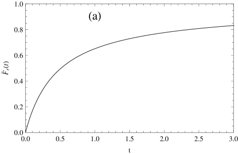
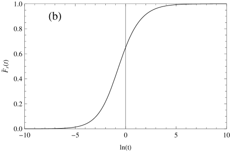
Figure 13: Characteristic function ${\widetilde{F}}_{r}(t)$ which appears in the LB integral (108) of $r_{\tau}$: (a) as a function of $t$; (b) as a function of $\ln t$.

Appendix E Inclusion of beyond-the-leading-$\beta_{0}$ (bLB) terms in anQCD

In pQCD, perturbation expansion of any massless spacelike observable ${\cal D}(Q^{2})$ can be written in the form (63) or (82). In the considered (large) RSch classes (94), the coefficients $d_{n}$ and ${\widetilde{d}}_{n}$ can be written in the form (95) and (96), respectively. Leading-$\beta_{0}$ (LB) resummation (99) reproduces one part of these terms, Eq. (100). In practice, for inclusive spacelike observables only the leading-$\beta_{0}$ parts $c^{(1)}_{nn}\beta_{0}^{n}$ of coefficients $d_{n}$ and ${\widetilde{d}}_{n}$ are known for all $n$ [cf. also Eq. (97)], while the coefficients known in their entirety are only the first two or three: $d_{1},d_{2},d_{3}$ [$\Leftrightarrow\ {\widetilde{d}}_{1},{\widetilde{d}}_{2},{\widetilde{d}}_{3}$, cf. Eqs. (84)-(86)]. For this reason, the most that one can include in the evaluation of any such observable in anQCD are all the LB contributions, Eq. (100), and the beyond-the-leading-$\beta_{0}$ (bLB) terms of order $a^{2},a^{3},$ and$a^{4}$ ($\Leftrightarrow$ of order ${\widetilde{a}}_{2},{\widetilde{a}}_{3},{\widetilde{a}}_{4}$].

In practice, the coefficients $d_{1},d_{2},d_{3}$ and $c^{(1)}_{nn}\beta_{0}^{n}$ are calculated and given in the literature in the ${\overline{\rm MS}}$ RSch [$c_{2}({\overline{\rm MS}}),c_{3}({\overline{\rm MS}}),\ldots$] and with RScl $\mu^{2}=Q^{2}$; we will denote such quantities with the bar over them. In general, the evaluations are performed in another RSch ($c_{2},c_{3},\ldots$) (e.g., in the present work the RSch as dictated by the chosen $\beta$ function used), and another RScl

$$\mu^{2}=Q^{2}\exp({\cal C})\qquad({\cal C}\sim 1)\ .$$ (112)

The LB contribution (99) is RScl independent; however, it depends on the RSch. The truncated bLB contribution still has some remnant RScl dependence due to truncation, and is RSch dependent.

The dependence of the coefficients ${\widetilde{d}}_{j}$ on RScl and RSch can be deduced systematically, by the requirement of RScl and RSch independence of the observable ${\cal D}$ and using the known RScl and RSch dependence of the pQCD coupling $a_{\rm pt}({\cal C};c_{2},c_{3},\ldots)$ Stevenson . The resulting dependence of ${\widetilde{d}}_{j}$ is

$${\widetilde{d}}_{1} = {\overline{\widetilde{d}}}_{1}+\beta_{0}{\cal C}\quad(=d_{1})\ ,$$ (113)

$${\widetilde{d}}_{2} = {\overline{\widetilde{d}}}_{2}+\left[2\beta_{0}{\cal C}{\overline{\widetilde{d}}}_{1}+\beta_{0}^{2}{\cal C}^{2}\right]-(c_{2}-{\overline{c}}_{2})\ ,$$ (114)

$${\widetilde{d}}_{3} = {\overline{\widetilde{d}}}_{3}+\left[3\beta_{0}{\cal C}{\overline{\widetilde{d}}}_{2}+3\beta_{0}^{2}{\cal C}^{2}{\overline{\widetilde{d}}}_{1}+\beta_{0}^{3}{\cal C}^{3}\right]+\left[-3({\overline{\widetilde{d}}}_{1}+\beta_{0}{\cal C})+\frac{5}{2}c_{1}\right](c_{2}-{\overline{c}}_{2})-\frac{1}{2}(c_{3}-{\overline{c}}_{3})\ ,$$ (115)

etc. On the other hand, the RScl independence of LB contribution (99)-(100) implies for the LB coefficients (97) the following RScl dependence (they are RSch independent)

$$c^{(1)}_{nn}=\sum_{k=0}^{n}\left(\begin{array}[]{c}n\\ k\end{array}\right){\overline{c}}^{(1)}_{kk}{\cal C}^{n-k}\ ,$$ (116)

where ${\overline{c}}^{(1)}_{00}=1$ by definition. When we subtract from the modified analytic (“man”) series (87) the LB contribution (100), we obtain the bLB contribution separately

$${\cal D}_{\rm man}^{\rm(LB+bLB)}(Q^{2}) = {\cal D}^{\rm(LB)}_{\rm an}(Q^{2})+{\cal D}^{\rm(bLB)}_{\rm man}(Q^{2})$$ (117)

$$= \int_{0}^{\infty}\frac{dt}{t}\>F_{\cal D}^{\cal{E}}(t)\>{\mathcal{A}}_{1}(tQ^{2}e^{\overline{\cal C}})+\sum_{n=1}^{\infty}(T_{\cal D})_{n}{\widetilde{\mathcal{A}}}_{n+1}\ ,$$

where ${\overline{\cal C}}=-5/3$ as mentioned earlier in Appendix D, ${\widetilde{\mathcal{A}}}_{n+1}$ are in RSch ($c_{2},c_{3},\ldots$) and at RScl $\mu^{2}=Q^{2}\exp({\cal C})$, and the coefficients $(T_{\cal D})_{n}$ are

$$(T_{\cal D})_{n}={\widetilde{d}}_{n}-c^{(1)}_{nn}\beta_{0}^{n}\ ,$$ (118)

where ${\widetilde{d}}_{n}$ and $c^{(1)}_{nn}$ are related with the corresponding (bar) quantities in ${\overline{\rm MS}}$ RSch and RScl $\mu^{2}=Q^{2}$ via relations (113)-(115) and (116). This, and application of relations (84)-(86) in ${\overline{\rm MS}}$ RSch and RScl $\mu^{2}=Q^{2}$, allows us to obtain the first three coefficients $(T_{\cal D})_{n}$ by knowing the first three coefficients ${\overline{d}}_{n}$ ($n=1,2,3$) (all ${\overline{c}}^{(1)}_{kk}$ are known).

Another variant of evaluation of ${\cal D}$ in anQCD is not to perform the LB resummation (99) in (117), but rather use its expanded form (100). This leads to

$${\cal D}_{\rm man}(Q^{2}) = {\mathcal{A}}_{1}+\sum_{n=1}^{\infty}{\widetilde{d}}_{n}{\widetilde{\mathcal{A}}}_{n+1}\ ,$$ (119)

where $a\equiv{\mathcal{A}}_{1}\equiv{\mathcal{A}}_{1}(Q^{2}\exp({\cal C});c_{2},\ldots)$. Series (119) was obtained in Appendix C in Eq. (87).

In principle, both series (117) and (119) must lead to the same result if the series are convergent. However, in practice, only the first three terms in the sums there ($n=1,2,3$) are known. Hence the series (117) and (119) truncated at $n=3$

$${\cal D}_{\rm man}^{\rm(LB+bLB)}(Q^{2})^{[4]} = \int_{0}^{\infty}\frac{dt}{t}\>F_{\cal D}^{\cal{E}}(t)\>{\mathcal{A}}_{1}(tQ^{2}e^{\overline{\cal C}})+\sum_{n=1}^{3}(T_{\cal D})_{n}{\widetilde{\mathcal{A}}}_{n+1}\ ,$$ (120)

$${\cal D}_{\rm man}(Q^{2})^{[4]} = {\mathcal{A}}_{1}+\sum_{n=1}^{3}{\widetilde{d}}_{n}{\widetilde{\mathcal{A}}}_{n+1}\ ,$$ (121)

will give in general somewhat different results, the difference being $\sim{\widetilde{\mathcal{A}}}_{5}(\sim{\mathcal{A}}_{5})$. In theory, the LB-resummed truncated version (120) is better since it includes more contributions than the simple truncated version (121). Which of the two is better in practice, in the case of a specific considered inclusive observable ${\cal D}(Q^{2})$, can be decided numerically, e.g., by establishing which of the two truncated series has weaker variation under the variation of the RScl ($\Leftrightarrow$ under the variation of ${\cal C}$). If ${\cal D}(Q^{2})$ is not an inclusive observable (e.g., jet observables, etc.), LB resummation cannot be performed since $F_{\cal D}^{\cal{E}}(t)$ does not exist, and only the expression (121) is applicable in such a case.

The bLB part of expression (117), and the sum over ${\widetilde{\mathcal{A}}}_{n+1}$ in Eq. (119), can be reorganized into sums over ${\mathcal{A}}_{n+1}$’s as defined in Eqs. (76)-(78) [${\mathcal{A}}_{n+1}=a^{n+1}$ in our paper since $\beta(a)$ is analytic in $a=0$, Eq. (91)]. In such a case, the truncated analytic expressions analogous to (120)-(121) are

$${\cal D}_{\rm an}^{\rm(LB+bLB)}(Q^{2})^{[4]} = \int_{0}^{\infty}\frac{dt}{t}\>F_{\cal D}^{\cal{E}}(t)\>{\mathcal{A}}_{1}(tQ^{2}e^{\overline{\cal C}})+\sum_{n=1}^{3}(t_{\cal D})_{n}{\mathcal{A}}_{n+1}\ ,$$ (122)

$${\cal D}_{\rm an}(Q^{2})^{[4]} = {\mathcal{A}}_{1}+\sum_{n=1}^{3}d_{n}{\mathcal{A}}_{n+1}\ .$$ (123)

The truncated series (123) was obtained in Appendix C in Eq. (80). Again, theoretically, the truncated expansion (122) is better than (123). All the truncated expansions (120), (121), (122), (123) differ from each other by $\sim{\widetilde{\mathcal{A}}}_{5}\sim{\mathcal{A}}_{5}$. Our numerically preferred version of evaluation will be the truncated expansion (120).

Expressions for bLB coefficients $(T_{\cal D})_{n}$ ($n=1,2,3$), appearing in Eqs. (118) and (120), are obtained from the (usually known) coefficients ${\overline{d}}_{j}$ ($j=1,2,3$) via successive use of Eqs. (84)-(86) [${\overline{d}}_{j}\mapsto{\overline{\widetilde{d}}}_{j}$]; Eqs. (113)-(115) [${\overline{\widetilde{d}}}_{j}\mapsto{\widetilde{d}}_{j}$]; Eq. (116) [${\overline{c}}^{(1)}_{jj}\mapsto c^{(1)}_{jj}$]; and Eq. (118).

It turns out that these coefficients are equal to the coefficients ${\widetilde{t}}_{n+1}$ as derived in Appendix A of Ref. CV2 , ${\widetilde{t}}_{n+1}=(T_{\cal D})_{n}$, as it should be. The bLB coefficients $(t_{\cal D})_{n}$ ($n=1,2,3$) appearing in Eq. (122), on the other hand, turn out to be equal to expressions $t_{n+1}=t_{n+1}^{(2)}+\cdots t_{n+1}^{(n+1)}$ of Appendix A of Ref. CV2 when the RScl parameters ${\cal C}_{k}$ there are all set equal to ${\cal C}$.

In our evaluations of BjPSR and $r_{\tau}$, we will use ${\overline{d}}_{n}$ ($n=1,2,3$) coefficients (in ${\overline{\rm MS}}$ RSch with RScl $\mu^{2}=Q^{2}$) for massless BjPSR ${\cal D}(Q^{2})=d_{\rm Bj}(Q^{2})$ and massless Adler function ${\cal D}(Q^{2})=d_{\rm Adl}(Q^{2})$.

Coefficients ${\overline{d}}_{1}$ and ${\overline{d}}_{2}$ for massless BjPSR were obtained in Ref. LV ,

$$({\overline{d}}_{\rm Bj})_{1} = -\frac{11}{12}+2\beta_{0}\ ,$$ (125)

$$({\overline{d}}_{\rm Bj})_{2} = -35.7644+10.5048\beta_{0}+6.38889\beta_{0}^{2}\ ,$$ (126)

and ${\overline{d}}_{3}$ was estimated in Ref. KS

$$({\overline{d}}_{\rm Bj})_{3}\approx 130\qquad(n_{f}=3)\ .$$ (127)

The leading-$\beta_{0}$ coefficients $c^{(1)}_{nn}$ for BjPSR were calculated in Ref. Broadhurst:1993ru in the ${\overline{\rm MS}}$ RSch and at RScl $\mu^{2}=Q^{2}\exp({\overline{\cal C}})$ (where: ${\overline{\cal C}}=-5/3$). When changing RScl to $\mu^{2}=Q^{2}$ using an “inverted” version of relations (116) (with $c_{nn}^{(1)}\mapsto{\overline{c}}^{(1)}_{nn}$, ${\overline{c}}^{(1)}_{kk}\mapsto c_{kk}^{(1)}$, and ${\cal C}\mapsto-{\overline{\cal C}}=+5/3$), we obtain ${\overline{c}}^{(1)}_{11}=2$ [cf. Eq. (125)]; ${\overline{c}}^{(1)}_{22}=115/18(\approx 6.38889)$ [cf. Eq. (126)]; and ${\overline{c}}^{(1)}_{33}=605/27(\approx 22.4074)$.

Coefficients ${\overline{d}}_{n}$ ($n=1,2,3$) for the massless Adler function were obtained in Refs. d1 ; d2 ; d3 , respectively

$$({\overline{d}}_{\rm Adl})_{1} = \frac{1}{12}+0.691772\beta_{0}\ ,$$ (128)

$$({\overline{d}}_{\rm Adl})_{2} = -27.849+8.22612\beta_{0}+3.10345\beta_{0}^{2}\ ,$$ (129)

$$({\overline{d}}_{\rm Adl})_{3} = 32.727-115.199\beta_{0}+49.5237\beta_{0}^{2}+2.18004\beta_{0}^{3}\ .$$ (130)

The light-by-light contributions are not included in these coefficients; however, they are zero when $n_{f}=3$, and the value $n_{f}=3$ is used in the evaluation of $d_{\rm Adl}(Q^{2})$ and subsequently in the evaluation of $r_{\tau}$. The latter observable (with $\Delta S=0$ and the mass effects subtracted) is calculated by using the massless Adler function $d_{\rm Adl}(Q^{2}=m_{\tau}^{2}\exp(i\phi))$ in the contour integration (105). Specifically, applying this contour integration to the analytic expansion (117) of the Adler function, we obtain

$$(r_{\tau})_{\rm man}^{\rm(LB+nLB)}=r_{\tau}^{\rm(LB)}+\sum_{n=1}^{\infty}\ (T_{\rm Adl})_{n}I({\widetilde{\mathcal{A}}}_{n+1},{\cal C})\ ,$$ (131)

where

$$I({\widetilde{\mathcal{A}}}_{n+1},{\cal C})=\frac{1}{2\pi}\int_{-\pi}^{+\pi}d\phi\ (1+e^{i\phi})^{3}(1-e^{i\phi})\ {\widetilde{\mathcal{A}}}_{n+1}(e^{\cal C}m_{\tau}^{2}e^{i\phi})\ ,$$ (132)

and $r_{\tau}^{\rm(LB)}$ is given in Eq. (108). In practical evaluation, the sum in (131) is truncated at $n=3$

$$(r_{\tau})_{\rm man}^{\rm(LB+nLB),[4]}=\frac{1}{\pi}\int_{0}^{\infty}\frac{dt}{t}\>{\widetilde{F}}_{r}(t)\>\rho_{1}(te^{\cal{\overline{C}}}m_{\tau}^{2})+\sum_{n=1}^{3}\ (T_{\rm Adl})_{n}I({\widetilde{\mathcal{A}}}_{n+1},{\cal C})\ .$$ (133)

The other three analytic versions of evaluation are obtained by contour-integrating, via (105), the analytic truncated series (121), (122) and (123) of massless Adler function ${\cal D}(Q^{2})=d_{\rm Adl}(Q^{2})$:

$$(r_{\tau})_{\rm man}^{[4]} = I({\mathcal{A}}_{1},{\cal C})+\sum_{n=1}^{3}\ ({\widetilde{d}}_{\rm Adl})_{n}I({\widetilde{\mathcal{A}}}_{n+1},{\cal C})\ ,$$ (134)

$$(r_{\tau})_{\rm an}^{\rm(LB+nLB),[4]} = \frac{1}{\pi}\int_{0}^{\infty}\frac{dt}{t}\>{\widetilde{F}}_{r}(t)\>\rho_{1}(te^{\cal{\overline{C}}}m_{\tau}^{2})+\sum_{n=1}^{3}\ (t_{\rm Adl})_{n}I({\mathcal{A}}_{n+1},{\cal C})\ ,$$ (135)

$$(r_{\tau})_{\rm an}^{[4]} = I({\mathcal{A}}_{1},{\cal C})+\sum_{n=1}^{3}\ (d_{\rm Adl})_{n}I({\mathcal{A}}_{n+1},{\cal C})\ .$$ (136)

Again, all four versions of the anQCD evaluation of $r_{\tau}$ differ from each other by $\sim{\widetilde{\mathcal{A}}}_{5}\sim{\mathcal{A}}_{5}$. The truncated expansion (133) is our numerically preferred version.

References

- (1) N.N. Bogoliubov and D.V. Shirkov, Introduction to the Theory of Quantum Fields, New York, Wiley, 1959); (1980), 3rd ed.
- (2) R. Alkofer, C. S. Fischer and F. J. Llanes-Estrada, Phys. Lett. B 611, 279 (2005) [Erratum-ibid. 670, 460 (2009)] [arXiv:hep-th/0412330]; A. C. Aguilar, D. Binosi and J. Papavassiliou, Phys. Rev. D 78, 025010 (2008) [arXiv:0802.1870 [hep-ph]]; A. C. Aguilar, D. Binosi, J. Papavassiliou and J. Rodriguez-Quintero, Phys. Rev. D 80, 085018 (2009) [arXiv:0906.2633 [hep-ph]].
- (3) A. Cucchieri and T. Mendes, Phys. Rev. Lett. 100, 241601 (2008) [arXiv:0712.3517 [hep-lat]]; I. L. Bogolubsky, E. M. Ilgenfritz, M. Muller-Preussker and A. Sternbeck, Phys. Lett. B 676, 69 (2009) [arXiv:0901.0736 [hep-lat]].
- (4) D. V. Shirkov and I. L. Solovtsov, hep-ph/9604363; Phys. Rev. Lett. 79, 1209 (1997) [arXiv:hep-ph/9704333].
- (5) K. A. Milton, I. L. Solovtsov and O. P. Solovtsova, Phys. Lett. B 415, 104 (1997) [arXiv:hep-ph/9706409].
- (6) D. V. Shirkov, Theor. Math. Phys. 127, 409 (2001) [hep-ph/0012283]; Eur. Phys. J. C 22, 331 (2001) [hep-ph/0107282].
- (7) B. R. Webber, JHEP 9810, 012 (1998) [arXiv:hep-ph/9805484].
- (8) Y. Srivastava, S. Pacetti, G. Pancheri and A. Widom, In the Proceedings of Physics at Intermediate Energies, SLAC, Stanford, CA, USA, 30 April - 2 May 2001, pp T19 [arXiv:hep-ph/0106005].
- (9) Yu. A. Simonov, Phys. Atom. Nucl. 58, 107 (1995) [Yad. Fiz. 58, 113 (1995)] [arXiv:hep-ph/9311247]; A. M. Badalian and Yu. A. Simonov, Phys. Atom. Nucl. 60, 630 (1997) [Yad. Fiz. 60, 714 (1997)]; Yu. A. Simonov, Phys. Atom. Nucl. 65, 135 (2002) [Yad. Fiz. 65, 140 (2002)] [arXiv:hep-ph/0109081]; ibid, Phys. Atom. Nucl. 66, 764 (2003) [Yad. Fiz. 66, 796 (2003)] [arXiv:hep-ph/0109159]; J. Nonlin. Math. Phys. 12, S625 (2005) [arXiv:hep-ph/0409265].
- (10) A. V. Nesterenko, Phys. Rev. D 62, 094028 (2000); Phys. Rev. D 64, 116009 (2001); Int. J. Mod. Phys. A 18, 5475 (2003);
- (11) A. V. Nesterenko and J. Papavassiliou, Phys. Rev. D 71, 016009 (2005); A. C. Aguilar, A. V. Nesterenko and J. Papavassiliou, J. Phys. G 31, 997 (2005). J. Phys. G 32, 1025 (2006) [arXiv:hep-ph/0511215]; A. V. Nesterenko, arXiv:0710.5878 [hep-ph].
- (12) A. I. Alekseev, Few Body Syst. 40, 57 (2006) [arXiv:hep-ph/0503242].
- (13) G. Cvetič and C. Valenzuela, J. Phys. G 32, L27 (2006) [arXiv:hep-ph/0601050].
- (14) G. Cvetič and C. Valenzuela, Phys. Rev. D 74, 114030 (2006) [arXiv:hep-ph/0608256].
- (15) C. Contreras, G. Cvetič, O. Espinosa and H. Martínez, Phys. Rev. D 82, 074005 (2010) [arXiv:1006.5050 [hep-ph]].
- (16) M. Baldicchi and G. M. Prosperi, Phys. Rev. D 66, 074008 (2002); AIP Conf. Proc. 756, 152 (2005) [arXiv:hep-ph/0412359].
- (17) M. Baldicchi, A. V. Nesterenko, G. M. Prosperi, D. V. Shirkov and C. Simolo, Phys. Rev. Lett. 99, 242001 (2007); Phys. Rev. D 77, 034013 (2008).
- (18) A. P. Bakulev, S. V. Mikhailov and N. G. Stefanis, Phys. Rev. D 72, 074014 (2005) [Erratum-ibid. D 72, 119908 (2005)]; Phys. Rev. D 75, 056005 (2007); A. P. Bakulev, A. I. Karanikas and N. G. Stefanis, Phys. Rev. D 72, 074015 (2005).
- (19) G. M. Prosperi, M. Raciti and C. Simolo, Prog. Part. Nucl. Phys. 58, 387 (2007) [arXiv:hep-ph/0607209].
- (20) D. V. Shirkov and I. L. Solovtsov, Theor. Math. Phys. 150, 132 (2007) [arXiv:hep-ph/0611229].
- (21) G. Cvetič and C. Valenzuela, Braz. J. Phys. 38, 371 (2008) [arXiv:0804.0872 [hep-ph]].
- (22) D. V. Shirkov, Phys. Atom. Nucl. 62, 1928 (1999) [Yad. Fiz. 62, 2082 (1999)] [arXiv:hep-ph/9903431].
- (23) Y. L. Dokshitzer, G. Marchesini and B. R. Webber, Nucl. Phys. B 469, 93 (1996) [arXiv:hep-ph/9512336].
- (24) G. Cvetič and C. Valenzuela, Phys. Rev. D 77, 074021 (2008) [arXiv:0710.4530 [hep-ph]].
- (25) M. A. Shifman, A. I. Vainshtein and V. I. Zakharov, Nucl. Phys. B 147, 385 (1979); Nucl. Phys. B 147, 448 (1979).
- (26) F. J. Dyson, Phys. Rev. 85, 631 (1952).
- (27) D. I. Kazakov and D. V. Shirkov, Fortsch. Phys. 28, 465 (1980).
- (28) K. A. Milton, I. L. Solovtsov, O. P. Solovtsova and V. I. Yasnov, Eur. Phys. J. C 14, 495 (2000) [arXiv:hep-ph/0003030].
- (29) K. A. Milton, I. L. Solovtsov and O. P. Solovtsova, Phys. Rev. D 64, 016005 (2001) [arXiv:hep-ph/0102254].
- (30) B. V. Geshkenbein, B. L. Ioffe and K. N. Zyablyuk, Phys. Rev. D 64, 093009 (2001) [arXiv:hep-ph/0104048].
- (31) G. Cvetič, R. Kögerler and C. Valenzuela, J. Phys. G 37, 075001 (2010) [arXiv:0912.2466 [hep-ph]].
- (32) P. A. Ra̧czka, Nucl. Phys. Proc. Suppl. 164, 211 (2007) [arXiv:hep-ph/0512339]; hep-ph/0602085; hep-ph/0608196.
- (33) A. J. Buras, E. G. Floratos, D. A. Ross and C. T. Sachrajda, Nucl. Phys. B 131, 308 (1977).
- (34) W. A. Bardeen, A. J. Buras, D. W. Duke and T. Muta, Phys. Rev. D 18, 3998 (1978).
- (35) W. Wetzel, Nucl. Phys. B 196, 259 (1982); W. Bernreuther and W. Wetzel, Nucl. Phys. B 197, 228 (1982) [Erratum-ibid. B 513, 758 (1998)]; W. Bernreuther, Annals Phys. 151, 127 (1983); Z. Phys. C 20, 331 (1983).
- (36) G. Rodrigo and A. Santamaria, Phys. Lett. B 313, 441 (1993) [arXiv:hep-ph/9305305].
- (37) S. A. Larin, T. van Ritbergen and J. A. M. Vermaseren, Nucl. Phys. B 438, 278 (1995) [arXiv:hep-ph/9411260].
- (38) K. G. Chetyrkin, B. A. Kniehl and M. Steinhauser, Phys. Rev. Lett. 79, 2184 (1997) [arXiv:hep-ph/9706430].
- (39) C. Amsler et al. [Particle Data Group], Phys. Lett. B 667, 1 (2008).
- (40) G. Cvetič and R. Kögerler, Phys. Rev. D 63, 056013 (2001) [arXiv:hep-ph/0006098].
- (41) MATHEMATICA 7.0.1, Wolfram Co.
- (42) G. Cvetič and H. E. Martínez, J. Phys. G 36, 125006 (2009) [arXiv:0907.0033 [hep-ph]].
- (43) A. C. Mattingly and P. M. Stevenson, Phys. Rev. D 49, 437 (1994) [arXiv:hep-ph/9307266].
- (44) P. M. Stevenson, Phys. Rev. D 23, 2916 (1981).
- (45) A. Deur et al., Phys. Rev. D 78, 032001 (2008) [arXiv:0802.3198 [nucl-ex]].
- (46) A. L. Kataev, Phys. Rev. D 50, 5469 (1994) [arXiv:hep-ph/9408248]; JETP Lett. 81, 608 (2005) [Pisma Zh. Eksp. Teor. Fiz. 81, 744 (2005)] [arXiv:hep-ph/0505108]; Mod. Phys. Lett. A 20, 2007 (2005) [arXiv:hep-ph/0505230].
- (47) R. S. Pasechnik, D. V. Shirkov and O. V. Teryaev, Phys. Rev. D 78, 071902 (2008) [arXiv:0808.0066 [hep-ph]].
- (48) R. S. Pasechnik, D. V. Shirkov, O. V. Teryaev, O. P. Solovtsova and V. L. Khandramai, Phys. Rev. D 81, 016010 (2010) [arXiv:0911.3297].
- (49) E. Gardi, G. Grunberg and M. Karliner, JHEP 9807, 007 (1998) [hep-ph/9806462]; B. A. Magradze, arXiv:hep-ph/9808247.
- (50) E. Braaten, Phys. Rev. Lett. 60, 1606 (1988); S. Narison and A. Pich, Phys. Lett. B 211, 183 (1988); E. Braaten, S. Narison, and A. Pich, Nucl. Phys. B 373, 581 (1992); A. Pich and J. Prades, JHEP9806, 013 (1998) [hep-ph/9804462].
- (51) A. A. Pivovarov, Z. Phys. C 53, 461 (1992) [Sov. J. Nucl. Phys. 54, 676 (1991 YAFIA,54,1114.1991)] [arXiv:hep-ph/0302003].
- (52) F. Le Diberder and A. Pich, Phys. Lett. B 286, 147 (1992).
- (53) P. Ball, M. Beneke and V. M. Braun, Nucl. Phys. B 452, 563 (1995) [arXiv:hep-ph/9502300].
- (54) S. Schael et al. [ALEPH Collaboration], Phys. Rept. 421, 191 (2005) [hep-ex/0506072];
- (55) M. Davier, A. Höcker and Z. Zhang, Rev. Mod. Phys. 78, 1043 (2006) [arXiv:hep-ph/0507078].
- (56) M. Davier, S. Descotes-Genon, A. Höcker, B. Malaescu and Z. Zhang, Eur. Phys. J. C 56, 305 (2008) [arXiv:0803.0979 [hep-ph]].
- (57) B. L. Ioffe, Prog. Part. Nucl. Phys. 56, 232 (2006) [arXiv:hep-ph/0502148].
- (58) K. Maltman and T. Yavin, Phys. Rev. D 78, 094020 (2008) [arXiv:0807.0650 [hep-ph]].
- (59) M. Beneke and M. Jamin, JHEP 0809, 044 (2008) [arXiv:0806.3156 [hep-ph]].
- (60) I. Caprini and J. Fischer, Eur. Phys. J. C 64, 35 (2009) [arXiv:0906.5211 [hep-ph]].
- (61) S. Descotes-Genon and B. Malaescu, arXiv:1002.2968.
- (62) G. Cvetič, R. Kögerler and C. Valenzuela, work in progress.
- (63) E. Braaten and C. Li, Phys. Rev. D 42, 3888 (1990).
- (64) D. S. Kurashev and B. A. Magradze, Theor. Math. Phys. 135, 531 (2003); hep-ph/0104142.
- (65) D. V. Shirkov, Theor. Math. Phys. 119, 438 (1999) [Teor. Mat. Fiz. 119, 55 (1999)] [arXiv:hep-th/9810246]; Lett. Math. Phys. 48, 135 (1999).
- (66) G. Cvetič, M. Loewe, C. Martínez and C. Valenzuela, Phys. Rev. D 82, 093007 (2010) [arXiv:1005.4444 [hep-ph]].
- (67) M. Neubert, Phys. Rev. D 51, 5924 (1995) [hep-ph/9412265].
- (68) D. J. Broadhurst and A. L. Kataev, Phys. Lett. B 315, 179 (1993) [hep-ph/9308274].
- (69) Y. S. Tsai, Phys. Rev. D 4 (1971) 2821 [Erratum-ibid. D 13 (1976) 771].
- (70) D. J. Broadhurst, Z. Phys. C 58, 339 (1993).
- (71) M. Beneke, Phys. Lett. B 307, 154 (1993); Nucl. Phys. B 405, 424 (1993).
- (72) M. Neubert, hep-ph/9502264.
- (73) S. G. Gorishny and S. A. Larin, Phys. Lett. B 172, 109 (1986); E. B. Zijlstra and W. Van Neerven, Phys. Lett. B 297, 377 (1992); S. A. Larin and J. A. M. Vermaseren, Phys. Lett. B 259, 345 (1991).
- (74) A. L. Kataev and V. V. Starshenko, Mod. Phys. Lett. A 10, 235 (1995) [hep-ph/9502348].
- (75) K. G. Chetyrkin, A. L. Kataev and F. V. Tkachov, Phys. Lett. B 85, 277 (1979); M. Dine and J. R. Sapirstein, Phys. Rev. Lett. 43, 668 (1979); W. Celmaster and R. J. Gonsalves, Phys. Rev. Lett. 44, 560 (1980).
- (76) S. G. Gorishnii, A. L. Kataev and S. A. Larin, Phys. Lett. B 259, 144 (1991); L. R. Surguladze and M. A. Samuel, Phys. Rev. Lett. 66, 560 (1991) [Erratum-ibid. 66, 2416 (1991)].
- (77) P. A. Baikov, K. G. Chetyrkin and J. H. Kühn, Phys. Rev. Lett. 101, 012002 (2008) [arXiv:0801.1821 [hep-ph]].