Kinetic Path Summation,
Multi–Sheeted Extension of Master Equation,
and Evaluation of Ergodicity Coefficient

Abstract

We study the Master equation with time–dependent coefficients, a linear kinetic equation for the Markov chains or for the monomolecular chemical kinetics. For the solution of this equation a path summation formula is proved. This formula represents the solution as a sum of solutions for simple kinetic schemes (kinetic paths), which are available in explicit analytical form. The relaxation rate is studied and a family of estimates for the relaxation time and the ergodicity coefficient is developed. To calculate the estimates we introduce the multi–sheeted extensions of the initial kinetics. This approach allows us to exploit the internal (“micro”)structure of the extended kinetics without perturbation of the base kinetics.

1 Introduction

1.1 The problem

First-order kinetics form the simplest and well-studied class of kinetic systems. It includes the continuous-time Markov chains [1, 2] (the Master Equation [3]), kinetics of monomolecular and pseudomonomolecular reactions [4], provides a natural language for description of fluxes in networks and has many other applications, from physics and chemistry to biology, engineering, sociology, and even political science.

At the same time, the first-order kinetics are very fundamental and provide the background for kinetic description of most of nonlinear systems: we almost always start from the Master Equation (it may be very high-dimensional) and then reduce the description to a lower level but with nonlinear kinetics.

For the description of the first order kinetics we select the species–concentration language of chemical kinetics, which is completely equivalent to the states–probabilities language of the Markov chains theory and is a bit more flexible in the normalization choice: the sum of concentration could be any positive number, while for the Markov chains we have to introduce special “incomplete states”.

The first-order kinetic system is weakly ergodic if it allows the only conservation law: the sum of concentration. Such a system forgets its initial condition: the distance between any two trajectories with the same value of the conservation law tends to zero when time goes to infinity. Among all possible distances, the $l_{1}$ distance ($\|x\|_{l_{1}}=\sum_{i}|x_{i}|$) plays a special role: it decreases monotonically in time for any first order kinetic system. Further in this paper, we use the $l_{1}$ norm on the space of concentrations.

Straightforward analysis of the relaxation rate for a linear system includes computation of the spectrum of the operator of the shift in time. For an autonomous system, we have to find the “slowest” nonzero eigenvalue of the kinetic (generator) matrix. For a system with time–dependent coefficients, we have to solve the linear differential equations for the fundamental operator (the shift in time). After that, we have to analyze the spectrum of this operator. Beyond the simplest particular cases there exist no analytical formulas for such calculations.

Nevertheless, there exists the method for evaluation of the contraction rate for the first order kinetics, based on the analysis of transition graph. For this evaluation, we need to solve kinetic equations for some irreversible acyclic subsystems which we call the kinetic paths (10). These kinetic paths are combined from simple fragments of the initial kinetic systems. For such systems, it is trivial to solve the kinetic equations in quadratures even if the coefficients are time–dependent. The explicit recurrent formulas for these solutions are given (12).

We construct the explicit formula for the solution of the kinetic equation for an arbitrary system with time–dependent coefficients by the summation of solutions of an infinite number of kinetic paths (15).

On the basis of this summation formula we produce a representation of the $l_{1}$ contraction rate for weakly ergodic systems (23). Because of monotonicity, any partial sum of this formula gives an estimate for this contraction.

To calculate the estimates we introduce the multi–sheeted extensions of the initial kinetics. Such a multi–sheeted extension is a larger Markov chain together with a projection of its (the larger) state space on the initial state space and the following property: the projection of the extended random walk is a random walk for the initial chain (Section 4.2).

This approach allows us to exploit the internal (“micro”)structure of the extended kinetics without perturbation of the base kinetics.

It is difficult to find, who invented the kinetic path approach. We have used it in 1980s [5], but consider this idea as a scientific “folklore”.

In this paper we study the backgrounds of the kinetic path methods. This return to backgrounds is inspired, in particular, by the series of work [6, 7], where the kinetic path summation formula was introduced (independently, on another material and with different argumentation) and applied to analysis of large stochastic systems. The method was compared to the kinetic Gillespie algorithm [8] and on model systems it was demonstrated [7] that for ensembles of rare trajectories far from equilibrium, the path sampling method performs better.

For the linear chains of reversible semi-Markovian processes with nearest neighbors hopping, the path summation formula was developed with counting all possible trajectories in Laplace space [9]. Higher order propagators and the first passage time were also evaluated. This problem statement was inspired, in particular, by the evolving field of single molecules (for more detail see [10]).

The idea of kinetic path with selection of the dominant paths gives an effective generalization of the limiting step approximation in chemical kinetics [11, 12].

2 Basic Notions

Let us recall the basic facts about the first-order kinetics. We consider a general network of linear reactions. This network is represented as a directed graph (digraph) ([13, 14]): vertices correspond to components $A_{i}$ ($i=1,2,\ldots,n$, edges correspond to reactions $A_{i}\to A_{j}$ ($i\neq j$). For the set of vertices we use notation $\mathcal{A}$, and for the set of edges notation $\mathcal{E}$. For each vertex, $A_{i}\in\mathcal{A}$, a positive real variable $c_{i}$ (concentration) is defined. Each reaction $A_{i}\to A_{j}$ is represented by a pair of numbers $(i,j)$, $i\neq j$. For each reaction $A_{i}\to A_{j}$ a nonnegative continuous bounded function, the reaction rate coefficient (the variable “rate constant”) $k_{ji}(t)\geq 0$ is given. To follow the standard notation of the matrix multiplication, the order of indexes in $k_{ji}$ is always inverse with respect to reaction: it is $k_{j\leftarrow i}$, where the arrow shows the direction of the reaction. The kinetic equations have the form

$$\frac{{\mathrm{d}}c_{i}}{{\mathrm{d}}t}=\sum_{j,\ j\neq i}(k_{ij}(t)c_{j}-k_{ji}(t)c_{i}),$$ (1)

or in the vector form: $\dot{c}=K(t)c$. The quantities $c_{i}$ are concentrations of $A_{i}$ and $c$ is a vector of concentrations. We don’t assume any special relation between constants, and consider them as independent quantities.

For each $t$, the matrix of kinetic coefficients $K$ has the following properties:

• non-diagonal elements of $K$ are non-negative;

• diagonal elements of $K$ are non-positive;

• elements in each column of $K$ have zero sum.

This family of matrices coincides with the family of generators of finite Markov chains in continuous time ([1, 2]).

A linear conservation law is a linear function defined on the concentrations $b(c)=\sum_{i}b_{i}c_{i}$, whose value is preserved by the dynamics (1). Equation (1) always has a linear conservation law: $b^{0}(c)=\sum_{i}c_{i}={\rm const}$.

Another important and simple property of this equation is the preservation of positivity for the solution of (1) $c(t)$: if $c_{i}(t_{0})\geq 0$ for all $i$ then $c_{i}(t_{1})\geq 0$ for $t_{1}>t_{0}$.

For many technical reasons it is useful to discuss not only positive solutions to (1) and further we do not automatically assume that $c_{i}\geq 0$.

The time shift operator which transforms $c(t_{0})$ into $c(t)$ is $U(t,t_{0})$. This is a column-stochastic matrix:

$$u_{ij}(t,t_{0})\geq 0\ ,\ \ \sum_{i}u_{ij}(t,t_{0})=1\ \ (t\geq t_{0})\ .$$

This matrix satisfies the equation:

$$\frac{{\mathrm{d}}U(t,t_{0})}{{\mathrm{d}}t}=KU(t,t_{0})\ \mbox{ or }\ \frac{{\mathrm{d}}u_{il}}{{\mathrm{d}}t}=\sum_{j}(k_{ij}(t)u_{jl}-k_{ji}(t)u_{il})$$ (2)

with initial conditions $U(t_{0},t_{0})=\mathbf{1}$, where $\mathbf{1}$ is the unit operator ($u_{ij}(t_{0},t_{0})=\delta_{ij}$).

Every stochastic in column operator $U$ is a contraction in the $l_{1}$ norm on the invariant hyperplanes $\sum_{i}c_{i}=const$. It is sufficient to study the restriction of $U$ on the invariant subspace $\{x\ |\ \sum_{i}x_{i}=0\}$:

$$\|Ux\|\leq\delta\|x\|\;{\rm if}\;\sum_{i}x_{i}=0$$

for some $\delta\leq 1$. The minimum of such $\delta$ is $\delta_{U}$, the norm of the operator $U$ restricted to its invariant subspace $\{x\ |\ \sum_{i}x_{i}=0\}$. One of the definitions of weak ergodicity is $\delta<1$ [15]. The unit ball of the $l_{1}$ norm restricted to the subspace $\{x\ |\ \sum_{i}x_{i}=0\}$ is a polyhedron with vertices

$$g^{ij}=\frac{1}{2}(e^{i}-e^{j}),\;\;i\neq j\ ,$$ (3)

where $e^{i}$ are the standard basis vectors in $\mathbb{R}^{n}$: $e^{i}_{k}=\delta_{ik}$, $\delta_{ik}$ is the Kronecker delta. For a norm with the polyhedral unit ball, the norm of the operator $U$ is

$$\max_{v\in V}\|U(v)\|\ ,$$

where $V$ is the set of vertices of the unit ball. Therefore, for a ball with vertices (3)

$$\delta_{U}=\|U\|=\frac{1}{2}\max_{i,j}\sum_{k}|u_{ki}-u_{kj}|\leq 1\ .$$ (4)

This is a half of the maximum of the $l_{1}$ distances between columns of $U$. The ergodicity coefficient, $\varepsilon_{U}=1-\delta_{U}$, is zero for a matrix with unit norm $\delta_{U}=1$ and one if $U$ transforms any two vectors with the same sum of coordinates in one vector ($\delta_{U}=0$).

The contraction coefficient $\delta_{U}$ (4) is a norm of operator and therefore has a “submultiplicative” property: for two stochastic in column operators $U,W$ the coefficient $\delta_{UW}$ could be estimated through a product of the coefficients

$$\delta_{UW}\leq\delta_{U}\delta_{W}\ .$$ (5)

We will systematically use this property in such a way. In many estimates we find an upper border $1\geq\delta(\tau)\geq\delta_{U(t_{1}+\tau,t_{1})}$, $t_{2}\geq t_{1}$. In such a case, $\delta_{U(t_{1}+\tau,t_{1})}\to 0$ exponentially with $\tau\to\infty$. Nevertheless, the estimate $\delta(\tau)$ may originally have a positive limit $\delta(\tau)\to\delta_{\infty}>0$ when $\tau\to\infty$. In this situation we can use $\delta(\tau)$ for bounded $\tau<\tau_{1}$ and for $\tau>\tau_{1}$ exploit the multiplicative estimate (5). The moment $\tau_{1}$ may be defined, for example, by maximization of the negative Lyapunov exponent:

$$\tau_{1}={\rm arg}\max_{\tau>0}\left\{-\frac{\ln(\delta(\tau))}{\tau}\right\}\ .$$ (6)

For a system with external fluxes $\Pi_{i}(t)$ the kinetic equation has the form

$$\frac{{\mathrm{d}}c_{i}}{{\mathrm{d}}t}=\sum_{j}(k_{ij}(t)c_{j}-k_{ji}(t)c_{i})+\Pi_{i}(t)\ .$$ (7)

The Duhamel integral gives for this system with initial condition $c(t_{0})$:

$$c(t)=U(t,t_{0})c(t_{0})+\int_{t_{0}}^{t}U(t,\tau)\Pi(\tau)\ {\mathrm{d}}\tau\ ,$$

where $\Pi(\tau)$ is the vector of fluxes with components $\Pi_{i}(\tau)$.

In particular, for stochastic in column operators $U(t,t_{0})$ this formula gives: an identity for the linear conservation law

$$\sum_{i}c_{i}(t)=\sum_{i}c_{i}(t_{0})+\int_{t_{0}}^{t}\sum_{i}\Pi_{i}(\tau)\ {\mathrm{d}}\tau\ ,$$ (8)

and an inequality for the $l_{1}$ norm

$$\|c(t)\|\leq\|U(t,t_{0})c(t_{0})\|+\int_{t_{0}}^{t}\sum_{i}\|\Pi(\tau)\|\ {\mathrm{d}}\tau\leq\|c(t_{0})\|+\int_{t_{0}}^{t}\sum_{i}\|\Pi(\tau)\|\ {\mathrm{d}}\tau\ .$$ (9)

We need the last formula for the estimation of contraction coefficients when the vector $c(t)$ is not positive.

3 Kinetic Paths

Two vertices are called adjacent if they share a common edge. A directed path is a sequence of adjacent edges where each step goes in direction of an edge. A vertex $A$ is reachable from a vertex $B$, if there exists a directed path from $B$ to $A$.

Formally, a path in a reaction graph is any finite sequence of indexes (a multiindex) $I=\{i_{1},i_{2},\ldots i_{q}\}$ ($q\geq 1$, $1\leq i_{j}\leq n$) such that $(i_{k},i_{k+1})\in\mathcal{E}$ for all $k=1,\ldots,q-1$ (i.e. there exists a reaction $A_{i_{k}}\to A_{i_{k+1}}$). The number of the vertices $|I|$ in the path $I$ may be any natural number (including 1), and any vertex $A_{i}$ can be included in the path $I$ several times. If $q=1$ then we call the one-vertex path $I$ degenerated. There is a natural order on the set of paths: $J>I$ if $J$ is continuation of $I$, i.e. $I=\{i_{1},i_{2},\ldots i_{q}\}$ and $J=\{i_{1},i_{2},\ldots i_{q},\ldots\}$. In this order, the antecedent element (or the parent) for each $I$ is $I^{-}$, the path which we produce from $I$ by deletion of the last step. With this definition of parents $I^{-}$, the set of the paths with a given start point is a rooted tree.

Definition 1

For each path $I=\{i_{1},i_{2},\ldots i_{q}\}$ we define an auxiliary set of reaction, the kinetic path $P_{I}$:

$$\begin{CD}B^{I}_{1(i_{1})}@>{k_{i_{2}i_{1}}}>{}>B^{2}_{2(i_{2})}@>{k_{i_{3}i_{2}}}>{}>\ldots @>{k_{i_{q}i_{q-1}}}>{}>B^{I}_{q(i_{q})}\\ @V{}V{\kappa_{i_{1}\overline{i_{2}}}}V@V{}V{\kappa_{i_{2}\overline{i_{3}}}}V@V{}V{\kappa_{i_{q}}}V\\ \end{CD}$$ (10)

The vertices $B^{I}_{l(i_{l})}$ of the kinetic path (10) are auxiliary components. Each of them is determined by the path multiindex $I$ and the position in the path $l$. There is a correspondence between the auxiliary component $B^{I}_{l(i_{l})}$ and the component $A_{i_{l}}$ of the original network. The coefficient $\kappa_{i}$ is a sum of the reaction rate coefficients for all outgoing reactions from the vertex $A_{i}$ of the original network, and the coefficient $\kappa_{i\overline{j}}$ is this sum without the term which corresponds to the reaction $A_{i}\to A_{j}$:

$$\kappa_{i}=\sum_{l,\ l\neq i}k_{li},\;\;\kappa_{i\overline{j}}=\sum_{l,\ l\neq i,j}k_{li}\ .$$

A quantity, the concentration $b^{I}_{l(i_{l})}$, corresponds to any vertex of the kinetic path $B^{I}_{l(i_{l})}$ and a kinetic equation of the standard form can be written for this path. The end vertex, $B^{I}_{q(i_{q})}$, plays a special role in the further consideration and we use the special notations: $i_{I}=i_{q}$, $A_{I}=A_{i_{q}}$, $\varsigma_{I}=b^{I}_{q(i_{q})}$, $\kappa_{I}$ is the reaction rate coefficient of the last outgoing reactions in (10) (the last vertical arrow) and $k_{I}$ is the reaction rate coefficient of the last incoming reaction in (10) (the last horizontal arrow).

We use $P_{I}^{+}$ for the incoming flux for the terminal vertex of the kinetic path (10) and $P_{I}^{-}$ for the outgoing flux for this vertex.

Let us consider the set $\mathcal{I}_{1}$ of all paths with the same start point $i_{1}$ and the solutions of all the correspondent kinetic equations with initial conditions:

$$b^{I}_{1(i_{1})}=1,\;b^{I}_{l(i_{l})}=0\;{\rm for}\;l>1\ .$$

For the concentrations of the terminal vertices this self-consistent set of initial conditions gives the infinite chain (or, to be more precise, the tree) of simple kinetic equations for the set of variables $\varsigma_{I}$, $I\in\mathcal{I}_{1}$:

$$\dot{\varsigma}_{1}=-\kappa_{1}(t)\varsigma_{1},\;\dot{\varsigma}_{I}=-\kappa_{I}(t)\varsigma_{I}+k_{I}(t)\varsigma_{I^{-}}\ ,$$ (11)

where index 1 corresponds to the degenerated path which consists of one vertex (the start point only) and corresponds to $A_{i_{1}}$.

This simple chain of equations with initial conditions, $\varsigma_{1}(t_{0})=1$ and $\varsigma_{I}(t_{0})=0$ for $|I|>1$, has a recurrent representation of solution:

$$\begin{split}&\varsigma_{1}(t)=\exp\left(-\int_{t_{0}}^{t}\kappa_{1}(\tau)\,{\mathrm{d}}\tau\right),\;\;\\ &\varsigma_{I}(t)=\int_{t_{0}}^{t}\exp\left(-\int_{\theta}^{t}\kappa_{I}(\tau)\,{\mathrm{d}}\tau\right)k_{I}(\theta)\varsigma_{I^{-}}(\theta)\,{\mathrm{d}}\theta\ .\end{split}$$ (12)

The analogues of the Kirchhoff rules from the theory of electric or hydraulic circuits are useful for outgoing flux of a path $J\in\mathcal{I}_{1}$ and for incoming fluxes of the paths which $I$ are the one-step continuations of this path (i.e. $I^{-}=J$):

$$\kappa_{J}\varsigma_{J}=\sum_{I,\ I^{-}=J}k_{I}\varsigma_{I^{-}}\ .$$ (13)

Let us rewrite this formula as a relation between the outgoing flux $P_{J}^{-}$ from the last vertex of $J$ and incoming fluxes $P_{I}^{+}$ for the last vertices of paths $I$ ($I^{-}=J$):

$$P_{J}^{-}=\sum_{I,\ I^{-}=J}P_{I}^{+}\ .$$ (14)

The Kirchhoff rule (14) together with the kinetic equation for given initial conditions immediately implies the following summation formula.

Theorem 1

Let us consider the solution to the initial kinetic equations (1) with the initial conditions $c_{j}(t_{0})=\delta_{ji_{1}}$. Then

$$c_{j}(t)=\sum_{I\in\mathcal{I}_{1},\ i_{I}=j}\varsigma_{I}(t)$$ (15)

Proof. To prove this formula let us prove that the sum from the right hand side (i) exists (ii) satisfies the initial kinetic equations (1) and (iii) satisfies the selected initial conditions.

Convergence of the series with positive terms follows from the boundedness of the set of the partial sums, which follows from the Kirchhoff rules. According to them,

$$\sum_{I\in\mathcal{I}_{1}}\varsigma_{I}(t)\equiv 1$$

because $\mathcal{I}_{1}$ consists of the paths with the selected initial point $i_{1}$ only.

The sum

$$C_{j}=\sum_{I\in\mathcal{I}_{1},\ i_{I}=j}\varsigma_{I}$$

satisfies the kinetic equation (1). Indeed, let $\mathcal{I}_{1j}=\{I\in\mathcal{I}_{1}\ |\ i_{I}=j\}$ be the set of all paths from $i_{1}$ to $j$. Let us find the set of all paths of the form $\{I^{-}\ |\ I\in\mathcal{I}_{1j}\}$. This set (we call it $\mathcal{I}_{1j}^{-}$) consists of all paths to all points which are connected to $A_{j}$ by a reaction:

$$\mathcal{I}_{1j}^{-}=\bigcup_{(l,j)\in\mathcal{E}}\mathcal{I}_{1l}\ .$$

From this identity and the chain of the kinetic equations (11) we get immediately that

$$\frac{{\mathrm{d}}C_{i}}{{\mathrm{d}}t}=\sum_{j,\ j\neq i}(k_{ij}(t)C_{j}-k_{ji}(t)C_{i}),$$ (16)

The coincidence of the initial conditions for $c_{i}$ and $C_{i}$ is obvious. Hence, because of the uniqueness theorem for equations (1) we proved that $c_{i}\equiv C_{i}$. $\square$

It is convenient to reformulate Theorem 1 in the terms of the fundamental operator $U(t,t_{0})$. The $i$th column of $U(t,t_{0})$ is a solution of (1) $c_{j}(t)=u_{ji}(t,t_{0})$ $(j=1,\ldots,n)$ with initial conditions $c_{j}(t_{0})=\delta_{ij}$. Therefore, we have proved the following theorem. Let $\mathcal{I}_{ij}$ be the set of all paths with the initial vertex $A_{i}$ and the end vertex $A_{j}$ and $\varsigma_{I}(t)$ be the solutions of the chain (11) for $i_{1}=i$ with initial conditions: $\varsigma_{1}(t_{0})=1$ and $\varsigma_{I}(t_{0})=0$ for $|I|>1$.

Theorem 2

$$u_{ji}(t,t_{0})=\sum_{I\in\mathcal{I}_{ij}}\varsigma_{I}(t)\ .\ \ \ \ \ \square$$ (17)

Remark 1. It is important that all the terms in the sum (17) are non-negative, and any partial sum gives the approximation to $u_{ji}(t,t_{0})$ from below.

Remark 2. If the kinetic coefficients are constant then the Laplace transform gives a very simple representation for solution to the chain (11) (see also computations in [9, 6]). The kinetic path $I$ (10) is a sequence of elementary links

$$\begin{CD}\ldots @>{k_{i_{r}i_{r-1}}}>{}>B^{r}_{r(i_{r})}@>{k_{i_{r+1}i_{r}}}>{}>\ldots\\ @V{}V{\kappa_{i_{r}\overline{i_{r+1}}}}V\\ \end{CD}$$ (18)

The transfer function $W_{i_{r}}(p)$ for the link (18) is the ratio of the output Laplace Transform to the input Laplace Transform for the equation. Let the input be a function $X_{i_{r}}(t)$ and the output be $Y_{i_{r}}(t)=b_{i_{r}}(t)$, where $b_{i_{r}}(t)$ is the solution to equation

$$\dot{b}_{i_{1}}=-\kappa_{i_{1}}{b}_{i_{r}}+X_{i_{1}}(t)\,;\;\dot{b}_{i_{r}}=-\kappa_{i_{r}}{b}_{i_{r}}+k_{i_{r}i_{r-1}}X_{i_{r}}(t)\;(r>1)$$

with zero initial conditions. The Laplace transform gives

$$W_{i_{1}}=\frac{1}{p+\kappa_{i_{1}}}\,,\;\;W_{i_{r}}=\frac{k_{i_{r}i_{r-1}}}{p+\kappa_{i_{r}}}\;(r>1)$$

for a link (18) and for the whole path (10) we get

$$W_{I}=\frac{1}{p+\kappa_{i_{1}}}\prod_{r=2}^{q}\frac{k_{i_{r}i_{r-1}}}{p+\kappa_{i_{r}}}\,.$$ (19)

(compare, for example, to formula (9) in [6]). It is worth to mention commutativity of this product: it does not change after a permutation of internal links. For the infinite chain (11) with initial conditions, $\varsigma_{1}(0)=1$ and $\varsigma_{I}(0)=0$ for $|I|>1$, the Laplace transformation of solutions is

$$\mathcal{L}\varsigma_{I}=W_{I}$$ (20)

4 Evaluation of Ergodicity Coefficient

4.1 Preliminaries: Weak Ergodicity and Annihilation Formula

4.1.1 Geometric Criterion of Weak Ergodicity

In this Subsection, let us consider a reaction kinetic system (1) with constant coefficients $k_{ji}>0$ for $(i,j)\in\mathcal{E}$.

A set $E$ is positively invariant with respect to the kinetic equations (1), if any solution $c(t)$ that starts in $E$ at time $t_{0}$ ($c(t_{0})\in E$) belongs to $E$ for $t>t_{0}$ ($c(t)\in E$ if $t>t_{0}$). It is straightforward to check that the standard simplex $\Sigma=\{c\,|\,c_{i}\geq 0,\,\sum_{i}c_{i}=1\}$ is a positively invariant set for kinetic equation (1): just check that if $c_{i}=0$ for some $i$, and all $c_{j}\geq 0$ then $\dot{c}_{i}\geq 0$. This simple fact immediately implies the following properties of ${K}$:

• All eigenvalues $\lambda$ of ${K}$ have non-positive real parts, $Re\lambda\leq 0$, because solutions cannot leave $\Sigma$ in positive time;

• If $Re\lambda=0$ then $\lambda=0$, because the intersection of $\Sigma$ with any plane is a polygon, and a polygon cannot be invariant with respect to rotations to sufficiently small angles;

• The Jordan cell of ${K}$ that corresponds to the zero eigenvalue is diagonal – because all solutions should be bounded in $\Sigma$ for positive time.

• The shift in time operator $\exp({K}t)$ is a contraction in the $l_{1}$ norm for $t>0$: there exists such a monotonically decreasing (non-increasing) function $\delta(t)$ ($t>0$, $0<\delta(t)\leq 1$, that for any two solutions of (1) $c(t),c^{\prime}(t)\in\Sigma$

  $$\sum_{i}|c_{i}(t)-c^{\prime}_{i}(t)|\leq\delta(t)\sum_{i}|c_{i}(0)-c^{\prime}_{i}(0)|.$$ (21)

Moreover, if for $c(t),c^{\prime}(t)\in\Sigma$ the values of all linear conservation laws coincide then $\sum_{i}|c_{i}(t)-c^{\prime}_{i}(t)|\to 0$ monotonically when $t\to\infty$.

The first-order kinetic system is weakly ergodic if it allows only the conservation law: the sum of concentration. Such a system forgets its initial condition: distance between any two trajectories with the same value of the conservation law tends to zero when time goes to infinity.

The difference between weakly ergodic and ergodic systems is in obligatory existence of a strictly positive stationary distribution: for an ergodic system, in addition, a strictly positive steady state exists: $Kc=0$ and all $c_{i}>0$. Examples of weakly ergodic but not ergodic systems: a chain of reactions $A_{1}\to A_{2}\to\ldots\to A_{n}$ and symmetric random walk on an infinite lattice.

The weak ergodicity of the network follows from its topological properties.

Theorem 3

The following properties are equivalent (and each one of them can be used as an alternative definition of weak ergodicity):

1. There exists a unique independent linear conservation law for kinetic equations (this is $b^{0}(c)=\sum_{i}c_{i}={\rm const}$).

2. For any normalized initial state $c(0)$ ($b^{0}(c)=1$) there exists a limit state

   $$c^{*}=\lim_{t\rightarrow\infty}\exp(Kt)\,c(0)$$

   that is the same for all normalized initial conditions: For all $c$,

   $$\lim_{t\rightarrow\infty}\exp(Kt)\,c=b^{0}(c)c^{*}.$$

3. For each two vertices $A_{i},\>A_{j}\>(i\neq j)$ we can find such a vertex $A_{k}$ that is reachable both from $A_{i}$ and from $A_{j}$. This means that the following structure exists:

   $$A_{i}\to\ldots\to A_{k}\leftarrow\ldots\leftarrow A_{j}\ .$$ (22)

   One of the paths can be degenerated: it may be $i=k$ or $j=k$.

4. For $t>0$ operator $\exp(Kt)$ is a strong contraction in the invariant subspace $\sum_{i}c_{i}=0$ in the $l_{1}$ norm: $\|\exp(Kt)x\|\leq\delta(t)<1$, the function $\delta(t)>0$ is strictly monotonic and $\delta(t)\to 0$ when $t\to\infty$    $\square$.

The proof of this theorem could be extracted from detailed books about Markov chains and networks ([1, 17]). In its present form it was published in [5] with explicit estimations of the ergodicity coefficients.

Let us demonstrate how to prove the geometric criterion of weak ergodicity, the equivalence $1\Leftrightarrow 3$.

Let us assume that there are several linearly independent conservation laws, linear functionals $b^{0}(c),b^{1}(c),\ldots,b^{m}(c)$, $m\geq 1$. The linear transform $c\mapsto(b^{1}(c),\ldots,b^{m}(c))$ maps the standard simplex $\Sigma_{n}$ in $\mathbb{R}^{n}$ ($c_{i}\geq 0$, $\sum_{i}c_{i}=1$) onto a polyhedron $D\subset\mathbb{R}^{m}$. Because of linear independence of the system $b^{0}(c),b^{1}(c),\ldots,b^{m}(c)$, $m\geq 1$, this $D$ has nonempty interior. Hence, it has no less than $m+1$ vertices $w_{1},\ldots,w_{q}$, $q>m$.

The preimage of every point $x\in D$ in $\Sigma_{n}$ is a positively invariant subset with respect to kinetic equations because the standard simplex is positively invariant and the functionals $b^{i}(c)$ are the conservation laws. In particular, preimage of every vertex $w_{q}$ is a positively invariant face of $\Sigma_{n}$, $F_{q}$; $F_{q}\cap F_{r}=\emptyset$ if $q\neq r$.

Each vertex $v_{i}$ of the standard simplex corresponds to a component $A_{i}$: at this vertex $c_{i}=1$ and other $c_{j}=0$ there. Let the vertices from $F_{q}$ correspond to the components which form a set $S_{q}$; $S_{q}\cap S_{r}=\emptyset$ if $q\neq r$.

For any $A_{i}\in S_{q}$ and every reaction $A_{i}\to A_{j}$ the component $A_{j}$ also belongs to $S_{q}$ because $F_{q}$ is positively invariant and a solution to kinetic equations cannot leave this face. Therefore, if $q\neq r$, $A_{i}\in S_{q}$ and $A_{j}\in S_{r}$ then there is no such vertex $A_{k}$ that is reachable both from $A_{i}$ and from $A_{j}$. We proved the implication $3\Rightarrow 1$.

Now, let us assume that the statement 3 is wrong and there exist two such components $A_{i}$ and $A_{j}$ that no components are reachable both from $A_{i}$ and $A_{j}$. Let $S_{i}$ and $S_{j}$ be the sets of components reachable from $A_{i}$ and $A_{j}$ (including themselves), respectively; $S_{i}\cap S_{j}=\emptyset$.

For every concentration vector $c\in\mathbb{R}^{n}$ a limit exists $c^{*}(c)=\lim_{t\to\infty}\exp(Kt)\ c$ (because all eigenvalues of $K$ have non-positive real part and the Jordan cell of ${K}$ that corresponds to the zero eigenvalue is diagonal). The operator $c\mapsto c^{*}(c)$ is linear operator in $\mathbb{R}^{n}$. Let us define two linear conservation laws:

$$b^{i}(c)=\sum_{A_{r}\in S_{i}}c_{r}^{*}(c),\ \ b^{j}(c)=\sum_{A_{r}\in S_{j}}c_{r}^{*}(c)\ .$$

These functionals are linearly independent because for a vector $c$ with coordinates $c_{r}=\delta_{ri}$ we get $b^{i}(c)=1$, $b^{j}(c)=0$ and for a vector $c$ with coordinates $c_{r}=\delta_{rj}$ we get $b^{i}(c)=0$, $b^{j}(c)=1$. Hence, the system has at least two linearly independent linear conservation laws. Therefore, $1\Rightarrow 3$.

4.1.2 Annihilation Formula

Let us return to general time–dependent kinetic equations (1).

In this Section, we find an exact expression for the contraction coefficients $\delta(t,t_{0})$ for the time evolution operator $U(t,t_{0})$ in $l_{1}$ norm on the invariant subspace $\{x\ |\ \sum_{i}x_{i}=0\}$. The unit $l_{1}$-ball in this subspace is a polyhedron with vertices $g^{ij}=\frac{1}{2}(e^{i}-e^{j})$, where $e_{i}$ are the standard basic vectors in $\mathbb{R}^{n}$ (3). The contraction coefficient of an operator $U$ is its norm on that subspace (4), this is half of the maximum of the $l_{1}$ distances between columns of $U$.

The kinetic path summation formula (17) estimates the matrix elements of $U(t,t_{0})$ from below, but this does not give the possibility to evaluate the difference between these elements. To use the summation formula efficiently, we need another expression for the contraction coefficient.

The $i$th column of $U(t,t_{0})$ is a solution of the kinetic equations (1) $c_{j}(t)=u_{ji}(t,t_{0})$ $(j=1,\ldots,n)$ with initial conditions $c_{j}(t_{0})=\delta_{ij}$. For each $j$ let us introduce the incoming flux for the vertex $A_{j}$ in this solution:

$$\Pi_{j}^{i}(t)=\sum_{q}k_{jq}(t)c_{q}(t)$$

(the upper index indicates the number of column in $U(t,t_{0})$, the lower index corresponds to the number of vertex $A_{j}$).

Formula (4) for the contraction coefficient gives

$$\delta(t,t_{0})=\frac{1}{2}\max_{i,j}\|U(t,t_{0})(e^{i}-e^{j})\|\ .$$

$U(t,t_{0})(e^{i}-e^{j})$ is a solution to the kinetic equation (1) with initial conditions $c_{i}(t_{0})=1$, $c_{j}(t_{0})=-1$ and $c_{q}(t_{0})=0$ for $q\neq i,j$. This is the difference between two solutions, $c^{+}_{q}(t)=u_{qi}(t,t_{0})$ and $c^{-}_{q}(t)=u_{qj}(t,t_{0})$. Let us use the notation

$$G^{ij}(t)=\frac{1}{2}U(t,t_{0})(e^{i}-e^{j})\ .$$

For each $q$ we define

$$\Pi^{+}_{q}=\sum_{l,c^{+}_{l}>c^{-}_{l}}k_{ql}(c^{+}_{l}-c^{-}_{l}),\;\;\Pi^{-}_{q}=\sum_{l,c^{+}_{l}<c^{-}_{l}}k_{ql}(c^{-}_{l}-c^{+}_{l}),\;\;\Pi^{\pm}_{q}\geq 0\ .$$

The decrease in the $l_{1}$ norm of $c^{+}(t)-c^{-}(t)$ can be represented as an annihilation of a flux $\Pi^{\pm}_{q}(t)$ with an equal amount of concentration $c^{+}(t)-c^{-}(t)$ from the vertex $A_{q}$ by the following rules:

1. If $c_{q}=c^{+}_{q}(t)-c^{-}_{q}(t)>0$ then the flux $\Pi^{-}_{q}$ annihilates with an equal amount of positive concentration stored at vertex $A_{q}$ (Fig. 1a);

2. If $c_{q}=c^{+}_{q}(t)-c^{-}_{q}(t)<0$ then the flux $\Pi^{+}_{q}$ annihilates with an equal amount of negative concentration stored at vertex $A_{q}$ (Fig. 1b);

3. If $c_{q}=c^{+}_{q}(t)-c^{-}_{q}(t)=0$ then the flux $\min\{\Pi^{+}_{q},\Pi^{-}_{q}\}$ annihilates with the equal amount from the opposite flux (Fig. 1c).

Let us summarize these rules in one formula:

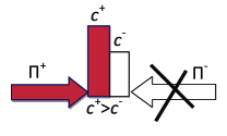
(a) $c>0$, the negative flux annihilates

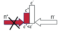
(b) $c<0$, the positive flux annihilates

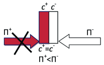
(c) $c=0$, the minimal flux annihilates

Figure 1: Annihilation of fluxes.

Proposition 1

$$\begin{split}\frac{{\mathrm{d}}}{{\mathrm{d}}t}\|G^{ij}(t)\|_{l_{1}}=&-\sum_{q,\ c^{+}_{q}>c^{-}_{q}}\Pi^{-}_{q}(t)-\sum_{q,\ c^{+}_{q}<c^{-}_{q}}\Pi^{+}_{q}(t)\\ &-\sum_{q,\ c^{+}_{q}=c^{-}_{q}}\min\{\Pi^{+}_{q}(t),\Pi^{-}_{q}(t)\}\ .\;\;\;\square\end{split}$$ (23)

Immediately from (23) we obtain the following integral formula

$$\begin{split}1-\|G^{ij}(t)\|_{l_{1}}=&\int_{t_{0}}^{t}\left(\sum_{q,\ c^{+}_{q}>c^{-}_{q}}\Pi^{-}_{q}(\tau)+\sum_{q,\ c^{+}_{q}<c^{-}_{q}}\Pi^{+}_{q}(\tau)\right.\\ &+\left.\sum_{q,\ c^{+}_{q}=c^{-}_{q}}\min\{\Pi^{+}_{q}(\tau),\Pi^{-}_{q}(\tau)\})\right)\ {\mathrm{d}}\tau\ .\end{split}$$ (24)

The annihilation formula gives us a better understanding of the nature of contraction but is not fully constructive because it uses fluxes from solutions to the initial kinetic equation (1).

4.2 Multi–Sheeted Extensions of Kinetic System

Let us introduce a multi–sheeted extension of a kinetic system.

Definition 2

The vertices of a multi–sheeted extension of the system (1) are $\mathcal{A}\times K$ where $K$ is a finite or countable set. An individual vertex is $(A_{i},l)$ ($l\in K$). The corresponding concentration is $c_{(i,l)}$. The reaction rate constant for $(A_{i},l)\to(A_{j},r)$ is $k_{(j,r)(i,l)}\geq 0$. This system is a multi–sheeted extension of the initial system if an identity holds:

$$\sum_{r}k_{(j,r)(i,l)}=k_{ji}\ \mbox{ for all }\ l\ .$$ (25)

This means that the flux from each vertex is distributed between sheets, but the sum through sheets is the same as for the initial system. We call the kinetic behavior of the sum $c_{i}=\sum_{l}c_{(i,l)}$ the base kinetics.

A simple proposition is important for further consideration.

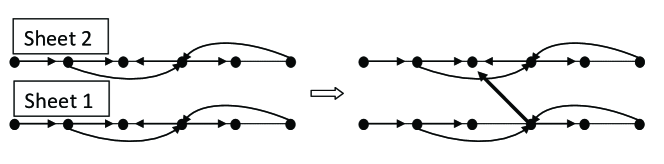
Figure 2: Redirection of a reaction from one sheet to another with preservation of the base kinetics. The redirected reaction is highlighted by bold.

Proposition 2

If $c_{(i,l)}(t)$ is a solution to the extended multi–sheeted system then

$$c_{i}(t)=\sum_{l}c_{(i,l)}(t)$$ (26)

is a solution to the initial system and

$$\sum_{il}|c_{(i,l)}(t)|\geq\sum_{i}|c_{i}(t)|\ .$$ (27)

(Here we do not assume positivity of all $c_{i}$).     $\square$

Formula (25) allows us to redirect reactions from one sheet to another (Fig. 2) without any change of the base kinetics. In the next section we show how to use this possibility for effective calculations.

Formula (26) means that kinetics of the extended system in projection on the initial space is the base kinetics: the components $(A_{i},l)$ are projected in $A_{i}$ the projected vector of concentrations is $c_{i}=\sum_{l}c_{(i,l)}$ and the projected kinetics is given by the initial Master equation with the projected coefficients $k_{ji}=\sum_{r}k_{(j,r)(i,l)}$. “Recharging” is any change of the non-negative extended coefficients $k_{(j,r)(i,l)}$ which does not change the projected coefficients.

The key role in the further estimates plays formula (27). We will apply this formula to the solutions with the zero sums of coordinates, they are differences between the normalized positive solutions.

4.3 Fluxes and Mixers

In this Subsection, we present the system of estimates for the contraction coefficient. The main idea is based on the following property which can be used as an alternative definition of weak ergodicity (Theorem 3): For each two vertices $A_{i},\>A_{j}\>(i\neq j)$ we can find a vertex $A_{q}$ that is reachable both from $A_{i}$ and from $A_{j}$. This means that the following structure exists:

$$A_{i}\to\ldots\to A_{q}\leftarrow\ldots\leftarrow A_{j}.$$

One of the paths can be degenerated: it may be $i=q$ or $j=q$. The positive flux from $A_{i}$ meets the negative flux from $A_{j}$ at point $A_{q}$ and one of them annihilates with the equal amount of the concentration of opposite sign.

Let us generalize this construction. Let us fix three different vertices: $A_{i}$ (the “positive source”), $A_{j}$ (the “negative source”) and $A_{q}$ (the “mixing point”). The degenerated case $q=i$ or $q=j$ we discuss separately. Let $S^{+}$ be such a system of vertices that $A_{i}\in S^{+}$, $A_{q}\notin S^{+}$ and there exists an oriented path in $S^{+}\cup\{A_{q}\}$ from $A_{i}$ to $A_{q}$. Analogously, let $S^{-}$ be such a system of vertices that $A_{j}\in S^{-}$, $A_{q}\notin S^{-}$ and there exists an oriented path in $S^{-}\cup\{A_{q}\}$ from $A_{j}$ to $A_{q}$. We assume that $S^{+}\cap S^{-}=\emptyset$.

With each subset of vertices $S$ we associate a kinetic system (subsystem): for $A_{r}\in S$

$$\dot{c}_{r}=\sum_{l,\ A_{l}\in S,\ r\neq l}k_{rl}c_{l}-\sum_{p=1}^{n}k_{pr}c_{r}\ .$$ (28)

In this subsystem, we retain all the outgoing reaction for $A_{r}\in S$ and delete the reactions which lead to vertices in $S$ from “abroad”.

The flux $\Pi_{S}^{+}$ from $S^{+}$ to $A_{q}$ is

$$\Pi_{S}^{+}=\sum_{r,\ A_{r}\in S^{+}}k_{qr}c_{r}(t)\ ,$$

where $c_{r}(t)$ is a component of the solution of (28) for $S=S^{+}$ with initial conditions $c_{r}(t_{0})=\delta_{ri}$. Analogously, we define the flux

$$\Pi_{S}^{-}=\sum_{r,\ A_{r}\in S^{-}}k_{qr}c_{r}(t)\ ,$$

where $c_{r}(t)$ is a component of the solution of (28) for $S=S^{-}$ with initial conditions $c_{r}(t_{0})=\delta_{rj}$. Decrease of the norm $\|G^{ij}(t)\|$ is estimated by the following theorem.

The system $S^{+},S^{-},A_{q}$ we call a mixer, that is a device for mixing. An elementary mixer consists of two kinetic paths $A_{i}\to\ldots\to A_{q}\leftarrow\ldots\leftarrow A_{j}$ (22) with the corespondent outgoing reactions:

$$\setcounter{MaxMatrixCols}{11}\begin{CD}A_{i_{1}}@>{k_{i_{2}i_{1}}}>{}>\ldots @>{k_{i_{r}i_{r-1}}}>{}>A_{i_{r}}@<{k_{i_{r}i_{r+1}}}<{}<\ldots @<{k_{i_{r+l-1}i_{r+l}}}<{}<A_{i_{r+l}}\\ @V{}V{\kappa_{i_{1}\overline{i_{2}}}}V@V{}V{\kappa_{i_{r}}}V@V{\kappa_{i_{r+l}{\overline{i_{r+l-1}}}}}V{}V\\ \end{CD}$$ (29)

where $i_{1}=i$, $i_{r}=q$, $i_{r+l}=j$.

The degenerated elementary mixer consists of one kinetic path:

$$\begin{CD}A_{i_{1}}@>{k_{i_{2}i_{1}}}>{}>A_{i_{2}}@>{k_{i_{3}i_{2}}}>{}>\ldots @>{k_{i_{r}i_{r-1}}}>{}>A_{i_{r}}\\ @V{}V{\kappa_{i_{1}\overline{i_{2}}}}V@V{}V{\kappa_{i_{2}\overline{i_{3}}}}V@V{}V{\kappa_{i_{r}}}V\\ \end{CD}$$ (30)

where $i_{1}=i$, $i_{r}=j$.

Theorem 4

$$\|G^{ij}(t)\|\leq 1-\int_{t_{0}}^{t}\min\{\Pi_{S}^{+},\Pi_{S}^{-}\}\ {\mathrm{d}}t\ .$$ (31)

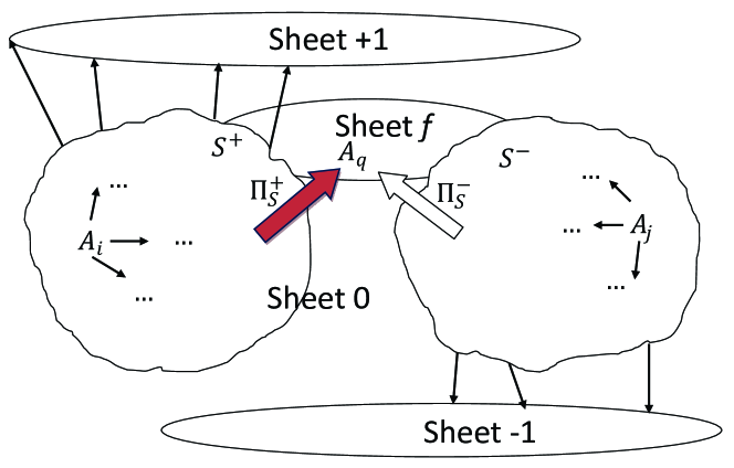
Figure 3: A mixer: two subsystems, $S^{+}$ (includes $A_{i}$) and $S^{-}$ (includes $A_{j}$). There may be outgoing reactions from $S^{\pm}$ but all incoming reactions to $S^{\pm}$ from outside are deleted. A mixing point $A_{q}$ and two fluxes, positive from $S^{+}$ (marked by dark color) and negative from $S^{-}$, meet at the mixing point.

Proof. To prove this theorem let us organize a 4–sheeted extension of the initial kinetic system as it is demonstrated in Fig. 3. Subsystems $S^{\pm}$ including the positive source (initial concentration $+1$) and the negative source (initial concentration $-1$) belong to level 0. Reactions from $S^{\pm}$ to $A_{q}$ are redirected to the sheet $f$, reactions from $S^{+}$ to other vertices, which do not belong to $S^{+}$, go to sheet $+1$, reactions from $S^{-}$ to other vertices, which do not belong to $S^{-}$, go to sheet $-1$. The incoming flux to the sheet $f$ is $\Pi_{S}^{+}-\Pi_{S}^{-}$.

Let us introduce the following notations:

$$C_{S}^{+}=\sum_{A_{p}\in S^{+}}c_{(p,0)}+\sum_{q=1}^{n}c_{(q,1)}\ ;$$

$$C_{S}^{-}=-\sum_{A_{p}\in S^{-}}c_{(p,0)}-\sum_{q=1}^{n}c_{(q,-1)}\ ;$$

$$C_{f}=\sum_{r=1}^{n}|c_{(r,f)}|\ .$$

We consider solution to the kinetic equations for the multi–sheeted system with initial conditions: $c_{(i,0)}(t_{0})=1$, $c_{(j,0)}(t_{0})=-1$ and all other concentrations are equal to zero at time $t_{0}$. In this case, some of the signs of concentrations are known for $t\geq t_{0}$ due to the organization of the redirection of reactions (Fig. 3):

$$\begin{split}&c_{(p,0)}\geq 0\ \ \mbox{for}\ \ A_{p}\in S^{+}\ ,\ \ c_{(p,0)}\leq 0\ \ \mbox{for}\ \ A_{p}\in S^{-}\ ,\\ &c_{(p,0)}=0\ \ \mbox{for}\ \ A_{p}\notin S^{+}\cup S^{-}\ ,\\ &c_{(q,1)}\geq 0,\ \ c_{(q,-1)}\leq 0\ .\end{split}$$ (32)

Let us use (8) for $S^{+}$ with the sheet $+1$ and for $S^{-}$ with the sheet $-1$. We get immediately

$$\frac{{\mathrm{d}}C_{S}^{+}}{{\mathrm{d}}t}=\Pi_{S}^{+}\ ,\ \ \frac{{\mathrm{d}}C_{S}^{-}}{{\mathrm{d}}t}=\Pi_{S}^{-}$$ (33)

Analogously, we can use (9) for the sheet $f$ and get

$$\frac{{\mathrm{d}}C_{f}}{{\mathrm{d}}t}\leq|\Pi_{S}^{+}-\Pi_{S}^{-}|\ .$$ (34)

For the norm of the base vector of concentration $c$ the inequality holds (Proposition 2):

$$\|c\|\leq C^{+}_{S}+C^{-}_{S}+C_{f}\ .$$

Finally, we combine this inequality with (33), (34) and get

$$\|c(t)\|\leq 2-2\int_{t_{0}}^{t}\min\{\Pi_{S}^{+}(\tau),\Pi_{S}^{-}(\tau)\}\ {\mathrm{d}}\tau\ \ \ \ \square$$

For the degenerate case the path from $A_{i}$ goes directly to $A_{j}$ (or inverse). let us assume that there is a subsystem $S^{+}$, $A_{i}\in S^{+}$, the mixing point $A_{q}$ coincides with $A_{j}$ and the flux $\Pi^{+}_{S}$ is

$$\Pi_{S}^{+}=\sum_{r,\ A_{r}\in S^{+}}k_{jr}c_{r}(t)\ ,$$

where $c_{r}(t)$ is a component of the solution of (28) for $S=S^{+}$ with initial conditions $c_{r}(t_{0})=\delta_{ri}$.

Theorem 5

$$\|G^{ij}(t)\|\leq 1-\int_{t_{0}}^{\min\{t,t_{1}\}}{\Pi_{S}^{+}(\tau)}\ {\mathrm{d}}\tau,$$ (35)

where $\kappa_{j}=\sum_{p}k_{pj}$ and $t_{1}$ is a solution to equation

$$\int_{t_{0}}^{t}{\Pi_{S}^{+}}(\tau)\exp(-\kappa_{j}(t-\tau))\ {\mathrm{d}}\tau=\exp(-\kappa_{j}t)\ .$$ (36)

Proof. This theorem is also proved by the construction of the appropriate multi–sheeted extension of the kinetic system. For the degenerated case we need only two additional sheets: subsystem $S^{+}$ including the positive source $A_{i}$ (initial concentration $+1$) and the negative source $A_{j}$ (initial concentration $-1$) belong to level 0. Reactions from $S^{+}$ to other vertices, which do not coincide with $A_{j}$, go to sheet $+1$, reactions from $A_{j}$ to other vertices go to sheet $-1$. The concentration of $A_{(j,0)}$ is

$$c_{(j,0)}(t)=\int_{t_{0}}^{t}{\Pi_{S}^{+}}(\tau)\exp(-\kappa_{j}(t-\tau))\ {\mathrm{d}}\tau-\exp(-\kappa_{j}t)\ .$$

Let us introduce the following notation:

$$C_{S}^{+}=\sum_{A_{p}\in S^{+}}c_{(p,0)}+\sum_{q=1}^{n}c_{(q,1)}\ ;$$

$$C^{-}=-c_{(j,0)}-\sum_{q=1}^{n}c_{(q,-1)}\ .$$

For $t\leq t_{1}$ concentrations $c_{(j,0)}(t)$ and all $c_{(q,-1)}$ are negative, hence

$$\frac{{\mathrm{d}}C_{S}^{+}}{{\mathrm{d}}t}=\frac{{\mathrm{d}}C^{-}}{{\mathrm{d}}t}=-\Pi_{S}^{+}(t)$$ (37)

and for the norm of the correspondent solution for the base system we get the inequality

$$\|c(t)\|\leq 2-2\int_{t_{0}}^{\min\{t,t_{1}\}}{\Pi_{S}^{+}(\tau)}\ {\mathrm{d}}\tau\ \ \ \ \ \square$$ (38)

The kinetic path summation formula gives us a family of estimates of $\Pi_{S}^{\pm}$ from below. For each pair $i,j$ we can find the best of available estimates of $\|G^{ij}(t)\|$ (the smallest one for various choices of $A_{q}$ and subsets $S^{\pm}$) and then among all pairs of $i,j$ we should choose the “most pessimistic” evaluation of $\|G^{ij}(t)\|$ (the biggest one). It will give the evaluation of the contraction coefficient from above.

5 Simple example: Irreversible Cycle

Let us demonstrate all results for a simple kinetic system, a simple irreversible cycle:

$$A_{1}\xrightarrow{k_{1}}A_{2}\xrightarrow{k_{2}}\ldots\xrightarrow{k_{n-1}}A_{n}\xrightarrow{k_{n}}A_{1}$$ (39)

All $k_{i}>0$ and are constant in time. For enumeration of $A_{i}$ we use the standard cyclic order (mod$n$): $A_{n+j}\equiv A_{j}$.

The kinetic equations for this system are: $\dot{c}=Kc$ or

$$\frac{{\mathrm{d}}}{{\mathrm{d}}t}\left[\begin{array}[]{l}c_{1}\\ c_{2}\\ \vdots\\ c_{n}\end{array}\right]=\left[\begin{array}[]{llll}-k_{1}&0&\ldots&k_{n}\\ k_{1}&-k_{2}&\ldots&0\\ \vdots&\vdots&\vdots&\vdots\\ 0&0&0&-k_{n}\end{array}\right]\,\left[\begin{array}[]{l}c_{1}\\ c_{2}\\ \vdots\\ c_{n}\end{array}\right]$$ (40)

The characteristic equation for this system is

$$\prod_{i=1}^{n}(k_{i}+\lambda)=\prod_{i=1}^{n}k_{i}\,.$$

One eigenvalue for matrix $K$ is, obviously, $\lambda=0$, the correspondent left eigenvector is the linear conservation law $l_{1}=(1,1,\ldots,1)$. The right eigenvector for this $\lambda$ is the steady state $r_{1}=\frac{1}{\sum_{i}\frac{1}{k_{i}}}(\frac{1}{k_{1}},\frac{1}{k_{2}},\ldots,\frac{1}{k_{n}})^{\rm T}$ (normalized for $l_{1}r_{1}=1$). Other $n-1$ roots of the characteristic equations have strictly negative real parts, $Re\lambda_{i}<0$ ($i>1$) and, in general, cannot be found explicitly. For a given eigenvalue $\lambda$, the eigenvectors have a simple structure:

$$l_{{\lambda}\,i+1}=l_{{\lambda}\,i}\frac{\lambda+k_{i}}{k_{i}}\,\;\;r_{{\lambda}\,i}=\frac{\psi_{{\lambda}\,i}}{k_{i}}\,,\,\,\psi_{{\lambda}\,i-1}=\psi_{{\lambda}\,i}\frac{\lambda+k_{i}}{k_{i}}\,.$$ (41)

With the normalization condition: for eigenvalues $\lambda$, $\lambda^{\prime}$: $l_{\lambda}r_{\lambda^{\prime}}=\delta_{\lambda\lambda^{\prime}}$, that is 1 for $\lambda=\lambda^{\prime}$ and 0 for $\lambda\neq\lambda^{\prime}$.

Two limit cases allow explicit analysis of eigenvalues and eigenvectors of $K$:

1. Systems with limiting steps: one constant is much smaller than others, let it be $k_{n}$, $k_{n}\ll k_{i}$, ($i=1,\ldots,n-1$);

2. Fully symmetric systems, $k_{1}=k_{2}=\ldots=k_{n}$.

For systems with limiting steps ($k_{n}\ll k_{i}$, ($i=1,\ldots,n-1$)) the eigenvalues are close to $-k_{1},\ldots,-k_{n-1}$ and the relaxation is limited by the second constant, the next to the minimal one (detailed analysis is provided in [11, 12]).

For a symmetric system ($k_{1}=k_{2}=\ldots=k_{n}=k$), the eigenvalues are: $\lambda_{q}=k\exp\left(\frac{2\pi iq}{n}\right)-1$ for $q=1,\ldots,n$. There are $n$ distinct eigenvalues, one of them, $\lambda_{n}=0$, the other have negative real part: $Re\lambda_{q}=k\left[\cos\left(\frac{2\pi iq}{n}\right)-1\right]$. Let us further take $k=1$ for this system (include $k$ into dimensionless time). For the left and right eigenvectors (41) we have two waves moving in opposite directions, $l_{q\,j+1}=l_{qj}\exp\left(\frac{2\pi iq}{n}\right)$, $r_{q\,j-1}=r_{q\,j}\exp\left(\frac{2\pi iq}{n}\right)$. We can take with respect to the normalization condition, $l_{q}r_{p}=\delta_{qp}$:

$$\begin{split}&l_{q}=\left(1,\exp\left(\frac{2\pi iq}{n}\right),\exp\left(2\frac{2\pi iq}{n}\right),\ldots,\exp\left((n-1)\frac{2\pi iq}{n}\right)\right)\,,\\ &r_{q}=\frac{1}{n}\left(1,\exp\left(-\frac{2\pi iq}{n}\right),\exp\left(-2\frac{2\pi iq}{n}\right),\ldots,\exp\left(-(n-1)\frac{2\pi iq}{n}\right)\right)^{\rm T}\,.\end{split}$$ (42)

For constant coefficients, the operator of shift in time from $t_{0}$ to $t_{1}$ depends only on $t=t_{1}-t_{0}$: $U(t_{1},t_{0})=U(t)=\exp Kt$. We can use (42) and write

$$\begin{split}&U(t)=\sum_{q=1}^{n}\exp(\lambda_{q}t)|r_{q}\rangle\langle l_{q}|\,,\\ &(U(t))_{js}=\sum_{q=1}^{n}\exp(\lambda_{q}t)r_{qj}l_{qs}\\ &\qquad\quad=\frac{1}{n}\sum_{q=1}^{n}\exp\left[t\left(\cos\frac{2\pi q}{n}-1\right)\right]\cos\left((s-j)\frac{2\pi q}{n}+t\sin\frac{2\pi q}{n}\right)\,.\end{split}$$ (43)

This explicit formula allows us to compute all the necessary quantities including the contraction coefficient $\delta_{U(t)}$ (4).

Now, let us produce the approximate formula for the same symmetric system by mixers. First of all, let us represent the solution for the cycle by the path summation formula. With the convention of cyclic enumeration, the set of paths $\mathcal{I}_{i}$ started at $A_{i}$ is the sequence

$$\mathcal{I}_{i}=\left\{\begin{array}[]{l}A_{i}\xrightarrow{k_{i}}\,,\\ A_{i}\xrightarrow{k_{i}}A_{i+1}\xrightarrow{k_{i+1}}\,,\\ \cdots\cdots\cdots\cdots\cdots\cdots\cdots\cdots\\ A_{i}\xrightarrow{k_{i}}A_{i+1}\xrightarrow{k_{i+1}}A_{i+2}\xrightarrow{k_{i+2}}\ldots\xrightarrow{k_{i+j-1}}A_{i+j+1}\xrightarrow{k_{i+j}}\,,\\ \cdots\cdots\cdots\cdots\cdots\cdots\cdots\cdots\end{array}\right\}\,.$$ (44)

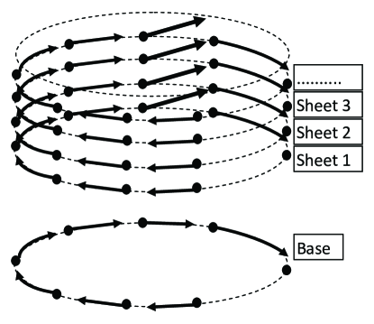
Figure 4: Multi–sheeted representation of the path summation formula for a cycle (46): a cycle (the base) is represented by an semi-infinite helix produced by redirecting of reactions between sheets.

This sequence of paths corresponds to the multi–sheeted representation presented in Fig. 4. First, we consider a infinite series of the copies of the cycle. Each vertex of the extended system is numerated by two indexes: $(A_{i},l)$, $i=1,2,\ldots,n$ (mod$n$), $l=1,2,3,\ldots$ is a natural number. The reaction rate constants for copies are the same as for the initial systems: $k_{(j,r)(i,l)}=k_{ji}\delta_{rl}$. This extended system obviously satisfies the definition of the multi–sheeted extension of the cycle and in its projection on the base we always have the kinetics of the cycle.

Let us select one number $i\in\{1,\ldots,n\}$ and recharge the reactions: we annulate the “horizontal” reaction rate constant for $(A_{i},l)\to(A_{i+1},l)$, $k_{(i+1,l)(i,l)}=0$, and instead of this reaction take the reaction between levels, $(A_{i},l)\to(A_{i+1},l+1)$: $k_{(i+1,l+1)(i,l)}=k_{i+1\,i}$ (see Fig. 4). This is also a multi–sheeted extension of the cycle. Formula (26) for this multi–sheeted system allows us to use integration of the infinite acyclic system (represented by the spiral in Fig. 4)) instead of integration of the finite cyclic base system.

Now, let us put all $k_{i}=1$. For systems with constant coefficients we use initial time moment $t_{0}=0$. For the set of paths $\mathcal{I}_{i}$ started at $A_{i}$ the solution to the chain (11) with the initial conditions $\varsigma_{i}(t_{0})=1$ and $\varsigma_{I}=0$ for $|I|>1$ is

$$\varsigma_{I}(t)=\frac{t^{|I|-1}}{(|I|-1)!}e^{-t}\ .$$ (45)

Obviously, $\sum_{I\in\mathcal{I}_{i}}\varsigma_{I}=1$. For concentration of $A_{q}$, formula (17) gives

$$u_{ji}(t)=e^{-t}\sum_{q=0}^{\infty}\frac{t^{qn+d_{ij}}}{(qn+d_{ij})!}\ ,$$ (46)

where $d_{ij}$ is the length of the shortest oriented path from $A_{i}$ to $A_{j}$ (here the length is the number of reactions and the trivial path from $A_{i}$ to $A_{i}$ has the length zero).

For every two vertices $A_{i}$, $A_{j}$ we have only two mixers and both are degenerated: $A_{i}\xrightarrow{k}A_{i+1}\xrightarrow{k}\ldots\xrightarrow{k}A_{j}\xrightarrow{k}$, length $j-i\mod n$ and $A_{j}\xrightarrow{k}A_{j+1}\xrightarrow{k}\ldots\xrightarrow{k}A_{i}\xrightarrow{k}$, length $i-j\mod n$.

Let us select one mixer $A_{1}\xrightarrow{k}A_{2}\ldots\xrightarrow{k}A_{j}\xrightarrow{k}$ for analysis. Initial conditions are: $c_{1}=1$, $c_{j}=-1$ and other concentrations are equal to zero.

For this auxiliary chain with given initial conditions

$$\begin{split}&c_{p}=\frac{t^{p-1}}{(p-1)!}e^{-t}\ \ (p=1,\ldots,j-1),\\ &c_{j}=-e^{-t}\left(1-\frac{t^{j-1}}{(j-1)!}\right)\ .\end{split}$$ (47)

The estimate (35) $\|G^{ij}(t)\|\leq 1-\int_{0}^{t}{\Pi_{S}^{+}(\tau)}\ {\mathrm{d}}\tau$ is valid until $c_{j}$ changes its sign. Hence, for $t$ we have a boundary $t^{j-1}\leq(j-1)!$. The Stirling formula gives a convenient estimate:

$$\begin{split}&t^{j-1}\leq\sqrt{2\pi(j-1)}\left(\frac{j-1}{e}\right)^{j-1}\lesssim(j-1)!\\ &t\leq t_{1}=\frac{j-1}{e}(2\pi(j-1))^{\frac{1}{2(j-1)}}\ .\end{split}$$ (48)

Even a simpler estimate is $t<(j-1)/e$. If $t$ satisfies one of these inequalities then concentration $c_{j}$ is negative and we can use the estimate (35).

For this example,

$$\begin{split}&\Pi_{S}^{+}(t)=c_{j-1}(t)=\frac{t^{j-2}}{(j-2)!}e^{-t}\ ,\;\int_{0}^{t}{\Pi_{S}^{+}(\tau)}\ {\mathrm{d}}\tau=1-e^{-t}\sum_{p=0}^{j-2}\frac{t^{p}}{p!}\ ,\\ &\|G^{ij}(t)\|\leq e^{-t}\sum_{p=0}^{\min\{d_{ji},d_{ij}\}-1}\frac{t^{p}}{p!}\,,\;\delta_{U(t)}\leq e^{-t}\sum_{p=0}^{\left[\frac{n}{2}\right]}\frac{t^{p}}{p!}\,,\end{split}$$ (49)

where $\left[\frac{n}{2}\right]$ is the integer part of $n/2$. For $t>0$ this estimate gives $\|G^{ij}(t)\|<1$ and $\delta_{U(t)}<1$ because $\sum_{p=0}^{j-2}\frac{t^{p}}{p!}<e^{t}$. We can use the estimate (LABEL:cycleestimeG) on an interval $[0,t_{1}]$, for example, on $[0,\frac{j-1}{e}]$. Intersection of these intervals for all $i,j,i\neq j$ is $[0,\frac{1}{e}]$ ($j\geq 2$). On this interval, the estimate (LABEL:cycleestimeG) is valid for all $i,j$. For extension of such an estimate for $t>\frac{1}{e}$ the submultiplicative property (5) can be used.

6 Ergodicity Boundary and Limitation of Ergodicity

In this Section we consider a reaction kinetic system (1) with constant coefficients $k_{ji}>0$ for $(i,j)\in\mathcal{E}$.

Let us sort the values of kinetic parameters in decreasing order: $k_{(1)}>k_{(2)}>\ldots>k_{(n)}$. The number in parenthesis is the number of value in this order. Each of the constants $k_{(q)}$ is a reaction rate constant $k_{ij}$ for some $i,j$ (and may be for several of them if values of these constants coincide). Let us also suppose that the network is weakly ergodic. We say that $k_{(r)},\,1\leq r\leq n$ is the ergodicity boundary [18] if the network of reactions with parameters $k_{1},k_{2},\ldots,k_{r}$ is weakly ergodic, but the network with parameters $k_{1},k_{2},\ldots,k_{r-1}$ is not. In other words, when eliminating reactions in decreasing order of their characteristic times, starting with the slowest one, the ergodicity boundary is the constant of the first reaction whose elimination breaks the ergodicity of the reaction digraph.

Let $\mathcal{M}_{ij}$ ($i\neq j$) be a set of elementary mixers (29), (30) between given $A_{i}$, $A_{j}$. For each $M\in\mathcal{M}_{ij}$ we can find a cutting reaction rate constant, ${\rm cut}_{M}$:

$$\begin{split}{\rm cut}_{M}=\min\{k_{i_{2}i_{1}},\ldots,k_{i_{r}i_{r-1}},k_{i_{r}i_{r+1}},\ldots,k_{i_{r+l-1}i_{r+l}}\}\ \ \mbox{for (\ref{ElementaryMixer})}\ ;\\ {\rm cut}_{M}=\min\{k_{i_{2}i_{1}},\ldots,k_{i_{r}i_{r-1}}\}\ \ \mbox{for (\ref{ElementaryMixerDegen})}\ .\end{split}$$ (50)

Let us eliminate reactions in increasing orders of their constants (i.e. in decreasing order of their characteristic times), starting with the smallest one. To cut all elementary mixers between $A_{i},A_{j}$ ($i\neq j$), it is necessary and sufficient to eliminate all $k_{pq}\leq{\rm cut}_{M}$ for all $M\in\mathcal{M}_{ij}$. Therefore, for every pair $A_{i},A_{j}$ ($i\neq j$) we can also introduce a cutting constant:

$${\rm cut}_{ij}=\max_{M\in\mathcal{M}_{ij}}{\rm cut}_{M}\ .$$

To destroy the weak ergodicity of the network $\mathcal{N}$ we have to cut al least one pair $A_{i},A_{j}$ ($i\neq j$). The result can be formulates as the following theorem.

Theorem 6

Theorem 6 The ergodicity boundary of a network $\mathcal{N}$ is the following constant:

$${\rm cut}_{\mathcal{N}}=\min_{i\neq j}{\rm cut}_{ij}\ .\ \ \ \ \ \ \ \square$$

This boundary is a minimum (in pairs $A_{i},A_{j}$) of maxima (in mixers $M\in\mathcal{M}_{ij}$) of minima (in constants).

Kinetic equations for elementary mixers (29), (30) allow explicit analytic solutions. Nevertheless, explicit estimates in terms of cutting constants can be also useful.

Let for an elementary mixer $M$ (29) $\kappa_{M}$ be the maximal sum of constants of outgoing reactions:

$$\kappa_{M}=\max\{\kappa_{i_{p}}\ |\ p=i_{1},i_{2},\ldots,i_{r+l}\},\ \ \kappa_{s}=\sum_{p,\ p\neq s}k_{ps}\ ,$$

or for a degenerated elementary mixer $M$ (30)

$$\kappa_{M}=\max\{\kappa_{i_{p}}\ |\ p=i_{1},i_{2},\ldots,i_{r}\}\ .$$

Let us substitute all the constant for horizontal arrows in the elementary mixer $M$ (29), (30) by $k={\rm cut}_{M}$, and all the constants for vertical arrows ($i\neq i_{r}$) by $\kappa-k$, where $\kappa=\kappa_{M}$. This change decreases the fluxes $\Pi^{\pm}$.

To find the estimate we have to solve the kinetic equation for a simple uniform kinetic path:

$$\setcounter{MaxMatrixCols}{11}\begin{CD}A_{1}@>{k}>{}>A_{2}@>{k}>{}>\ldots @>{k}>{}>A_{s}@>{k}>{}>\\ @V{}V{\kappa-k}V@V{}V{\kappa-k}V@V{}V{\kappa-k}V\\ \end{CD}$$ (51)

Similar to the simple cycle (47), we find

$$c_{p}=\frac{(kt)^{p-1}}{(p-1)!}\exp(-\kappa t)\ \ (p=1,\ldots,s)\ ,$$ (52)

the only difference is in exponents.

For the elementary mixers (29), (30) this formula gives

$$\Pi^{+}(t)\geq k\frac{(kt)^{r-2}}{(r-2)!}\exp(-\kappa t)\ ,\ \ \Pi^{-}(t)\geq k\frac{(kt)^{l-1}}{(l-1)!}\exp(-\kappa t)\$$

and the estimates from Theorems 4,5 (31), (35) become simple analytical expressions after substitution of $\Pi^{\pm}$ by their estimates from below.

Let us find an universal estimate from below for $t_{1}$. It is

$$\vartheta=\frac{1}{k+\kappa}\ .$$

Indeed, in the degenerated elementary mixer (30) on the way from $A_{i}$ to $A_{j}$ there exists at least one reaction with reaction rate constant $k$: $A_{r}\to\ldots$. The integral flux through this reaction during the time interval $[0,t]$ is

$$\int_{0}^{t}kc_{r}(\tau)\ {\mathrm{d}}\tau\geq\int_{0}^{t}\Pi^{+}(\tau)\ {\mathrm{d}}\tau\ .$$

The last inequality holds because all the flux in the mixer should go through the reaction $A_{r}\to\ldots$ before it enters the last vertex. On the other hand, $\int_{0}^{t}kc_{r}(\tau)\ {\mathrm{d}}\tau\leq\int_{0}^{t}k\exp(-k\tau)\ {\mathrm{d}}\tau$ (the last integral corresponds to the case when all the concentration is collected at the initial moment at $A_{r}$ and goes only through the reaction $A_{r}\to\ldots$). Therefore,

$$\int_{0}^{t}\Pi^{+}(\tau)\ {\mathrm{d}}\tau\leq 1-\exp(-k\tau)\ .$$

From the condition (36) we find the estimate for $t_{1}$ from below: $t_{1}\geq\tau_{1}$, where $\tau_{1}$ is solution to

$$1-\exp(-k\tau)=\exp(-\kappa\tau)\ .$$

We use convexity of exponential functions and substitute them in this equation by linear approximation at point $\tau=0$: $\exp(-x)>1-x$ ($x>0$); this gives us the estimate of $\tau_{1}$ from below: $\tau_{1}<\vartheta=\frac{1}{k+\kappa}$.

For $t\in[0,\vartheta]$, $kt<1$ and

$$1=\frac{(kt)^{0}}{0!}>\frac{(kt)^{1}}{1!}>\ldots>\frac{(kt)^{r}}{r!}>\ldots\ .$$

For each mixer $M$ we introduce the length of mixer $d_{M}=\max\{r-2,l-1\}$ for (29) and $d_{M}=r-2$ for (30). In these notations, each mixer $M\in\mathcal{M}_{ij}$ gives the estimate: for $t\in[0,\vartheta_{M}]$

$$\|G^{ij}(t)\|\leq 1-\int_{0}^{t}{\rm cut}_{M}\frac{({\rm cut}_{M}\tau)^{d_{M}}}{(d_{M})!}\exp(-\kappa_{M}\tau)\ {\mathrm{d}}\tau\ ,$$ (53)

where

$$\vartheta_{M}=\frac{1}{{\rm cut}_{M}+\kappa_{M}}\ .$$

For each pair $i,j$ ($i\neq j$) we can select the “critical” elementary mixer $M\in\mathcal{M}_{ij}$ with ${\rm cut}_{M}={\rm cut}_{ij}$ and put $d_{ij}=d_{M}$, $\kappa_{ij}=\kappa_{M}$. If there are several critical elementary mixers then we select one with minimal $d_{M}$, if there are several such a mixers with minimal $d_{M}$ then we select one with minimal $\kappa_{M}$. In this notation we have

$$\|G^{ij}(t)\|\leq 1-\int_{0}^{t}{\rm cut}_{ij}\frac{({\rm cut}_{ij}\tau)^{d_{ij}}}{(d_{ij})!}\exp(-\kappa_{ij}\tau)\ {\mathrm{d}}\tau\$$ (54)

for $t\in[0,\vartheta_{ij}]$, where

$$\vartheta_{ij}=\frac{1}{{\rm cut}_{ij}+\kappa_{ij}}\ .$$

Finally, for the whole network $\mathcal{N}$

$${\rm cut}_{\mathcal{N}}=\min_{i,j,i\neq j}\{{\rm cut}_{ij}\},\ d_{\mathcal{N}}=\max_{i,j,i\neq j}\{d_{ij}\},\ \kappa_{\mathcal{N}}=\max_{i,j,i\neq j}\{\kappa_{ij}\},\ \vartheta_{\mathcal{N}}=\frac{1}{{\rm cut}_{\mathcal{N}}+\kappa_{\mathcal{N}}}$$

and for the contraction coefficient $\delta(t)$ (21) we obtain the estimate

$$\begin{split}\delta(t)\leq&1-\int_{0}^{t}{\rm cut}_{\mathcal{N}}\frac{({\rm cut}_{\mathcal{N}}\tau)^{d_{\mathcal{N}}}}{(d_{\mathcal{N}})!}\exp(-\kappa_{\mathcal{N}}\tau)\ {\mathrm{d}}\tau\\ &=1-\left(\frac{{\rm cut}_{\mathcal{N}}}{\kappa_{\mathcal{N}}}\right)^{d_{\mathcal{N}}+1}\left[1-\sum_{p=0}^{d_{\mathcal{N}}}\frac{(\kappa_{\mathcal{N}}t)^{p}}{p!}\exp(-\kappa_{\mathcal{N}}t)\right]\end{split}$$ (55)

for $t\in[0,\vartheta_{\mathcal{N}}]$. For $t$ outside this interval, the submultiplicative property (5) should be used.

7 Discussion

The kinetic path summation formula together with the multi–sheeted extension of kinetics provide us with a factory of estimates. It is difficult to find, who invented this approach.

The analysis of kinetic paths with selection of the most important (dominant) paths allowed us to extract dominant systems from kinetic equations [11, 12]. A robust procedure for simplification of biochemical networks was created [19]. This approach was developed into unified framework for hybrid simplifications of Markov models of multiscale stochastic gene networks dynamics [20]. Dominant subsystems were analyzed for dynamical models of microRNA action on the protein translation process [21].

The multi–sheeted extension of kinetics provides us with a simple and useful technique for estimation of relaxation processes in Master equation. This method introduces an internal “microstructure” in the first order kinetic systems. The kinetic path summation formula is a particular case of the formula (26) (Proposition 2).

Indeed, let us construct the following multi–sheeted extension of the Master equation. The set of components is $\mathcal{A}\times\mathcal{K}$, where $\mathcal{K}=\{0\}\cup\mathcal{K}_{1}$ and $\mathcal{K}_{1}$ is the set of all kinetic paths $I$ with lengths $|I|>1$ (non-degenerated paths). The connections between sheets (redirected reactions) are:

$$A_{i_{I^{-}},I^{-}}\xrightarrow{k_{I}}A_{i_{I},I}\ \ \mbox{instead of}\ \ A_{i_{I^{-}},I^{-}}\xrightarrow{k_{I}}A_{i_{I},I^{-}}\ .$$

According to this rule, the reaction that continues the path $I^{-}$ to the path $I$ is redirected and goes from the sheet $I^{-}$ to the sheet $I$. For a degenerated $I^{-}$, we take $A_{i_{I^{-}},I^{-}}=A_{i_{I^{-}},0}$, this means that all paths start on the zero sheet, and all reactions from this sheet lead to other sheets: $A_{i}\to A_{j}$ transforms into $A_{i,0}\to A_{j,\{i,j\}}$, where $\{i,j\}$ is a path of the length 2. Formula (26) for this multi–sheeted structure coincide with the kinetic path summation formula (17) (Theorem 2) for initial conditions $c_{i,0}=1$ and other $c_{(j,I)}=0$.

This multi–sheeted extension may be considered as a generalization of the Bethe lattices introduced by H. Bethe in 1935 [22]. For example, if in the initial graph of reactions each vertex has the same number of outgoing edges then the constructed multi–sheeted extension can be considered as a bundle of the Bethe lattices, each of them starts from one point of the zeroth sheet. For each starting point, $A_{(i,0)}$ the corresponding Bethe lattice represents the “Green function” $u_{ji}(t,t_{0})$ for given $i$ and for all possible $j$.

We produced the kinetic path summation formula for time–dependent kinetic equations and applied this formula for evaluation of the ergodicity coefficient. The evaluation of the contraction coefficient in the $l_{1}$ norm is the main tool for studying of the relaxation in time–dependent Markov processes since the seminal works of R. Dobrushin [15].

Another important context of this study is the analysis of the eigenvalues of the stochastic matrices [23, 24] and, especially the analysis of these eigenvalues for matrices with specified graph [25, 26]. In chemical kinetics, evaluation of the eigenvalues through kinetic constants was given in series of work by V.Cheresiz and G. Yablonskii [27, 28].

Various estimates of eigenvalues of $K$ could be produced from the estimates of contraction (31), (35). The simplest one follows from (55):

$$Re(\lambda)\leq\frac{\ln(\delta(\vartheta))}{\vartheta}<0\ .$$ (56)

Several problems should be resolved to make the use of the path summation formula more effective. Perhaps, the most important of them was mentioned in the comment [29]). The amount of the kinetic path needed for accurate estimate of the solution grows quickly in time for a sufficiently complex system. Hence, we need either special tricks for the analysis of path sampling or special asymptotic formulas for long paths instead of exact solutions.

Another possible approach to this problem is in the use of more complex exactly solvable systems instead of paths. The set of reactions is solvable, if there exists a linear transformation of coordinates $c\mapsto a$ such that kinetic equations in new coordinates for all values of reaction constants have the triangle form:

$$\frac{{\mathrm{d}}a_{i}}{{\mathrm{d}}t}=f_{i}(a_{1},a_{2},...\,a_{i}).$$ (57)

The algorithm for the analysis of reaction network solvability was developed in [5] (see also [11]). The simplest examples of solvable networks give acyclic graphs (reaction trees) and pairs of mutually inverse reactions. It may be possible to decompose the complex system of transitions into a sequence of solvable systems.

References

- [1] S.R. Meyn, Control Techniques for Complex Networks, Cambridge University Press, Cambridge, 2007.
- [2] S.R. Meyn, R.L. Tweedie, Markov Chains and Stochastic Stability, 2nd Edition, Cambridge University Press, Cambridge, 2009.
- [3] N.G. Van Kampen, Stochastic processes in physics and chemistry, North–Holland, Amsterdam 1981.
- [4] J.C. Kuo, J. Wei, A lumping analysis in monomolecular reaction systems. Analysis of the approximately lumpable system. Ind. Eng. Chem. Fundam. 8 (1969) 124–133.
- [5] A.N. Gorban, V.I. Bykov, G.S. Yablonskii, Essays on chemical relaxation, Novosibirsk: Nauka, 1986.
- [6] S.X. Sun, Path Summation Formulation of the Master Equation, Phys. Rev. Lett. 96 (2006), 210602.
- [7] B. Harland, S.X. Sun, Path ensembles and path sampling in nonequilibrium stochastic systems, J. Chem. Phys. 127 (2007), 104103.
- [8] D.T. Gillespie, Exact Stochastic Simulation of Coupled Chemical Reactions, J. Phys. Chem. 81 (25) (1977), 2340–2361.
- [9] O. Flomenbom, J. Klafter, Closed-Form Solutions for Continuous Time Random Walks on Finite Chains, Phys. Rev. Lett. 95 (2005), 098105.
- [10] O. Flomenbom, R.J. Silbey, Path-probability density functions for semi-Markovian random walks, Phys. Rev E 76 (2007), 041101.
- [11] A.N. Gorban, O. Radulescu, Dynamic and static limitation in reaction networks, revisited, Advances in Chemical Engineering 34 (2008), 103–173. E-print: arXiv:physics/0703278 [physics.chem-ph]
- [12] A.N. Gorban, O. Radulescu, A.Y. Zinovyev, Asymptotology of chemical reaction networks, Chemical Engineering Science 65 (2010), 2310–2324. E-print: arXiv:0903.5072 [physics.chem-ph]
- [13] G.S. Yablonskii, V. I. Bykov, A.N. Gorban, V.I. Elokhin, Kinetic models of catalytic reactions (Series Comprehensive Chemical Kinetics, Vol. 32), Elsevier, Amsterdam, 1991.
- [14] O.N. Temkin, A.V. Zeigarnik, D.G. Bonchev, Chemical Reaction Networks: A Graph-Theoretical Approach, CRC Press, Boca Raton, FL, 1996.
- [15] R.L. Dobrushin, Central limit theorem for non-stationary Markov chains I, II, Theor. Prob. Appl. 1 (1956), 163–80, 329–383.
- [16] E. Seneta, Nonnegative Matrices and Markov Chains, Springer, New York, 1981.
- [17] P. Van Mieghem, Performance Analysis of Communications Networks and Systems, Cambridge University Press, Cambridge, 2006.
- [18] A.N. Gorban, O. Radulescu, Dynamical robustness of biological networks with hierarchical distribution of time scales, IET Syst. Biol., 1 (2007), 238–246. E-print: arXiv:q-bio/0701020 [q-bio.MN].
- [19] O. Radulescu, A.N. Gorban, A. Zinovyev, A. Lilienbaum, A. Robust simplifications of multiscale biochemical networks, BMC Systems Biology 2 (1) (2008), 86. http://www.biomedcentral.com/1752-0509/2/86
- [20] A. Crudu, A. Debussche and O. Radulescu, Hybrid stochastic simplifications for multiscale gene networks, BMC Systems Biology, 3 (2009), 89. http://www.biomedcentral.com/1752-0509/3/89/
- [21] A. Zinovyev, N. Morozova, N. Nonne, E. Barillot, A. Harel-Bellan, A.N. Gorban, Dynamical modeling of microRNA action on the protein translation process, BMC Systems Biology, 4 (2010), 13. E-print: arXiv:0911.1797 [q-bio.MN]
- [22] R.J. Baxter, Exactly solved models in statistical mechanics. Academic Press, New York, 1982.
- [23] N.A. Dmitriev, E.V. Dynkin, Characteristic roots of stochastic matrices, Izv. Akad. Nauk SSSR Ser Mat 10 (1946), 167–184. English translation in: Eleven Papers Translated from the Russian (American Mathematical Society Translations, ser. 2, v. 140, 1988, pp. 57–78.
- [24] F.I. Karpelevich, On the characteristic roots of matrices with nonnegative elements, Izv. Akad. Nauk SSSR Ser Mat, 15 (1951), 361-383. English translation in: Eleven Papers Translated from the Russian (American Mathematical Society Translations, ser. 2, v. 140, 1988, pp. 79–101.
- [25] C.R. Johnson, R.B. Kellog, A.B. Stephens, Complex eigenvalues of a nonnegative matrix with a specified graph. Linear Algebra and Appl. 20 (1978), 179–187.
- [26] C.R. Johnson, R.B. Kellog, A.B. Stephens, Complex eigenvalues of a nonnegative matrix with a specified graph. II, Linear and Multilinear Algebra 7 (1979), 129–143; 8 (1979/80), 171.
- [27] V.M. Cheresiz, G.S. Yablonskii, Estimation of relaxation times for chemical kinetic equations (linear case), React. Kinet. Catal. Lett. 22 (1983), 69–73.
- [28] G.S. Yablonskii, V.M. Cheresiz, Four types of relaxation in chemical kinetics (linear case), React. Kinet. Catal. Lett. 24 (1984), 49–53.
- [29] O. Flomenbom, J. Klafter, R.J. Silbey, Comment on “Path Summation Formulation of the Master Equation”, Phys. Rev. Lett. 97 (2006), 178901.