Quantum Fluctuations and Dynamic Clustering of Fluctuating Cooper Pairs

Abstract

We derive exact expressions for the fluctuation conductivity in two dimensional superconductors as a function of temperature and magnetic field in the whole fluctuation region above the upper critical field $H_{\mathrm{c2}}\left(T\right)$. Focusing on the vicinity of the quantum phase transition near zero temperature, we propose that as the magnetic field approaches the line near $H_{\mathrm{c2}}\left(0\right)$ from above, a peculiar dynamic state consisting of clusters of coherently rotating fluctuation Cooper-pairs forms and estimate the characteristic size and lifetime of such clusters. We find the zero temperature magnetic field dependence of the the transverse magnetoconductivity above $H_{\mathrm{c2}}\left(0\right)$ in layered superconductors.

The understanding of the mechanisms of superconducting fluctuations, achieved during the past decades LV09 gave a unique tool providing the information about the microscopic parameters of superconductors. The fluctuations are customary described in terms of the so-called quantum corrections to conductivity, i.e. Aslamazov-Larkin (AL) AL68 and Maki-Thompson (MT) M68 ; T70 corrections, and/or the fluctuation corrections to the density of states (DOS) of the normal excitations ILVY93 ; BDKLV93 . The classical results obtained first in the vicinity of the superconducting critical temperature $T_{c}$ were generalized to the far from $T_{\mathrm{c}0}$ AV80 ; L80 ; ARV83 and relatively high fields Ab85 regions. More recently, quantum fluctuations (QF) entered the focus. Effects of QFs on magnetoconductivity and magnetization of 2D SCs were studied at low temperatures and fields close to $H_{\mathrm{c2}}\left(0\right)$ in Ref. GL01 . It was found BEL00 that in granular SCs at very low temperatures and close to $H_{\mathrm{c2}}\left(0\right)$, the AL contribution is $\propto T^{2}$, and the magnetoresistance grows due to the suppression of the DOS. The study of different fluctuation contributions to the Nernst-Ettingshausen effect in 2D SCs, in a wide region above the transition line $H_{\mathrm{c2}}\left(T\right)$, demonstrated the importance of renormalization of the diffusion coefficient (DCR) due to QF SSVG09 . Yet, the region near $T=0$ and magnetic fields near $H_{\mathrm{c2}}\left(0\right)$ remains understudied and what more, the universal picture combining QF at high magnetic fields and conventional finite temperature quantum corrections is still lacking.

In this paper we offer a general unifying description of fluctuation-induced conductivity of a disordered 2D SC in a perpendicular magnetic field that holds everywhere above the transition line $H_{\mathrm{c2}}\left(T\right)$. Considering the vicinity of $T=0$, we find that on the approach to $H_{\mathrm{c2}}\left(0\right)$ from the above, a peculiar dynamic state forms comprised by the clusters of coherently rotating fluctuation Cooper-pairs and estimate the characteristic size $\xi_{\mathrm{QF}}\left(H\right)$ and lifetime $\tau_{\mathrm{QF}}\left(H\right)$ of such clusters. Using the derived values of $\xi_{\mathrm{QF}}$ and $\ \tau_{\mathrm{QF}}$ we cross-check our conclusions by reproducing the results of BEL00 ; GL01 ; SSVG09 .

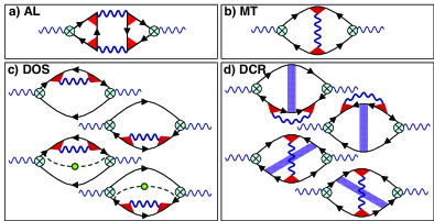
Figure 1: (Color online) Feynman diagrams for the leading-order contributions to the electromagnetic response operator. Wavy lines stand for fluctuation propagators, solid lines with arrows are impurity-averaged normal state Green’s functions, crossed circles are electric field vertices, dashed lines with a circle represent additional impurity renormalizations, and triangles and dotted rectangles are impurity ladders accounting for the electron scattering on impurities (Cooperons).

We start with the derivation of the universal expressions for fluctuation contribution to conductivity and DOS. The electromagnetic response operator in the leading order is defined by ten diagrams LV09 shown in Fig. 1. The corresponding contributions to conductivity at arbitrary magnetic fields and temperatures $T_{\mathrm{c}}\left(H\right)<T\ll\tau^{-1}$ ($\tau$ is the electron elastic scattering time) are:

$$\delta\sigma_{xx}^{\mathrm{AL}} = \frac{e^{2}}{\pi}\sum_{m=0}^{\infty}(m+1)\int_{-\infty}^{\infty}\frac{dx}{\sinh^{2}\pi x}\left\{\frac{\operatorname{Im}^{2}\mathcal{E}_{m}}{\left|\mathcal{E}_{m}\right|^{2}}+\frac{\operatorname{Im}^{2}\mathcal{E}_{m+1}}{\left|\mathcal{E}_{m+1}\right|^{2}}+\frac{\operatorname{Im}^{2}\mathcal{E}_{m+1}-\operatorname{Im}^{2}\mathcal{E}_{m}}{\left|\mathcal{E}_{m}\right|^{2}\left|\mathcal{E}_{m+1}\right|^{2}}\operatorname{Re}\left[\mathcal{E}_{m}\mathcal{E}_{m+1}\right]\right\},$$ (1)

$$\delta\sigma_{xx}^{\mathrm{MT}} = \frac{e^{2}}{\pi}\left(\frac{h}{t}\right)\sum_{m=0}^{M}\underbrace{\frac{{1}}{\gamma_{\phi}+\frac{2h}{t}\left(m+1/2\right)}\int_{-\infty}^{\infty}\frac{dx}{\sinh^{2}\pi x}\frac{\operatorname{Im}^{2}\mathcal{E}_{m}}{\left|\mathcal{E}_{m}\right|^{2}}}_{\delta\sigma_{xx}^{\mathrm{MT(an)}}+\delta\sigma_{xx}^{\mathrm{MT(reg2)}}}+\underbrace{\frac{e^{2}}{\pi^{4}}\left(\frac{h}{t}\right)\sum_{m=0}^{M}\sum_{k=-\infty}^{\infty}\frac{4\mathcal{E}_{m}^{\prime\prime}\left(t,h,|k|\right)}{\mathcal{E}_{m}\left(t,h,|k|\right)}}_{\delta\sigma_{xx}^{\mathrm{MT(reg1)}}},\;$$ (2)

$$\delta\sigma_{xx}^{\mathrm{DOS}} = \frac{2e^{2}}{\pi^{3}}\left(\frac{h}{t}\right)\sum_{m=0}^{M}\int_{-\infty}^{\infty}\frac{dx}{\sinh^{2}\pi x}\frac{\operatorname{Im}\mathcal{E}_{m}\operatorname{Im}\mathcal{E}_{m}^{\prime}}{\left|\mathcal{E}_{m}\right|^{2}},\text{ and}\quad\delta\sigma_{xx}^{\mathrm{DCR}}=\frac{4e^{2}}{3\pi^{6}}\left(\frac{h}{t}\right)^{2}\sum_{m=0}^{M}(m+\frac{1}{2})\sum_{k=-\infty}^{\infty}\frac{8\mathcal{E}_{m}^{\prime\prime\prime}\left(t,h,|k|\right)}{\mathcal{E}_{m}\left(t,h,|k|\right)}.$$ (3)

Here $t=T/T_{\mathrm{c0}},$ $h=\frac{\pi^{2}}{8\gamma_{E}}\frac{H}{H_{\mathrm{c2}}\left(0\right)}=0.69\frac{H}{H_{\mathrm{c2}}\left(0\right)}$, $\gamma_{E}=e^{\gamma_{e}}$ ($\gamma_{e}$ is the Euler constant), $M=\left(tT_{\mathrm{c0}}\tau\right)^{-1},\gamma_{\phi}=\pi/\left(8T_{\mathrm{c0}}\tau_{\phi}\right)$, $\tau_{\phi}$ is the phase-breaking time, $\mathcal{E}_{m}\equiv\mathcal{E}_{m}\left(t,h,ix\right)$ with $\mathcal{E}_{m}\left(t,h,z\right)=\ln t+\psi\left[\frac{1+z}{2}+\frac{2h}{t}\frac{\left(2m+1\right)}{\pi^{2}}\right]-\psi\left(\frac{1}{2}\right)$ and its derivatives $\mathcal{E}_{m}^{(p)}\left(t,h,z\right)\equiv\partial_{z}^{p}\mathcal{E}_{m}\left(t,h,z\right)$. The sum of Eqs. (1)-(3) present the general expression for the total fluctuation correction to conductivity $\delta\sigma_{xx}^{\mathrm{(tot)}}\left(T,H\right)$ that holds in the complete $T$-$H$ phase diagram above the line $H_{c2}(T)$. We analyzed these expressions both analytically (by finding the asymptotic expressions for $\delta\sigma_{xx}^{\mathrm{(tot)}}$ in nine qualitatively different domains) and numerically (by developing a program which calculates the complete surface $\delta\sigma_{xx}^{\mathrm{(tot)}}\left(T,H\right)$ for given parameters $\tau$ and $\tau_{\phi}$) GVVB10 . We show that the singular growth of the conductivity near $T_{\mathrm{c0}}$ transforms into a relatively weak (logarithmic) growth of fluctuation correction to resistivity as one moves along the $H_{\mathrm{c2}}(T)$ line towards the low-temperatures region (i.e. close to $H_{\mathrm{c2}}(0)$). The total fluctuation correction to the conductivity $\delta\sigma^{\mathrm{(tot)}}$ remains negative in a wide domain relatively far from the $H_{\mathrm{c2}}\left(T\right)$ line (see Fig. 2 where the regions with the dominating fluctuation contributions to magneto-conductivity are shown).

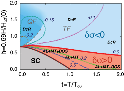
Figure 2: (Color online) Contours of constant fluctuation conductivity [$\delta\sigma=\delta\sigma_{xx}^{\mathrm{(tot)}}\left(t,h\right)$ shown in units of $e^{2}$]. The dominant FC contributions are indicated in bold-italic labels. The dashed line separates the domain of quantum fluctuations (QF) [dark area of $\delta\sigma>0$] and thermal fluctuations (TF). The contour lines are obtained from Eqs. (1)-(3) with $T_{c0}\tau=0.01$ and $T_{c0}\tau_{\phi}=10$.

The analysis of fluctuation corrections enables us to develop a qualitative picture of the quantum phase transition in the vicinity of $H_{\mathrm{c2}}\left(0\right)$. We start by refreshing the well-established qualitative description of the vicinity of $T_{\mathrm{c0}}$. Here the lifetime of fluctuation-induced Cooper pairs (FCP), $\tau_{\mathrm{GL}}$, is obtained using the uncertainty principle: $\tau_{\mathrm{GL}}\sim\hbar/\Delta E$, where $\Delta E$ is the difference $k_{B}(T-T_{\mathrm{c0}})$ ensuring that $\tau_{\mathrm{GL}}$ should become infinite below $T_{\mathrm{c0}}$. This yields the standard Ginzburg-Landau time $\tau_{\mathrm{GL}}\sim\hbar/k_{B}(T-T_{\mathrm{c0}})\sim\hbar/\left(k_{B}T_{\mathrm{c0}}\epsilon\right)$, where $\epsilon=\left(T-T_{\mathrm{c0}}\right)/T_{\mathrm{c0}}\ll 1$ is the reduced temperature. The coherence length $\xi_{\mathrm{GL}}\left(T\right)$ is estimated as the distance which two electrons move apart during the GL time: $\xi_{\mathrm{GL}}\left(\epsilon\right)=\left(\mathcal{D}\tau_{\mathrm{GL}}\right)^{1/2}\sim\xi_{\mathrm{BCS}}/\sqrt{\epsilon}$ ($\xi_{\mathrm{BCS}}$ is the BCS coherence length, $\mathcal{D}$ is the diffusion coefficient). The order parameter $\Delta^{\mathrm{(fl)}}\left(\mathbf{r},t\right)$ varies on the larger scale $\xi_{\mathrm{GL}}\left(T\right)\gg\xi_{\mathrm{BCS}}$. The ratio of the FCP concentration to the corresponding effective mass $n_{\mathrm{c.p.}}/m_{\mathrm{c.p.}}\sim\xi_{\mathrm{GL}}^{2-D}\left(\epsilon\right)$ (with the logarithmic accuracy) in 2D is constant LV09 .

The principal fluctuation contributions to conductivity are positive and originate from direct FCP charge transfer (AL contribution) $\delta\sigma_{xx}^{\mathrm{AL}}\sim\left(n_{\mathrm{c.p.}}/m_{\mathrm{c.p.}}\right)e^{2}\tau_{\mathrm{GL}}\sim e^{2}/\epsilon$ and the specific quantum process of the one-electron charge transfer related to the coherent scattering of electrons on elastic impurities forming FCPs (anomalous MT contribution) $\delta\sigma_{xx}^{\mathrm{MT(an)}}\sim\frac{e^{2}}{\epsilon}\ln\left(\epsilon/\gamma_{\phi}\right)$ LV09 [Fig. 1a,b)]. However, these two contributions do not capture the complete effect of fluctuations on conductivity. The involvement of quasi-particles in the fluctuation pairing results in the opening of the pseudo-gap in the one-electron spectrum. The lack of corresponding electrons at the Fermi level leads to a decrease of the one-electron Drude-like conductivity. Such an indirect fluctuation effect formally is described by the third group of four diagrams in Fig. 1c), which are usually called DOS diagrams. The corresponding contribution has the opposite sign with respect to the AL and MT contributions, but close to $T_{\mathrm{c0}}$ turns to be less singular as a function of temperatureLV09 :

$$\delta\sigma_{xx}^{\mathrm{DOS}}\sim-\frac{2n_{\mathrm{c.p.}}e^{2}\tau}{m_{\mathrm{e}}}\sim-e^{2}\int\frac{\xi_{\mathrm{BCS}}^{2}d^{2}\mathbf{q}}{\epsilon+\xi_{\mathrm{BCS}}^{2}q^{2}}\sim-e^{2}\ln\frac{1}{\epsilon}.$$ (4)

The DOS contribution formally appears due to the summation of  $\left\langle\left|\Delta^{\mathrm{\left(fl\right)}}\left(\mathbf{q},\omega\right)\right|^{2}\right\rangle$ over all long-wave-length fluctuation modes ($q\lesssim\xi_{\mathrm{BCS}}^{-1}\sqrt{\epsilon}$) in the static approximation ($\omega\rightarrow 0$). Relatively far from $T_{\mathrm{c0}}$, $\delta\sigma_{xx}^{\mathrm{DOS}}$ can change the sign of $\delta\sigma_{xx}^{\mathrm{(tot)}}$, but this happens only in the case of strong pair-breaking, when the phase-sensitive anomalous MT contribution is suppressed. Finally, the last four diagrams in Fig. 1d) together with the regular part of the MT diagram describe the renormalization of the diffusion coefficient (DCR) in the presence of fluctuation pairing. Close to $T_{\mathrm{c0}}$ their contribution is not singular, but becomes of primary importance at very low temperatures.

At zero temperature and the field above $H_{\mathrm{c2}}\left(0\right)$, the systematics of the fluctuation contributions to the conductivity considerably changes with respect to that close to $T_{\mathrm{c0}}$. The collisionless rotation of FCPs (they do not “feel” the presence of elastic impurities) results in the lack of their direct contribution to the longitudinal (along the applied electric field) electric transport (analogously to the suppression of one-electron conductivity $\delta\sigma_{xx}^{\left(\mathrm{e}\right)}$ in strong magnetic fields $\omega_{c}\tau\gg 1$, see Ref. A88 ) and the AL contribution to $\delta\sigma_{xx}^{\left(\mathrm{tot}\right)}$ becomes zero. The anomalous MT and DOS contributions turn zero as well but due to different reasons: Namely, the former vanishes since magnetic fields as large as $H_{\mathrm{c2}}\left(0\right)$ completely destroy the phase coherence, whereas the latter disappears since magnetic field suppresses the fluctuation gap in the one-electron spectrum. Therefore the effect of fluctuations on the conductivity at zero temperature is reduced to the renormalization of the one-electron diffusion coefficient. FCPs here occupy the lowest Landau level, but all the dynamic fluctuations in the interval of frequencies from $0$ to $\Delta_{\mathrm{BCS}}$ should be taken into account. The corresponding fluctuation propagator at zero temperature close to $H_{\mathrm{c2}}\left(0\right)$ has the form $L_{0}\left(\omega\right)=N_{0}^{-1}\left(\widetilde{h}+\omega/\Delta_{\mathrm{BCS}}\right)^{-1}$ and

$$\delta\sigma_{xx}^{\mathrm{DCR}}+\delta\sigma_{xx}^{\mathrm{MT(reg)}}\sim-\frac{e^{2}}{\Delta_{\mathrm{BCS}}}\int_{0}^{\Delta_{\mathrm{BCS}}}\frac{d\omega}{\widetilde{h}+\frac{\omega}{\Delta_{\mathrm{BCS}}}}\sim-e^{2}\ln\frac{1}{\widetilde{h}},$$ (5)

where $\widetilde{h}=\left[H-H_{\mathrm{c2}}\left(0\right)\right]/H_{\mathrm{c2}}\left(0\right)$ is the parameter playing the role of the reduced temperature $\epsilon$ in the case of the classical transition; $\Delta_{\mathrm{BCS}}$ is the BCS value of the gap at zero temperature in zero field, and $N_{0}$ is the one-electron density of states.

The microscopic theory provides (unlike the GL approach) a correct description of the short wavelength and high frequency dynamic fluctuations for the complete magnetic field and temperature range. For instance, in the region of QFs, but for non-zero temperatures $t\ll\widetilde{h}$ (see Fig. 2) the AL and the anomalous MT contributions are equal to each other and grow as the square of temperature; moreover, one of them is exactly cancelled by the appearing negative contribution of the four DOS-like diagrams:

$$\delta\sigma_{xx}^{\mathrm{AL}}=\delta\sigma_{xx}^{\mathrm{MT(an)}}=-\delta\sigma_{xx}^{\mathrm{DOS}}=\frac{4e^{2}\gamma_{E}^{2}t^{2}}{3\pi^{2}\widetilde{h}^{2}}.$$ (6)

While Eq. (4) defines the characteristic wavelength $\xi_{\mathrm{GL}}\left(T\right)$ of the fluctuation modes close to $T_{\mathrm{c0}}$, Eq. (5) defines the characteristic coherence time $\tau_{\mathrm{QF}}\left(\widetilde{h}\right)$ of QFs near $H_{\mathrm{c2}}\left(0\right)$ (where $t\ll\widetilde{h}$ ). The integral there is determined by its lower cut off $\omega_{\mathrm{QF}}\sim\Delta_{\mathrm{BCS}}\widetilde{h}$, and the corresponding time scale is $\tau_{\mathrm{QF}}\sim\hbar\left(\Delta_{\mathrm{BCS}}\widetilde{h}\right)^{-1}$. One sees that the functional form of $\tau_{\mathrm{QF}}$ is analogous to that of $\tau_{\mathrm{GL}}$, this can be obtained also from the uncertainty principle. The energy, characterizing the proximity to $H_{\mathrm{c2}}\left(0\right)$, is $\Delta E=\hbar\omega_{c}\left(H\right)-\hbar\omega_{c}\left(H_{\mathrm{c2}}\left(0\right)\right)\sim\Delta_{\mathrm{BCS}}\widetilde{h}$ in this case. However, the spatial scale of QFs close to $H_{\mathrm{c2}}\left(0\right)$ cannot be found from the propagator describing QFs, since the latter in the Landau representation does not contain space variables. Nevertheless, the spatial coherence scale can be estimated from the value of $\tau_{\mathrm{QF}}$ analogously to consideration near $T_{\mathrm{c0}}$. Namely, two electrons with the coherent phase starting from the same point get separated by the distance $\xi_{\mathrm{QF}}\sim\left(\emph{D}\tau_{\mathrm{QF}}\right)^{1/2}\sim\xi_{\mathrm{BCS}}/\sqrt{\widetilde{h}}$ after the time $\tau_{\mathrm{QF}}$. During this time they participate in multiple fluctuating Cooper pairings maintaining their coherence.

To clarify the physical meaning of $\tau_{\mathrm{QF}}$ and $\xi_{\mathrm{QF}}$, note that near the quantum phase transition at zero temperature, where $H\rightarrow H_{\mathrm{c2}}\left(0\right)$, the fluctuations of the order parameter $\Delta^{\mathrm{(fl)}}\left(\mathbf{r},t\right)$ become highly inhomogeneous, contrary to the situation near $T_{\mathrm{c0}}$. Indeed, below $H_{\mathrm{c2}}\left(0\right)$, the spatial distribution of the order parameter at finite magnetic field reflects the existence of Abrikosov vortices with average spacing (close to $H_{\mathrm{c2}}\left(0\right)$ but in the region where the notion of vortices is still adequate) equal to $\xi_{\mathrm{BCS}}/\sqrt{H_{\mathrm{c2}}\left(0\right)/H}$. Therefore, one expects that close to and above $H_{\mathrm{c2}}\left(0\right)$ the fluctuation order parameter also varies over the scale of $\xi_{\mathrm{BCS}}$. At fields higher but not too far from $H_{\mathrm{c2}}\left(0\right)$ one can expect that these “vortex-like” spatial inhomogeneities are preserved over the time scale $\tau_{\mathrm{QF}}$, whereas $\Delta^{\mathrm{(fl)}}\left(\mathbf{r},t\right)$ varies over the spatial scale $\xi_{\mathrm{BCS}}$. The coherence length $\xi_{\mathrm{QF}}$ is thus a characteristic size of a cluster of coherently rotating FCPs, and $\tau_{\mathrm{QF}}$ estimates the lifetime of such flickering clusters.

In terms of these introduced QF characteristics $\tau_{\mathrm{QF}}$ and $\xi_{\mathrm{QF}}$ one can understand the meaning of already found microscopic QF contributions and derive others which are required. For example, the physical meaning of Eq. (6) can be understood as follows: one could estimate the FCP conductivity by mere replacing $\tau_{\mathrm{GL}}\rightarrow\tau_{\mathrm{QF}}$ in the classical AL formula, which would give $\delta\widetilde{\sigma}^{AL}\sim e^{2}\tau_{\mathrm{QF}}.$ Nevertheless, as we already noticed, the FCPs at zero temperature cannot move in the electric field but only rotate. As temperature deviates from zero, the FCP can change their state due to the interaction with the thermal bath, i.e. their hopping to an adjacent rotation trajectory along the applied electric field becomes possible. This means that they can participate in longitudinal charge transfer. This process can be mapped onto the paraconductivity of a granular superconductors LVV08 at temperatures above $T_{\mathrm{c0}}$, where the FCP tunnelling between grains occurs in two steps: first one electron jumps, then the second follows. The probability of each hopping event is proportional to the inter-grain tunneling rate $\Gamma.$ To conserve the superconductive coherence between both events, the latter should occur during the FCP lifetime $\tau_{\mathrm{GL}}.$ The probability of FCP tunnelling between two grains is determined as the conditional probability of two one-electron hopping events and is proportional to $W_{\Gamma}=\Gamma^{2}$ $\tau_{\mathrm{GL}}.$  Coming back to the situation of FCPs above $H_{\mathrm{c2}}\left(0\right)$, one can identify the tunnelling rate with temperature $T$ while $\tau_{\mathrm{GL}}$ corresponds to $\tau_{\mathrm{QF}}.$ Therefore, in order to get a final expression, $\delta\widetilde{\sigma}^{\mathrm{AL}}$ should be multiplied by the probability factor $W_{\mathrm{QF}}=t^{2}\tau_{\mathrm{QF}}$ of the FCP hopping to the neighboring trajectory: $\delta\sigma_{xx}^{\mathrm{AL}}\sim\delta\widetilde{\sigma}^{AL}W_{\mathrm{QF}}\sim e^{2}t^{2}/\widetilde{h}^{2},$ which corresponds to the low temperature asymptotic Eq. (6).

The total fluctuation contribution to conductivity $\delta\sigma_{xx}^{\left(\mathrm{tot}\right)}$ at $t\ll\widetilde{h}$ turns out to be negative and diverges logarithmically when the magnetic field approaches $H_{c2}\left(0\right):$

$$\delta\sigma_{xx}^{\mathrm{tot}}=-\frac{2e^{2}}{3\pi^{2}}\ln\frac{1}{\widetilde{h}}-\frac{6\gamma_{E}e^{2}}{\pi^{2}}\frac{t}{\widetilde{h}}+O\left[\left(\frac{t}{\widetilde{h}}\right)^{2}\right].$$ (7)

The numerical analysis of Eqs. (1)-(3) shows that the asymptotic Eq. (7) is valid only within the narrow field range $\widetilde{h}\lesssim 10^{-6}$. The nontrivial fact following from Eqs. (1)-(3) is that an increase of temperature at a fixed value of the magnetic field in this domain results in a non-monotonic behavior of the fluctuation part of the conductivity GL01 (see Fig. 2), observed in experiments Bridgitte ; Batur .

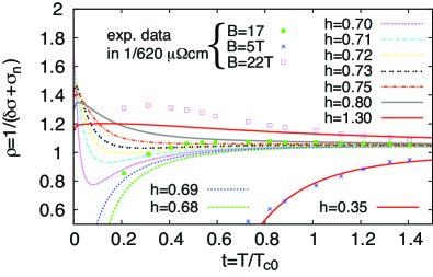
Figure 3: (Color online) Temperature dependence of the FC at different fields close to $H_{c2}(0)$ and comparison to experimental data for thin films of La_2-xSr_xCuO₄ with $T_{c0}\approx 19$K and $B_{c2}(0)\approx 15$T.  Note, that for the theoretical curves a fixed $T_{c0}\tau_{\phi}=10$ is used which does not necessarily agree with the experimental value. Nevertheless, the overall behavior can be captured by this rough comparison. All curves are numerically calculated with $T_{c0}\tau=0.01$.

Now we estimate the contributions of QFs to different characteristics of the SC in the vicinity of $H_{\mathrm{c2}}\left(0\right)$. Applying the Langevin formula $\chi=e^{2}\left(n/mc\right)\left\langle R^{2}\right\rangle$ to a coherent cluster and taking $n_{\mathrm{c.p}.}/m_{\mathrm{c.p}.}\sim 1$, $R^{2}\sim\xi_{\mathrm{QF}}^{2}\left(\widetilde{h}\right)$ one finds the fluctuation magnetic susceptibility $\chi^{\mathrm{AL}}\sim\xi_{\mathrm{BCS}}^{2}/c\widetilde{h}$ in an agreement with Ref. GL01 . One further reproduces the contribution of QF to the Nernst coefficient SSVG09 . Using $\nu\sim\left[\sigma/\left(ne^{2}c\right)\right]d\mu/dT$ and identifying the chemical potential of FCP, $\mu_{\mathrm{FCP}}$, as $\hbar\omega_{\mathrm{c}}\left(H_{\mathrm{c2}}\left(0\right)\right)-\hbar\omega_{\mathrm{c}}\left(H\right)$ (as in Ref. SSVG09 , close to $T_{\mathrm{c0}}$, $\mu_{\mathrm{FCP}}=T_{\mathrm{c0}}-T$), one finds that $d\mu_{\mathrm{FCP}}/dT\sim dH_{\mathrm{c2}}\left(T\right)/dT\sim-T/\Delta_{\mathrm{BCS}}$ and $\nu^{\mathrm{AL}}\sim\xi_{\mathrm{BCS}}^{2}t/\widetilde{h}$. One can also predict the non-monotonic dependence of the transverse fluctuation conductivity $\delta\sigma_{zz}^{\left(\mathrm{tot}\right)}\left(\widetilde{h},0\right)$ above $H_{\mathrm{c2}}\left(0\right)$ for layered SCs in a field perpendicular to the layers. The motion of FCPs along the z-axis has hopping character, and applying the above mapping procedure one finds: $\delta\sigma_{zz}^{\mathrm{AL}}\left(\widetilde{h},0\right)\sim\delta\widetilde{\sigma}^{\mathrm{AL}}\Gamma^{2}$ $\tau_{\mathrm{QF}}=e^{2}\Gamma^{2}/\widetilde{h}^{2}$. The same holds for the quasi-particle contributions (accounting for the anisotropy factor BDKLV93 ), and $\delta\sigma_{zz}^{\mathrm{DOS}}\sim-\left(\Gamma/E_{\mathrm{F}}\right)e^{2}\ln\left(1/\widetilde{h}\right)$. As a result $\delta\sigma_{zz}^{\mathrm{tot}}\sim e^{2}\Gamma^{2}/\widetilde{h}^{2}-\left(\Gamma/E_{\mathrm{F}}\right)e^{2}\ln\left(1/\widetilde{h}\right)$ explaining the strong growth of the transversal magneto-resistance in organic superconductors at the edge of the transition at very low temperatures MK10 .

Finally, our results can be used for the analysis of novel studies of superconductors in ultra-high magnetic fields Bridgitte (see also Fig. 2), for the separation of quantum corrections in the vicinity of the superconductor–insulator transition Batur , and the precise definition of the critical temperature and extraction of the temperature dependence of $\tau_{\phi}\left(T,H\right)$.

We thank Yu. Galperin, M.  Kartsovnik, A. Koshelev, M. Norman, and T.  Baturina for useful discussions. The work was supported by the U.S. Department of Energy Office of Science under the Contract No. DE-AC02-06CH11357. A.A.V. acknowledges support of the MIUR under the project PRIN 2008.

References

• (1) A.I. Larkin, A.A. Varlamov, Theory of Fluctuations in Superconductors, OUP, Second Edition, (2009).
• (2) L.G. Aslamazov, and A.I. Larkin,  Soviet Solid State Physics, 10, 875 (1968).
• (3) K. Maki. Progress in Theoretical Physics, 39, 897; ibid. 40, 193 (1968).
• (4) R.S. Thompson, Physical Review B1, 327 (1970).
• (5) L.B. Ioffe, A.I. Larkin, A.A. Varlamov, Yu. Lu, Phys. Rev. B47, 8936 (1993);
• (6) V.V. Dorin, R.A. Klemm, A.A. Varlamov, A.I. Buzdin, D.V. Livanov, Phys. Rev. B48, 12591 (1993).
• (7) L.G. Aslamazov, and A.A. Varlamov,  Journal of Low Temp. Phys., 38, 223 (1980).
• (8) A.I. Larkin, JETP Letters, 31, 219 (1980).
• (9) B.L. Altshuler, M.Yu. Reyzer, A.A. Varlamov, Soviet JETP, 57, 1329 (1983).
• (10) J.M.B. Lopes dos Santos, E. Abrahams, Physical Review, B31, 172 (1985).
• (11) V. Galitski, A.I. Larkin, Phys. Rev. 95, 107005 (2001).
• (12) I.S. Beloborodov, K.B. Efetov, and A.I. Larkin, Physical Review, B61, 9145 (2000).
• (13) M.A. Skvortsov, M. Serbin, A.A. Varlamov, V. Galitski, Phys. Rev. Lett., 102, 067001, (2009).
• (14) Andreas Glatz, A.A. Varlamov, V.M. Vinokur, T.I. Baturina, to be published.
• (15) A.A. Abrikosov Fundamentals of Metal Theory, Elseivir, (1988).
• (16) I.V. Lerner, A. A. Varlamov, V. M. Vinokur, Phys. Rev. Lett., 100, 117003, (2008).
• (17) M. Kartsovnik, private communication.
• (18) B. Leridon, J. Vanacken, T. Wambecq, and V. Moshchalkov, Phys. Rev. B 76, 012503 (2007).
• (19) V.F. Gantmakher et al., JETP Letters, 77, 498 (2003).