An update on the double cascade scenario in two-dimensional turbulence

Abstract

Statistical features of homogeneous, isotropic, two-dimensional turbulence is discussed on the basis of a set of direct numerical simulations up to the unprecedented resolution $32768^{2}$. By forcing the system at intermediate scales, narrow but clear inertial ranges develop both for the inverse and for direct cascades where the two Kolmogorov laws for structure functions are, for the first time, simultaneously observed. The inverse cascade spectrum is found to be consistent with Kolmogorov-Kraichnan prediction and is robust with respect the presence of an enstrophy flux. The direct cascade is found to be more sensible to finite size effects: the exponent of the spectrum has a correction with respect theoretical prediction which vanishes by increasing the resolution.

“Now, listen to me. You are living on a Plane. What you style Flatland is the vast level surface of what I may call a fluid on, or in, the top of which you and your countrymen move about, without rising above it or falling below it.”
Flatland by E.A. Abbott

The existence of two quadratic inviscid invariants is the most distinguishing feature of Navier Stokes equations in two dimensions. On this basis, R.H. Kraichnan Kraichnan (1967) predicted many years ago the double cascade scenario: when the turbulent flow is sustained by an external forcing acting on a typical scale $\ell_{f}$, an inverse cascade of kinetic energy $E=1/2\langle v^{2}\rangle$ to large scales ($\ell\gg\ell_{f}$) and a direct cascade of enstrophy $Z=1/2\langle\omega^{2}\rangle$ to small scales ($\ell\ll\ell_{f}$) develop. In inverse and direct ranges of scales the theory predicts the kinetic energy spectrum $E(k)\simeq\varepsilon^{2/3}k^{-5/3}$ and $E(k)\simeq\eta^{2/3}k^{-3}$ with possible logarithmic corrections (Kraichnan (1971)). Here $\varepsilon$ and $\eta\simeq k_{f}^{2}\varepsilon$ are respectively the energy and the enstrophy injection rate.

Navier-Stokes equations in two dimensions are now the prototypical model for turbulent systems displaying a double cascade scenario. From two-dimensional magneto-hydro-dynamics, to many geophysical model (such as Charney-Hasegawa-Mima), to wave turbulence models, the picture originally developed by Kraichnan has found many fruitful applications.

Despite the expansion of the fields of applicability, it is remarkable that the verification of Kraichnan’s theory, after more than $40$ years from its formulation, is still partial. This is due to several reasons. First of all, the difficulties to generate a laboratory flow which is truly two dimensional on a large range of scales, limits the experimental approaches. From a numerical point of view, the situation in two dimensions is apparently very convenient with respect to three dimensions. A deeper analysis shows that this is not the case, as the simultaneous simulation of two inertial ranges requires very large resolutions. Moreover, because time step is proportional to grid size, the computational effort for simulating two-dimensional turbulence can be even larger than in the three dimensional case.

In the present paper we report numerical results on the statistics of the two cascades of two-dimensional turbulence on the basis of very high resolution (up to $32768^{2}$) direct numerical simulations. Together with previous results at lower resolutions (already reported on Boffetta (2007)) we obtain strong indications that the classical Kraichnan scenario is recovered in the limit of two infinitely extended inertial ranges, although we are unable to address the issue of possible logarithmic corrections in the direct cascade.

The motion of an incompressible (${\bf\nabla}\cdot{\bf u}=0$) fluid in two dimensions is governed by the Navier–Stokes equations which are written for the scalar vorticity field $\omega={\bf\nabla}\times{\bf u}$ as

$$\partial_{t}\omega+{\bf u}\cdot{\bf\nabla}\omega=\nu\nabla^{2}\omega-\alpha\omega+f_{\omega}\,.$$ (1)

In (1) $\nu$ is the kinematic viscosity, $f_{\omega}$ is a forcing term and the friction term $-\alpha\omega$ removes energy at large scales in order to reach a stationary state. Alternatively, one can consider the quasi-stationary regime with $\alpha=0$ in which the integral scale grows, according to Kolmogorov scaling, as $L(t)=\varepsilon^{1/2}t^{3/2}$. In this case, Galilean invariant statistics (i.e. velocity structure functions or energy spectrum) is stationary at small scales $\ell<L(t)$. We remark that the form of the friction term in (1) physically represents a crude approximation of the effects induced by bottom or air friction on a thin layer of fluid Clercx and van Heijst (2009).

We numerically integrate (1) by means of a standard, fully dealiased, pseudo-spectral parallel code on a double periodic square domain of side $L_{x}=L_{y}=2\pi$ at spatial resolution up to $N=32768$. The forcing term $f_{\omega}$ in (1) is $\delta$-correlated in time (in order to control energy and enstrophy input) and peaked on a characteristic forcing scale $\ell_{f}$. We use either a Gaussian forcing with correlation function $\langle f_{\omega}({\bf r},t)f_{\omega}({\bf 0},0)\rangle=F\delta(t)\exp(-(r/\ell_{f})^{2})$ or a forcing which has support on a narrow band of wavenumbers around $k_{f}=\pi/\ell_{f}$ in Fourier space. In both cases this ensures that energy and enstrophy input are localized in Fourier space and only a limited range of scales around the forcing scale is affected by the details of the forcing statistics. More complex forcing, not localized in wavenumber space, can have a direct effect on inertial range scales Mazzino et al. (2007); Clercx and van Heijst (2009). The forcing scale in all run is fixed at $\ell_{f}=L_{x}/100$ to allow the development of inertial ranges both at scales $\ell>\ell_{f}$ (inverse cascade) and $\ell<\ell_{f}$ (direct cascade). For the largest simulation run ($N=32768$) we study the inverse cascade in the quasistationary regime with $\alpha=0$ and we stop the integration of (1) when $L(t)<L_{x}$ to avoid the pile-up of energy at the largest available scale. Table 1 reports the most important parameters for the simulations.

Label	A	B	C	D	E
N	$2048$	$4096$	$8192$	$16384$	$32768$
$\nu$	$2\times 10^{-5}$	$5\times 10^{-6}$	$2\times 10^{-6}$	$1\times 10^{-6}$	$2.5\times 10^{-7}$
$\alpha$	$0.015$	$0.024$	$0.025$	$0.03$	$0.0$
$\ell_{f}/\ell_{\nu}$	$13$	$26$	$40$	$57$	$116$
$R_{\lambda}$	$7.9$	$15.4$	$21.5$	$26.0$	$36.0$
$\varepsilon_{\alpha}/\varepsilon_{I}$	$0.54$	$0.83$	$0.92$	$0.95$	$0.98$
$\eta_{\nu}/\eta_{I}$	$0.96$	$0.92$	$0.90$	$0.88$	$0.98$
$\delta$	$1.8$	$1.1$	$0.75$	$0.50$	$0.35$

Table 1: Parameters of the simulations. $N$ spatial resolution, $\nu$ viscosity, $\alpha$ friction, $\ell_{f}=\pi/k_{f}$ forcing scale, $R_{\lambda}=Z^{3/2}/\eta_{\nu}$ Reynolds number for the direct cascade Herring et al. (1974), $\ell_{\nu}=\nu^{1/2}/\eta_{\nu}^{1/6}$ enstrophy dissipative scale, $\varepsilon_{I}$ energy injection rate, $\varepsilon_{\alpha}$ friction energy dissipation rate (large-scale energy flux for run E), $\eta_{I}$ enstrophy injection rate, $\eta_{\nu}$ viscous enstrophy dissipation rate, $\delta$ correction to the Kraichnan spectral exponent in the direct cascade. Viscosity is tuned to have for all runs $k_{max}\ell_{\nu}\simeq 3$. For the run $E$, for which $\alpha=0$, $\varepsilon_{\alpha}$ is kinetic energy growth rate.

The first information we get from the Table is related to the direction of the energy and enstrophy fluxes. According to the original idea of Kraichnan on the double cascade, in the ideal case of an infinite inertial range all the energy (enstrophy) injected should be transferred to large (small) scales. This can be thought as a limit case of a realistic situation in which the inertial range has a finite extension because of the presence of large and small scale dissipation. The characteristic viscous scale $\ell_{\nu}$ and friction scale $\ell_{\alpha}$ can be expressed in terms of the energy (enstrophy) viscous dissipation rate $\varepsilon_{\nu}$ ($\eta_{\nu}$) and friction dissipation rate $\varepsilon_{\alpha}$ ($\eta_{\alpha}$) by the relations $\ell_{\nu}^{2}=\varepsilon_{\nu}/\eta_{\nu}$ and $\ell_{\alpha}^{2}=\varepsilon_{\alpha}/\eta_{\alpha}$. Energy and enstrophy balance equations in stationary conditions give Kraichnan (1967); Borue (1993); Eyink (1995)

$${\varepsilon_{\nu}\over\varepsilon_{\alpha}} = \left({\ell_{\nu}\over\ell_{f}}\right)^{2}\left({\ell_{f}\over\ell_{\alpha}}\right)^{2}{(\ell_{\alpha}/\ell_{f})^{2}-1\over 1-(\ell_{\nu}/\ell_{f})^{2}}$$ (2)

$${\eta_{\nu}\over\eta_{\alpha}} = {(\ell_{\alpha}/\ell_{f})^{2}-1\over 1-(\ell_{\nu}/\ell_{f})^{2}}$$ (3)

Therefore with an extended direct inertial range, $\ell_{\nu}\ll\ell_{f}$, one has $\varepsilon_{\nu}/\varepsilon_{\alpha}\to 0$, i.e. all the energy injected goes to large scales. Moreover, if $\ell_{\alpha}\gg\ell_{f}$ one obtains $\eta_{\alpha}/\eta_{\nu}\to 0$ i.e. all the enstrophy goes to small scales to generate the direct cascade. Indeed, from Table 1 we see that increasing the resolution, i.e. $\ell_{f}/\ell_{\nu}$, the fraction of energy which flows to large scales increases. Because in our runs $\ell_{\alpha}/\ell_{f}$ is constant with resolution and because $\ell_{\nu}\propto\nu^{1/2}$ we expect that, according to (2), $\varepsilon_{\nu}/\varepsilon_{\alpha}\propto\nu$ Kraichnan (1967) as indeed is shown in the inset of Fig. 1.

Most of the enstrophy (around $90\%$) is dissipated by small scale viscosity. We observe a moderate increase of the large-scale contribution to enstrophy dissipation $\eta_{\alpha}$ by going from run $A$ to $D$. This is a finite size effect because we have to increase the friction coefficient $\alpha$ with the resolution $N$ in order to keep the friction scale $\ell_{\alpha}\simeq\alpha^{-3/2}\varepsilon_{\alpha}^{1/2}$ constant when $\varepsilon_{\alpha}$ grows. Indeed, for the run $E$ without large-scale friction, the enstrophy flux to small scales almost balances the input.

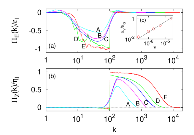
Figure 1: (Color online). (a) Energy and (b) enstrophy fluxes in Fourier space for the runs of Table 1. Fluxes for runs $D$ and $E$ are computed from a single snapshot. Inset (c): ratio of viscous over friction energy dissipation versus kinematic viscosity for the $5$ runs, the line represents a linear fit.

Figure 1 shows the energy and enstrophy fluxes in Fourier space defined as $\Pi_{E}(k)\equiv-\partial_{t}\int_{0}^{k}E(k^{\prime})dk^{\prime}$ and $\Pi_{Z}(k)\equiv-\partial_{t}\int_{0}^{k}k^{\prime 2}E(k^{\prime})dk^{\prime}$ (where $E(k)$ is the energy spectrum and the time derivative keeps the contribution from nonlinear terms in (1) only Frisch (1995)). We observe that, because resolution is changed by keeping $\ell_{\alpha}\gg\ell_{f}$ constant, the only effect of increasing resolution on the inverse cascade is the growth of $\varepsilon_{\alpha}/\varepsilon_{I}$ (i.e. $\Pi_{E}(k)/\varepsilon_{I}$) as discussed above, while the extension of the inertial range does not change. Despite the limited resolution of the inverse cascade inertial range ($k_{f}=100$), we observe an almost constant energy flux which develops independently on the presence of a direct cascade inertial range (run A). Of course, because of the presence of the two energy sinks (viscosity and friction) a plateau indicating a constant energy flux is clearly observable for the largest resolution simulation $E$ only. On the contrary, the direct cascade does not develop for the small resolution runs as the dissipative scale is very close to the forcing scale (see Table 1). A constant enstrophy flux $\Pi_{Z}(k)$ which extends over about one decade is on the other hand obtained for the most resolved run $E$.

The behavior of the fluxes around $k\simeq k_{f}$ depends on the details of the injection: transition from zero to negative (positive) energy (enstrophy) flux is sharp in the case of forcing on a narrow band of wavenumber (run D and E) while it is more smooth for the Gaussian forcing which is active on more scales.

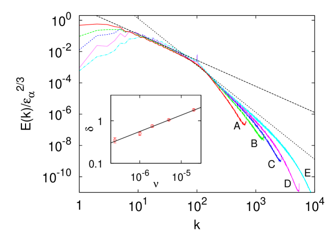
Figure 2: (Color online). Energy spectra for the simulation of Table 1 compensated with the inverse energy flux. Lines represent the two Kraichnan spectra $Ck^{-5/3}$ (dashed) with $C=6$ and $k^{-3}$ (dotted). The inset shows the correction $\delta$ to the Kraichnan exponent for the direct cascade $3$ obtained from the minimum of the local slope of the spectra in the range $k_{f}\leq k\leq k_{\nu}$ as a function of the viscosity. Errorbars are obtained from the fluctuations of the local slope. The line has a slope $0.38$ and is a guide for the eye.

In Fig. 2 we plot the energy spectra of the different runs compensated with the energy flux. In the inverse range $k<k_{f}$ a Kolmogorov spectrum $E(k)=C\varepsilon_{\alpha}^{2/3}k^{-5/3}$ is clearly observed for all simulations. The value of the Kolmogorov constant $C\simeq 6$ is compatible with those obtained from more resolved inertial range Boffetta et al. (2000) and it is found to be independent on the resolution. For what concerns the direct cascade, the spectrum is steeper than the Kraichnan prediction $k^{-3}$. This effect is due to finite size effects, as it reduces by increasing the resolution. In order to quantify the recovery of the Kraichnan exponent, we computed for all runs the local slope of the energy spectra in the range of wavenumber $k_{f}\leq k\leq k_{\nu}$. A plateau for the slope in this range of scales defines the scaling exponent $-(3+\delta)$ of the energy spectrum in the direct cascade. In the inset of Fig. 2 we plot the measured value of the correction $\delta$ as a function of the viscosity of the run. It is evident that, despite the fact the classical exponent $-3$ is not observed, the indication is that it should eventually be recovered in the infinite resolution limit $\nu\to 0$. It is interesting to observe that for the most resolved run $E$, for which the enstrophy flux is almost constant over a decade of wavenumbers (see Fig. 1), the exponent of the energy spectrum still has a significant correction $\delta\simeq 0.35$. We remark that a clear observation of Kraichnan $k^{-3}$ spectrum in simulations is obtained using some kind of modified viscosity only Borue (1993); Lindborg and Alvelius (2000); Pasquero and Falkovich (2002), while steeper spectra has also been observed in simulations of (1) with a large scale forcing, i.e. resolving the direct cascade only Gotoh (1998). Therefore also for the direct cascade our simulations support the picture for which the statistics of one cascade is independent on the presence of the other cascade.

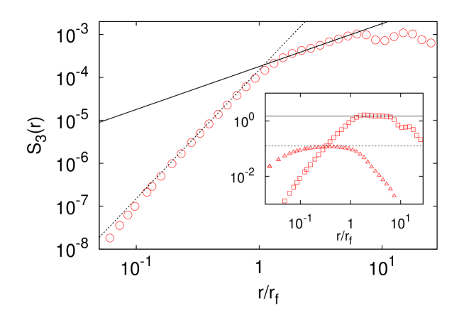
Figure 3: (Color online). Third-order longitudinal velocity structure function $S_{3}(r)\equiv\langle(\delta u_{\parallel}(r))^{3}\rangle$ for run $E$ at final time. The two lines represent the Kolmogorov laws (4) (continuous) and (5) (dotted). Inset: compensation of $S_{3}(r)$ with $\varepsilon_{\alpha}r$ (circles) and with $\eta_{\nu}r^{3}$ (triangles). Lines are the coefficient $3/2$ (continuous) and $1/8$ (dotted).

We now consider small scale statistics in physical space, starting from velocity structure function $S_{p}(r)\equiv\langle(\delta u_{\parallel}(r))^{p}\rangle$ (with $(\delta u_{\parallel}(r)=({\bf u}({\bf x}+{\bf r})-{\bf u}({\bf x}))\cdot{\bf r}/r$). The Kolmogorov relation, a consequence of constant energy (or enstrophy) flux in the inertial range, together with assumptions of homogeneity and isotropy, gives an exact prediction for the third-order longitudinal velocity structure function $S_{3}(r)$ Bernard (1999); Lindborg (1999); Yakhot (1999). For the inverse cascade it predicts

$$S_{3}(r)={3\over 2}\varepsilon_{\alpha}r\;\;\;\;\mbox{for}\;\;\;\;r\gg\ell_{f}$$ (4)

while for the direct cascade

$$S_{3}(r)={1\over 8}\eta_{\nu}r^{3}\;\;\;\;\mbox{for}\;\;\;\;r\ll\ell_{f}$$ (5)

The third-order velocity structure function for the simulation $E$ is shown in Fig. 3. Both Kolmogorov laws are clearly visible with the predicted coefficients. We remark that this is the first time that the two fundamental laws (4) and (5) are observed simultaneously.

In Fig. 4 we plot velocity structure functions of different orders together with the compensation with Kolmogorov scaling $S_{p}(r)\simeq(\varepsilon_{\alpha}r)^{p/3}$. Although the range of scaling is very small, the presence of a plateau in the inverse cascade range of scales confirms that intermittency corrections are very small or absent in the inverse cascade range Boffetta et al. (2000).

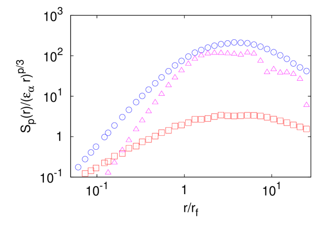
Figure 4: (Color online). Longitudinal velocity structure function $S_{p}(r)$ of order $p=2$ (red squares), $p=4$ (blue circles) and $p=5$ (pink triangles) from run $E$ and compensated with Kolmogorov-Kraichnan prediction $(\varepsilon_{\alpha}r)^{p/3}$.

Velocity structure functions are trivially dominated by the IR contribution in the direct cascade range. Therefore to investigate higher order statistics of the direct cascade one has consider either increments of velocity derivatives (e.g. vorticity increments) or velocity second-differences (the latter having the advantage of being Reynolds-number-independent in the limit of zero viscosity). A Kraichnan energy spectrum $k^{-3}$ would correspond dimensionally to flat vorticity structure functions, and indeed zero scaling exponents for $p>3$ Eyink (1996) or logarithmic structure functions Falkovich and Lebedev (1994) are predicted in the limit of vanishing viscosity. Power-law intermittency corrections in the direct cascade of Navier-Stokes equations are excluded by theory (while logarithmic corrections are in principle possible), but it is known that the presence of a linear friction terms in (1) can both steepen the spectrum and generate intermittency Nam et al. (2000); Bernard (2000); Boffetta et al. (2002).

We have seen that in our simulations, even at highest resolution and without friction, we observe a correction to the spectral exponent, and therefore we cannot expect to observe theoretically predicted vorticity structure functions. Moreover, because of the limited resolution of the direct cascade, no clear scaling in vorticity structure functions is observed. Nonetheless we can address the issue of intermittency by looking at the probability density functions of fluctuations of vorticity at different scales within the inertial range. The result, for run $E$ is shown in Fig. 5 for both velocity and vorticity increments. For what concerns $\delta u_{\parallel}(r)$ we observe self-similar pdf in the inertial range of scales, in agreement with the normal scaling of Fig. 4. The shape of pdf is very close to Gaussian with a flatness which is around $3.3$. On the contrary, vorticity increments $\delta\omega(r)$ are definitely far from Gaussian with tails which are found to be very close to exponentials. Nonetheless, the shape of the pdf does not change substantially in the range of scale of the direct cascade, an indication of small intermittency also in this case.

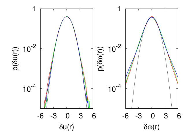
Figure 5: (Color online). Probability density functions (pdf) of velocity longitudinal increments $\delta u_{\parallel}(r)$ at scales $r=2.5\ell_{f}$ (red outer line) $r=5.0\ell_{f}$ (green middle line) and $r=10.0\ell_{f}$ (blue inner line) rescaled with rms values (left panel). Pdf of vorticity increments $\delta\omega(r)$ at scales $r=0.2\ell_{f}$ (red inner line) $r=0.4\ell_{f}$ (green middle line) and $r=0.8\ell_{f}$ (blue outer line) rescaled with rms values (right panel). Black curves are standard Gaussian. Data from run $E$.

Velocity increments pdf in Fig. 5 cannot be exactly Gaussian as the energy flux, proportional to $S_{3}(r)$, requires a positive skewness. Energy and enstrophy fluxes are defined in physical space in terms of filtered fields, as described in Chen et al. (2003, 2006). We introduce a large scale vorticity field $\omega_{r}\equiv G_{r}\star\omega$ and a large scale velocity field ${\bf u}_{r}\equiv G_{r}\star{\bf u}$ obtained from convolution with a Gaussian filter $G_{r}(\bf x)$. From those fields, energy and enstrophy fluxes $\Pi_{r}^{(E,Z)}({\bf x},t)$, representing the local transfer of energy/enstrophy from scales larger than $r$ to scales smaller to $r$, are defined as

$$\Pi_{r}^{(E)}({\bf x},t)\equiv-(\tau_{\alpha\beta})_{r}\nabla_{\alpha}(v_{\beta})_{r}$$ (6)

$$\Pi_{r}^{(Z)}({\bf x},t)\equiv-(\sigma_{\alpha})_{r}\nabla_{\alpha}\omega_{r}$$ (7)

where $(\tau_{\alpha\beta})_{r}=(v_{\alpha}v_{\beta})_{r}-(v_{\alpha})_{r}(v_{\beta})_{r}$ and $(\sigma_{\alpha})_{r}=(v_{\alpha}\omega)_{r}-(v_{\alpha})_{r}\omega_{r}$.

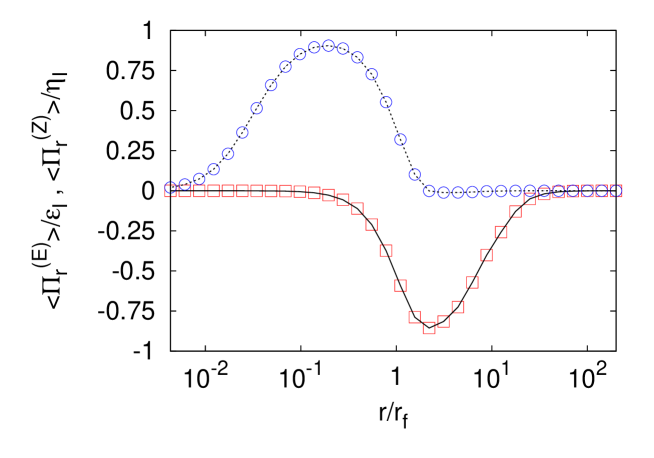
Figure 6: (Color online). Average energy (lower line, red squares) and enstrophy (upper line, blue circles) fluxes in physical space for run $E$ normalized with energy/enstrophy inputs.

Figure 6 shows the physical fluxes averaged over space at final time of simulation $E$. The two range of scales for the energy and enstrophy cascades are evident for $r/\ell_{f}>1$ and $r/\ell_{f}<1$ respectively. The finite mean values of fluxes are the results of strong cancellation: the ratio between the (absolute) mean value and the standard deviation at the scales $r_{1}\simeq 2.2\ell_{f}$ and $r_{2}\simeq 0.19\ell_{f}$ corresponding to the peaks of the two fluxes are $-0.19$ and $0.16$ for energy and enstrophy respectively. The correlation among the two fluxes is small: the correlation coefficient between $\Pi_{r_{1}}^{(E)}$ and $\Pi_{r_{2}}^{(Z)}$ is only $C(r_{1},r_{2})\simeq-0.17$ confirming the picture of independence of the fluxes in physical spaces already observed at lower resolution Boffetta (2007).

In conclusion, on the basis of very high resolution numerical simulations, we obtain strong evidence that the double cascade theory developed by Kraichnan more than 40 years ago is substantially correct. This result required massive resolution as two inertial ranges have to be resolved simultaneously. It is worth remarking that, despite some effort Rutgers (1998); Bruneau and Kellay (2005), the clear observation of the two cascade is still lacking in experiments. We hope that our results will stimulate further experimental investigations of the double cascade scenario.

Numerical simulations has been performed within the DEISA Extreme Computing Initiative program “Turbo2D”.

References

- Kraichnan (1967) R. Kraichnan, Phys. Fluids 10, 1417 (1967).
- Kraichnan (1971) R. Kraichnan, J. Fluid Mech. 47, 525 (1971).
- Boffetta (2007) G. Boffetta, J. Fluid Mech. 589, 253 (2007).
- Clercx and van Heijst (2009) H. J. H. Clercx and G. J. F. van Heijst, Applied Mechanics Reviews 62 (2009).
- Mazzino et al. (2007) A. Mazzino, P. Muratore-Ginanneschi, and S. Musacchio, Phys. Rev. Lett. 99, 144502 (2007).
- Herring et al. (1974) J. Herring, S. Orszag, R. Kraichnan, and D. Fox, J. Fluid Mech. 66, 417 (1974).
- Borue (1993) V. Borue, Phys. Rev. Lett. 71, 3967 (1993).
- Eyink (1995) G. L. Eyink, Phys. Rev. Lett. 74, 3800 (1995).
- Frisch (1995) U. Frisch, Turbulence: The Legacy of AN Kolmogorov (Cambridge University Press, Cambridge, 1995).
- Boffetta et al. (2000) G. Boffetta, A. Celani, and M. Vergassola, Phys. Rev. E 61, R29 (2000).
- Lindborg and Alvelius (2000) E. Lindborg and K. Alvelius, Phys. Fluids 12, 945 (2000).
- Pasquero and Falkovich (2002) C. Pasquero and G. Falkovich, Phys. Rev. E 65, 056305 (2002).
- Gotoh (1998) T. Gotoh, Phys. Rev. E 57, 2984 (1998).
- Bernard (1999) D. Bernard, Phys. Rev. E 60, 6184 (1999).
- Lindborg (1999) E. Lindborg, J. Fluid Mech. 388, 259 (1999).
- Yakhot (1999) V. Yakhot, Phys. Rev. E 60, 5544 (1999).
- Eyink (1996) G. L. Eyink, Physica D 91, 97 (1996).
- Falkovich and Lebedev (1994) G. Falkovich and V. Lebedev, Phys. Rev. E 49, R1800 (1994).
- Nam et al. (2000) K. Nam, E. Ott, T. Antonsen, and P. Guzdar, Phys. Rev. Lett. 84, 5134 (2000).
- Bernard (2000) D. Bernard, Europhys. Lett. 50, 333 (2000).
- Boffetta et al. (2002) G. Boffetta, A. Celani, S. Musacchio, and M. Vergassola, Phys. Rev. E 66, 026304 (2002).
- Chen et al. (2003) S. Chen, R. Ecke, G. Eyink, X. Wang, and Z. Xiao, Phys. Rev. Lett. 91, 214501 (2003).
- Chen et al. (2006) S. Chen, R. Ecke, G. Eyink, M. Rivera, M. Wan, and Z. Xiao, Phys. Rev. Lett. 96, 084502 (2006).
- Rutgers (1998) M. Rutgers, Phys. Rev. Lett. 81, 2244 (1998).
- Bruneau and Kellay (2005) C. Bruneau and H. Kellay, Phys. Rev. E 71, 046305 (2005).