Twofold Hidden Conformal Symmetries
of the Kerr-Newman Black Hole

Abstract

In this paper, we suggest that there are two different individual 2D CFTs holographically dual to the Kerr-Newman black hole, coming from the corresponding two possible limits — the Kerr/CFT and Reissner-Nordström/CFT correspondences, namely there exist the Kerr-Newman/CFTs dualities. A probe scalar field at low frequencies turns out can exhibit two different 2D conformal symmetries (named by $J$- and $Q$-pictures, respectively) in its equation of motion when the associated parameters are suitably specified. These twofold dualities are supported by the matchings of entropies, absorption cross sections and real time correlators computed from both the gravity and the CFT sides. Our results lead to a fascinating “microscopic no hair conjecture” — for each macroscopic hair parameter, in additional to the mass of a black hole in the Einstein-Maxwell theory, there should exist an associated holographic CFT₂ description.

I Introduction

The holographic principle 'tHooft:1993gx ; Susskind:1994vu and its first realization in string theory, i.e. the AdS₅/CFT₄ correspondence Maldacena:1997re ; Gubser:1998bc ; Witten:1998qj provided us new perspectives and methods in finding quantum theory of gravity. Recent major advances made along this direction was began by the searching of quantum gravity descriptions of the Kerr black hole, namely the Kerr/CFT correspondence Guica:2008mu , together with its various generalizations Dias:2009ex ; Matsuo:2009sj ; Bredberg:2009pv ; Amsel:2009pu ; Hartman:2009nz ; Castro:2009jf ; Cvetic:2009jn ; Hartman:2008pb ; Garousi:2009zx ; Chen:2009ht ; Chen:2010bs ; Hotta:2008xt ; Lu:2008jk ; Azeyanagi:2008kb ; Chow:2008dp ; Azeyanagi:2008dk ; Nakayama:2008kg ; Isono:2008kx ; Peng:2009ty ; Chen:2009xja ; Loran:2009cr ; Ghezelbash:2009gf ; Lu:2009gj ; Amsel:2009ev ; Compere:2009dp ; Krishnan:2009tj ; Hotta:2009bm ; Astefanesei:2009sh ; Wen:2009qc ; Azeyanagi:2009wf ; Wu:2009di ; Peng:2009wx ; Chen:2009cg ; Chen:2010ni ; Becker:2010jj ; Balasubramanian:2009bg ; Castro:2010vi . The Kerr/CFT correspondence was first proposed for the near horizon extremal Kerr black hole which contains an AdS${}_{2}\times S^{1}$ structure (a warped AdS₃ structure with $SL(2,R)_{R}\times U(1)_{L}$ isometry), then the left hand central charge $c_{L}=12J$ of the dual 2D CFT was obtained by following similar treatment in the AdS₃/CFT₂ duality Brown:1986nw to analyze the asymptotical symmetries of the spacetime, where $J$ is the angular momentum of the Kerr black hole. It was later shown that the Kerr/CFT duality can be generalized to the near extremal Kerr black hole case by studying the low frequency scattering process of external fields Bredberg:2009pv ; Hartman:2009nz . For both the extremal and near extremal Kerr black holes, the near horizon AdS${}_{2}\times S^{1}$ geometries play an essential role in obtaining the central charges and conformal weights of the dual 2D CFTs. However, when the black hole is non-extremal, there is no apparent near horizon AdS structures, thus the usual AdS/CFT approaches do not work directly. Remarkably, it was suggested that a generic non-extremal Kerr black hole should still dual to a 2D CFT based on the fact that there exists a hidden 2D conformal symmetry which can be probed by a scalar field at low frequencies Castro:2010fd . For other extensions on the hidden conformal symmetry, see Chen:2010as ; Krishnan:2010pv ; Wang:2010qv ; Rasmussen:2010sa ; Chen:2010xu ; Li:2010ch ; Chen:2010zw ; Krishnan:2010df ; Rasmussen:2010xd ; Becker:2010dm ; Chen:2010bh ; Wang:2010ic ; Chen:2010yu .

Among the generalizations of the Kerr/CFT correspondence, an interesting progress is the studying of the CFT description of the Reissner-Nordström (RN) black hole, i.e. the RN/CFT duality Hartman:2008pb ; Garousi:2009zx ; Chen:2009ht ; Chen:2010bs . Since the RN black hole is non-rotating and it only contains an AdS₂ geometry in the near horizon (near) extremal limit, to follow the method of the Kerr/CFT correspondence, one can uplift the 4D RN black hole into a five dimensional spacetime, in which a $U(1)$ symmetry in the 5D metric appears and then a (warped) AdS₃ structure comes out in the (near) extremal near horizon region Hartman:2008pb ; Garousi:2009zx ; Chen:2010bs . An alternative way is to reduce the 4D RN black hole into two dimensions and investigate the stress tensors and current of its 2D effective theory by analyzing the asymptotical symmetries Chen:2009ht . Like the Kerr black hole case, the RN/CFT correspondence is found not only valid for the extremal and near extremal cases, but also for the non-extremal RN black hole, motivated by the work of probing hidden conformal symmetry. Moreover, we showed that for the 4D RN black hole, like its 5D uplifted counterpart, its holographic dual CFT should still be two dimensional Chen:2010as ; Chen:2010yu . A key observation made in Chen:2010yu is that the $U(1)$ symmetry of the background electromagnetic field can be probed by a charged scalar field, and then the hidden 2D conformal symmetry of the 4D RN black hole can be revealed. Consequently, a dual CFT₂ description is conjectured. The result in Chen:2010yu indicates that the $U(1)$ symmetry of the background gauge field plays an equivalent role with that of the $U(1)$ symmetry coming from the rotation. This is actually part of the motivations for our present paper on exploring the twofold hidden conformal symmetries of the Kerr-Newman (KN) black hole.

With the Kerr/CFT and RN/CFT correspondences in hand, naturally the next step is to investigate the CFT duals for the KN black hole. There were some trials on this problem but the results are incomplete Hartman:2008pb ; Wang:2010qv ; Chen:2010bh . The reason is that in all the above attempts, only the angular momentum ($J$-) picture of the KN black hole was revealed, where the central charges of the dual 2D CFT are $c_{L}=c_{R}=12J$, which do not depend on the black hole charge $Q$. Although this $J$-picture can reproduce correct entropy of the KN black hole and other information of the dual CFT, it is still unsatisfied. Since geometrically, the KN black hole will return to the Kerr black hole when $Q=0$ while to the RN black hole when $J=0$. However, if one takes $J=0$ in the $J$-picture, it will not recover the information of the corresponding RN black hole. That is to say, a multiple CFTs dual to the KN black hole is expected, more specifically, another $Q$-picture (in which the central charges will depend on $Q$) should exist for the KN black hole. This is another part of motivations for our present work. In this paper we will show that, there are indeed two different individual 2D CFTs dual to the generic non-extremal KN black hole, based on the fact that there are twofold 2D conformal symmetries in the low frequency wave equation of the external scalar field when we suitably turn on/off the couplings. Though these 2D conformal symmetries are not derived from the geometry of KN black hole background except for near horizon (near) extremal limits. Nevertheless, they should reveal the hidden conformal symmetries of the KN black hole and could still be understood in a geometric picture which will be discussed in the section of Conclusion. Our result indicates that each of the dual CFT gives a complete holographic description for the KN black hole, which can be described as a KN/CFTs dualities. Our suggestion is further supported by matching of the absorption cross sections and real time correlators calculated in both the $J$- and the $Q$-pictures from the gravity and the CFT sides. In addition, our work also leads to a fascinating “microscopic no hair conjecture” — for each macroscopic hair parameter, in additional to the mass of a black hole in the Einstein-Maxwell theory (with dimension $D\geq 3$), there should exist an associated holographic CFT₂ description.

The outline of this paper is as follows. We first review some basic properties of the KN black hole and study the scattering process of a probe charged scalar field propagating in its background in section II. In section III, we will reanalyze the angular momentum $J$-picture of the KN black hole in order to compare it with the $Q$-picture. This section include the probing of hidden conformal symmetry, the calculation of absorption cross sections and real time correlators. Then in section IV, we explore explicitly the charge $Q$-picture of the KN black hole parallel to the $J$-picture. We give the conclusion in section V, and Appendix A list the symmetry and Casimir operators in AdS₃ spacetime.

II Charged Scalar Field in the Kerr-Newman Background

The general or unique axisymmetric black hole solution of the four-dimensional Einstein-Maxwell theory

$$I=\frac{1}{16\pi}\int d^{4}x\sqrt{-g}\left(R-F_{[2]}^{2}\right).$$ (1)

is the Kerr-Newman (KN) black hole which are characterized by three macroscopic quantities (hairs): mass $M$, electric charge $Q$ and angular momentum $J=aM$. In the Boyer-Lindquist coordinates, the KN black hole is expressed as

$$ds^{2} = -\frac{\Delta-a^{2}\sin^{2}\theta}{\Sigma}\left[dt\!+\!\frac{(2Mr\!-\!Q^{2})a\sin^{2}\theta}{\Delta-a^{2}\sin^{2}\theta}d\phi\right]^{2}+\Sigma\left(\frac{dr^{2}}{\Delta}\!+\!d\theta^{2}\!+\!\frac{\Delta\sin^{2}\theta}{\Delta-a^{2}\sin^{2}\theta}d\phi^{2}\right),$$

$$A_{[1]} = -\frac{Qr}{\Sigma}\left(dt-a\sin^{2}\theta d\phi\right),$$ (2)

where

$$\Sigma=r^{2}+a^{2}\cos^{2}\theta,\qquad\Delta=r^{2}-2Mr+a^{2}+Q^{2}.$$ (3)

The radii of black hole outer and inner horizons $r_{\pm}$, the horizon angular velocity $\Omega_{H}$ and the chemical potential $\Phi_{H}$ are

$$r_{\pm}=M\pm\sqrt{M^{2}-a^{2}-Q^{2}},\qquad\Omega_{H}=\frac{a}{r_{+}^{2}+a^{2}},\qquad\Phi_{H}=\frac{Qr_{+}}{r_{+}^{2}+a^{2}},$$ (4)

and the corresponding thermodynamical quantities, i.e. the Hawking temperature and the black hole entropy, are

$$T_{H}=\frac{\kappa}{2\pi}=\frac{r_{+}-r_{-}}{4\pi(r_{+}^{2}+a^{2})},\qquad S_{BH}=\frac{A_{+}}{4}=\pi(r_{+}^{2}+a^{2}),$$ (5)

where $\kappa$ and $A_{+}$ are the surface gravity and area of the outer horizon, respectively.

Consider a probe charged scalar field scattering in the the KN black hole background, the admitted motion is described by the Klein-Gordon (KG) equation

$$(\nabla_{\alpha}-iqA_{\alpha})(\nabla^{\alpha}-iqA^{\alpha})\Phi=-\mu^{2}\Phi,$$ (6)

where $\mu$ and $q$ are mass and electric charge parameters of the scalar field respectively. After assuming the following mode expansions

$$\Phi(t,r,\theta,\phi)=\mathrm{e}^{-i\omega t+im\phi}R(r)S(\theta),$$ (7)

the KG equation can be decoupled into the angular and radial equations as

$$\frac{1}{\sin\theta}\partial_{\theta}(\sin\theta\,\partial_{\theta}S)-\left[a^{2}(\omega^{2}-\mu^{2})\sin^{2}\theta+\frac{m^{2}}{\sin^{2}\theta}-\lambda\right]S = 0$$ (8)

$$\partial_{r}(\Delta\partial_{r}R)+\left[\frac{[(r^{2}+a^{2})\omega-qQr-ma]^{2}}{\Delta}-\mu^{2}(r^{2}+a^{2})+2ma\omega-\lambda\right]R = 0,$$ (9)

where $\lambda$ is the separation constant. Furthermore, for a massless probe scalar field with $\mu=0$, the radial equation can be further expressed in the following desirable form

$$\partial_{r}(\Delta\partial_{r}R)\!+\!\left[\frac{\left[(r_{+}^{2}\!+\!a^{2})\omega-am-Qr_{+}q\right]^{2}}{(r-r_{+})(r_{+}-r_{-})}\!-\!\frac{\left[(r_{-}^{2}\!+\!a^{2})\omega-am-Qr_{-}q\right]^{2}}{(r-r_{-})(r_{+}-r_{-})}\right]R$$

$$+\left[\omega^{2}r^{2}+2(\omega M-qQ)\omega r+\omega^{2}a^{2}-\omega^{2}Q^{2}+(2\omega M-qQ)^{2}\right]R = \lambda R.$$ (10)

Apparently, the potential terms in the second line can be neglected when we imposing the following conditions: (1) small frequency $\omega M\ll 1$ (consequently $\omega a\ll 1$ and $\omega Q\ll 1$), (2) small probe charge $qQ\ll 1$ and (3) near region $\omega r\ll 1$. Moreover, the condition $\omega^{2}a^{2}\ll 1$ simplifies the solution of the angular equations to be the Legendre polynomials and the separation constant should have the standard values $\lambda=l(l+1)$. Finally, the radial equation (II) reduces to

$$\partial_{r}(\Delta\partial_{r}R)+\left[\frac{\left[(r_{+}^{2}+a^{2})\omega-am-Qr_{+}q\right]^{2}}{(r-r_{+})(r_{+}-r_{-})}-\frac{\left[(r_{-}^{2}+a^{2})\omega-am-Qr_{-}q\right]^{2}}{(r-r_{-})(r_{+}-r_{-})}\right]R=l(l+1)R.$$ (11)

Remarkably, there are twofold 2D conformal symmetries encoded in the solution space of the above equation (11). As we will see, the affiliated coordinates of the operators $\partial_{r}$ and $\partial_{t}$ (originating the frequency $\omega$) compose the two dimensional base of the apparent AdS₃ structure of the searching hidden conformal symmetry. However, there are two possible candidates for the fibration — either the $\phi$-coordinate associated with the mode parameter $m$ or the internal coordinate of the $U(1)$ symmetry space connected with the electric charge $q$ of the probe scalar field. It turns out that each choice of fibration coordinate gives a different apparent AdS₃ and therefore, individual CFT₂ description. For the choice of $\phi$ coordinate, the corresponding field theory is an extension of the CFT dual to the Kerr black hole — with the same central charges determined by the angular momentum but generalized temperatures. This description, called the $J$-picture, has been well-investigated recently in Wang:2010qv ; Chen:2010xu and we are going to reproduce the results, for comparison with another picture, in this paper. The other choice of fibration, i.e. the internal $U(1)$ phase, similarly gives a generalization of the RN/CFT correspondence in which the CFT central charges are given by the charge of the black hole. The realization of the second description, called $Q$-picture, is not so obvious by using the technique developed in Chen:2010yu for the dyonic RN black hole. All the details will be presented in the coming sections.

III Angular Momentum ($J$-) Picture

III.1 Hidden Conformal Symmetry

In order to probe the $J$-picture CFT₂ description dual to the KN black hole, one should consider a neutral scalar field by imposing $q=0$ as a probe and the equation (11) becomes to

$$\left(\partial_{r}(\Delta\partial_{r})-\frac{\left[(r_{+}^{2}+a^{2})\partial_{t}+a\partial_{\phi}\right]^{2}}{(r-r_{+})(r_{+}-r_{-})}+\frac{\left[(r_{-}^{2}+a^{2})\partial_{t}+a\partial_{\phi}\right]^{2}}{(r-r_{-})(r_{+}-r_{-})}\right)\Phi=l(l+1)\Phi.$$ (12)

By identifying the coordinate $\phi$ as $\chi$, then the left hand side of the above equation is just the Casimir operator (69) acting on $\Phi$ with the following relations of parameters

$$T^{J}_{L}=\frac{r_{+}^{2}+r_{-}^{2}+2a^{2}}{4\pi a(r_{+}+r_{-})},\quad T^{J}_{R}=\frac{r_{+}-r_{-}}{4\pi a},\qquad n^{J}_{L}=-\frac{1}{2(r_{+}+r_{-})},\quad n^{J}_{R}=0.$$ (13)

These results were derived recently in Wang:2010qv ; Chen:2010xu . In this picture, the probe scalar field does not couple with the background gauge field, so it reveals essentially the angular momentum dominated section of the dual field theory, resembling the dual CFT of the Kerr black hole. The corresponding central charges are completely determined by the angular momentum

$$c^{J}_{L}=c^{J}_{R}=12J=12Ma.$$ (14)

As the first supporting evidence, one can straightforwardly check that the CFT microscopic entropy from the Cardy formula indeed reproduces the Bekenstein-Hawking area entropy of the KN black hole:

$$S^{J}_{\mathrm{CFT}}=\frac{\pi^{2}}{3}\left(c^{J}_{L}T^{J}_{L}+c^{J}_{R}T^{J}_{R}\right)=\pi(r_{+}^{2}+a^{2})=S_{\mathrm{BH}}.$$ (15)

III.2 Scattering

For the further evidences to support the $J$-picture in KN/CFTs correspondence, we study the scattering process of the neutral probe scalar field in the KN black hole background. We can compute, from the gravity side, the absorption cross section and the real time correlator which can be verified in agreement with the corresponding results for the operator dual to the scalar field in the 2D CFT.

The near region KG equation (11) can be solved technically easier in terms of a new variable $z$ defined by

$$z=\frac{r-r_{+}}{r-r_{-}},$$ (16)

and the general solutions, after imposing $q=0$, include ingoing and outgoing modes as

$$R_{J}^{\mathrm{(in)}} = z^{-i\gamma_{J}}(1-z)^{l+1}\,F(a_{J},b_{J};c_{J};z),$$

$$R_{J}^{\mathrm{(out)}} = z^{i\gamma_{J}}(1-z)^{l+1}\,F(a_{J}^{*},b_{J}^{*};c_{J}^{*};z),$$ (17)

in terms of the hypergeometric function $F(a,b;c;z)$ labeled by the following coefficients

$$\gamma_{J} = \frac{\omega(r_{+}^{2}+a^{2})-ma}{r_{+}-r_{-}},$$

$$a_{J} = 1+l-i\frac{\omega(r_{+}^{2}+r_{-}^{2}+2a^{2})-2ma}{r_{+}-r_{-}},$$

$$b_{J} = 1+l-i\omega(r_{+}+r_{-}),$$

$$c_{J} = 1-i2\gamma_{J}.$$ (18)

There is an important relation among these coefficients: $c_{J}-a_{J}-b_{J}=-2l-1$. Actually the ingoing mode, more precisely its asymptotically behavior at the match region $r\gg M$ (but still satisfying $r\ll 1/\omega$) already contained the necessary information for the absorption cross section and real time correlator. The asymptotic form can be read out by taking the limits $z\to 1$ and $1-z\to r^{-1}$, and the result for the ingoing mode is

$$R_{J}^{\mathrm{(in)}}(r\gg M)\sim A_{J}\,r^{l}+B_{J}\,r^{-l-1},$$ (19)

where two coefficients are

$$A_{J}=\frac{\Gamma(c_{J})\Gamma(2l+1)}{\Gamma(a_{J})\Gamma(b_{J})},\qquad B_{J}=\frac{\Gamma(c_{J})\Gamma(-2l-1)}{\Gamma(c_{J}-a_{J})\Gamma(c_{J}-b_{J})}.$$ (20)

One more additional information can be obtained is that the conformal weights of the operator dual to the scalar field should be

$$h^{J}_{L}=h^{J}_{R}=l+1.$$ (21)

Hence, the coefficients $a_{J}$ and $b_{J}$ can be expressed in terms of parameters $\omega^{J}_{L}$ and $\omega^{J}_{R}$

$$a_{J}=h^{J}_{R}-i\frac{\omega^{J}_{R}}{2\pi T^{J}_{R}},\qquad b_{J}=h^{J}_{L}-i\frac{\omega^{J}_{L}}{2\pi T^{J}_{L}},$$ (22)

with

$$\omega^{J}_{L} = \frac{\omega(r_{+}^{2}+r_{-}^{2}+2a^{2})}{2a},$$

$$\omega^{J}_{R} = \frac{\omega(r_{+}^{2}+r_{-}^{2}+2a^{2})-2ma}{2a}.$$ (23)

The essential part of the absorption cross section can be read out directly from the coefficient $A_{J}$, namely

$$P^{J}_{\mathrm{abs}}\sim|A_{J}|^{-2}\sim\sinh(2\pi\gamma_{J})\,\left|\Gamma(a_{J})\right|^{2}\,\left|\Gamma(b_{J})\right|^{2}.$$ (24)

In order to compare the absorption cross section with the two-point function of the operator dual to the probe scalar field, one needs to identify the conjugate charges, $\delta E^{J}_{L}$ and $\delta E^{J}_{R}$, defined by

$$\delta S^{J}_{CFT}=\frac{\delta E^{J}_{L}}{T^{J}_{L}}+\frac{\delta E^{J}_{R}}{T^{J}_{R}}.$$ (25)

from the first law of black hole thermodynamics

$$\delta S_{BH}=\frac{1}{T_{H}}\delta M-\frac{\Phi_{H}}{T_{H}}\delta Q-\frac{\Omega_{H}}{T_{H}}\delta J.$$ (26)

One can get the the conjugate charges via $\delta S^{J}_{CFT}=\delta S_{BH}$ and the solutions are and the solution Chen:2010xu

$$\delta E^{J}_{L} = \frac{(2M^{2}-Q^{2})M}{J}\delta M-\left(\frac{M^{2}Q}{J}-\frac{Q^{3}}{2J}\right)\delta Q,$$

$$\delta E^{J}_{R} = \frac{(2M^{2}-Q^{2})M}{J}\delta M-\frac{M^{2}Q}{J}\delta Q-\delta J.$$ (27)

The identifications of parameters are $\delta M=\omega,\delta Q=q$ and $\delta J=m$. Since the probe scalar field is neutral, in such case, we have

$$\omega^{J}_{L}=\delta E^{J}_{L}(\delta M=\omega,\delta J=m;\delta Q=0),\qquad\omega^{J}_{R}=\delta E^{J}_{R}(\delta M=\omega,\delta J=m;\delta Q=0).$$ (28)

Therefore, one can straightforwardly verify the following relation for the imaginary part of the coefficient $c_{J}$,

$$2\pi\gamma_{J}=\frac{\omega^{J}_{L}}{2T^{J}_{L}}+\frac{\omega^{J}_{R}}{2T^{J}_{R}}.$$ (29)

Finally, the absorption cross section can be expressed as

$$P^{J}_{\mathrm{abs}}\sim(T^{J}_{L})^{2h^{J}_{L}-1}(T^{J}_{R})^{2h^{J}_{R}-1}\sinh\left(\frac{\omega^{J}_{L}}{2T^{J}_{L}}+\frac{\omega^{J}_{R}}{2T^{J}_{R}}\right)\left|\Gamma\left(h^{J}_{L}+i\frac{\omega^{J}_{L}}{2\pi T^{J}_{L}}\right)\right|^{2}\,\left|\Gamma\left(h^{J}_{R}+i\frac{\omega^{J}_{R}}{2\pi T^{J}_{R}}\right)\right|^{2},$$ (30)

which is the finite temperature absorption cross section of an operator dual to the neutral probe scalar field in the $J$-picture 2D CFT corresponding to the KN black hole.

III.3 Real-time Correlator

One can further check the real-time correlator Son:2002sd in the $J$-picture. The asymptotic behavior of ingoing scalar field (19) indicates that two coefficients play different roles: $A_{J}$ as the source and $B_{J}$ as the response, and the two-point retarded correlator is simply Chen:2010ni

$$G^{J}_{R}\sim\frac{B_{J}}{A_{J}}=\frac{\Gamma(-2l-1)}{\Gamma(2l+1)}\frac{\Gamma(a_{J})\Gamma(b_{J})}{\Gamma(c_{J}-a_{J})\Gamma(c_{J}-b_{J})},$$ (31)

Following the identity $c_{J}-a_{J}-b_{J}=-2l-1$, we can easily check that the retarded Green function is

$$G^{J}_{R}\sim\frac{\Gamma\left(h^{J}_{L}-i\frac{\omega^{J}_{L}}{2\pi T^{J}_{L}}\right)\Gamma\left(h^{J}_{R}-i\frac{\omega^{J}_{R}}{2\pi T^{J}_{R}}\right)}{\Gamma\left(1-h^{J}_{L}-i\frac{\omega^{J}_{L}}{2\pi T^{J}_{L}}\right)\Gamma\left(1-h^{J}_{R}-i\frac{\omega^{J}_{R}}{2\pi T^{J}_{R}}\right)}.$$ (32)

Using the relation $\Gamma(z)\Gamma(1-z)=\pi/\sin(\pi z)$ we have

$$G^{J}_{R} \sim \sin\left(\pi h^{J}_{L}+i\frac{\omega^{J}_{L}}{2T^{J}_{L}}\right)\sin\left(\pi h^{J}_{R}+i\frac{\omega^{J}_{R}}{2T^{J}_{R}}\right)$$ (33)

$$\Gamma\left(h^{J}_{L}-i\frac{\omega^{J}_{L}}{2\pi T^{J}_{L}}\right)\Gamma\left(h^{J}_{L}+i\frac{\omega^{J}_{L}}{2\pi T^{J}_{L}}\right)\Gamma\left(h^{J}_{R}-i\frac{\omega^{J}_{R}}{2\pi T^{J}_{R}}\right)\Gamma\left(h^{J}_{R}+i\frac{\omega^{J}_{R}}{2\pi T^{J}_{R}}\right).$$

Moreover, since the conformal weights $h^{J}_{L}=h^{J}_{R}=l+1$ are integers so

$$\sin\left(\pi h^{J}_{L}+i\frac{\omega^{J}_{L}}{2T^{J}_{L}}\right)\sin\left(\pi h^{J}_{R}+i\frac{\omega^{J}_{R}}{2T^{J}_{R}}\right)=(-)^{h^{J}_{L}+h^{J}_{R}}\sin\left(i\frac{\omega^{J}_{L}}{2T^{J}_{L}}\right)\sin\left(i\frac{\omega^{J}_{R}}{2T^{J}_{R}}\right).$$ (34)

From the CFT side, the Euclidean correlator, in terms of the Euclidean frequencies $\omega_{EL}=i\omega_{L}$, and $\omega_{ER}=i\omega_{R}$, is

$$G_{E}(\omega_{EL},\omega_{ER}) \sim T_{L}^{2h_{L}-1}T_{R}^{2h_{R}-1}\mathrm{e}^{i\frac{\tilde{\omega}_{EL}}{2T_{L}}}\mathrm{e}^{i\frac{\tilde{\omega}_{ER}}{2T_{R}}}$$ (35)

$$\Gamma\left(h_{L}\!-\!\frac{\tilde{\omega}_{EL}}{2\pi T_{L}}\right)\Gamma\left(h_{L}\!+\!\frac{\tilde{\omega}_{EL}}{2\pi T_{L}}\right)\Gamma\left(h_{R}\!-\!\frac{\tilde{\omega}_{ER}}{2\pi T_{R}}\right)\Gamma\left(h_{R}\!+\!\frac{\tilde{\omega}_{ER}}{2\pi T_{R}}\right),$$

where

$$\tilde{\omega}_{EL}=\omega_{EL}-iq_{L}\mu_{L},\qquad\tilde{\omega}_{ER}=\omega_{ER}-iq_{R}\mu_{R}.$$ (36)

The retarded Green function $G_{R}(\omega_{L},\omega_{R})$ is analytic on the upper half complex $\omega_{L,R}$-plane

$$G_{E}(\omega_{EL},\omega_{ER})=G_{R}(i\omega_{L},i\omega_{R}),\qquad\omega_{EL},\omega_{ER}>0,$$ (37)

and the Euclidean frequencies $\omega_{EL}$ and $\omega_{ER}$ should take discrete values of the Matsubara frequencies ($m_{L},m_{R}$ are integers for bosons and half integers for fermions)

$$\omega_{EL}=2\pi m_{L}T_{L},\qquad\omega_{ER}=2\pi m_{R}T_{R}.$$ (38)

At these frequencies, the retarded Green function precisely agrees with the gravity side computation (33) up to a numerical normalization factor.

IV Charge ($Q$-) Picture

IV.1 Hidden Conformal Symmetry

For the $Q$-picture CFT₂ description one should turn off the $\phi$-direction momentum mode of the charged probe scalar field, by imposing $m=0$, and the the corresponding radial equation, from Eq.(11), becomes to

$$\left(\partial_{r}(\Delta\partial_{r})-\frac{\left[(r_{+}^{2}+a^{2})\partial_{t}+(Qr_{+}/\ell)\partial_{\chi}\right]^{2}}{(r-r_{+})(r_{+}-r_{-})}+\frac{\left[(r_{-}^{2}+a^{2})\partial_{t}+(Qr_{-}/\ell)\partial_{\chi}\right]^{2}}{(r-r_{-})(r_{+}-r_{-})}\right)\Phi=l(l+1)\Phi,$$ (39)

where the operator $\partial_{\chi}$ acts on “internal space” of $U(1)$ symmetry of the complex scalar field and its eigenvalue is the charge of the scalar field such as $\partial_{\chi}\Phi=i\ell q\Phi$. The parameter $\ell$ in principle can be any values reflecting an “ambiguity” in the holographic dual description of the RN black hole. Actually, this parameter has a natural geometrical interpretation as the radius of extra circle when the RN solution is considered to be embedded into 5D, for more detailed explanation of $\ell$, see Chen:2010bs ; Chen:2010yu . Similarly, the radial equation is just the Casimir operator (69) acting on $\Phi$ with the following identifications

$$T^{Q}_{L}=\frac{(r_{+}^{2}+r_{-}^{2}+2a^{2})\ell}{4\pi Q(r_{+}r_{-}-a^{2})}, T^{Q}_{R}=\frac{(r_{+}^{2}-r_{-}^{2})\ell}{4\pi Q(r_{+}r_{-}-a^{2})},$$ (40)

$$n^{Q}_{L}=-\frac{r_{+}+r_{-}}{4(r_{+}r_{-}-a^{2})}, n^{Q}_{R}=-\frac{r_{+}-r_{-}}{4(r_{+}r_{-}-a^{2})}.$$ (41)

In this picture, the momentum mode on the $\phi$ direction is turned off and such probe scalar field is not able to explore the information related to the angular momentum. Therefore, it can reveal only the charge dominated subsection resembling the dual CFT of the RN black hole. The corresponding central charges are

$$c^{Q}_{L}=c^{Q}_{R}=\frac{6Q^{3}}{\ell},$$ (42)

and the CFT microscopic entropy matches the Bekenstein-Hawking area entropy of the KN black hole (note that $r_{+}r_{-}-a^{2}=Q^{2}$)

$$S^{Q}_{\mathrm{CFT}}=\frac{\pi^{2}}{3}\left(c^{Q}_{L}T^{Q}_{L}+c^{Q}_{R}T^{Q}_{R}\right)=\pi(r_{+}^{2}+a^{2})=S_{\mathrm{BH}}.$$ (43)

IV.2 Scattering

As what we did for the $J$-picture, we are going to study the scattering process to find further supports for the duality. In terms of new coordinate $z$ defined in (16), the solutions of the near region KG equation (11), with $m=0$, also includes ingoing and outgoing modes

$$R_{Q}^{\mathrm{(in)}} = z^{-i\gamma_{Q}}(1-z)^{l+1}\,F(a_{Q},b_{Q};c_{Q};z),$$

$$R_{Q}^{\mathrm{(out)}} = z^{i\gamma_{Q}}(1-z)^{l+1}\,F(a_{Q}^{*},b_{Q}^{*};c_{Q}^{*};z),$$ (44)

where the coefficients are

$$\gamma_{Q} = \frac{\omega(r_{+}^{2}+a^{2})-qQr_{+}}{r_{+}-r_{-}},$$

$$a_{Q} = 1+l-i\frac{\omega(r_{+}^{2}+r_{-}^{2}+2a^{2})-qQ(r_{+}+r_{-})}{r_{+}-r_{-}},$$

$$b_{Q} = 1+l-i\left[\omega(r_{+}+r_{-})-qQ\right],$$

$$c_{Q} = 1-i2\gamma_{Q}.$$ (45)

Again, the relation $c_{Q}-a_{Q}-b_{Q}=-2l-1$ holds. The crucial asymptotically behavior of the ingoing mode at the match region $r\gg M$ (but still satisfying $r\ll 1/\omega$) can be obtained by taking the limits $z\to 1$ and $1-z\to r^{-1}$, and the result is

$$R_{Q}^{\mathrm{(in)}}(r\gg M)\sim A_{Q}\,r^{l}+B_{Q}\,r^{-l-1},$$ (46)

where the two key coefficients are

$$A_{Q}=\frac{\Gamma(c_{Q})\Gamma(2l+1)}{\Gamma(a_{Q})\Gamma(b_{Q})},\qquad B_{Q}=\frac{\Gamma(c_{Q})\Gamma(-2l-1)}{\Gamma(c_{Q}-a_{Q})\Gamma(c_{Q}-b_{Q})}.$$ (47)

As like the case in the $J$-picture, the conformal weights of the operator dual to the scalar field are

$$h^{Q}_{L}=h^{Q}_{R}=l+1.$$ (48)

Hence, the coefficients $a_{Q}$ and $b_{Q}$ can be expressed in terms of conformal weights (real part) and two parameters $\tilde{\omega}^{Q}_{L}$ and $\tilde{\omega}^{Q}_{R}$ (imaginary part)

$$a_{Q}=h^{Q}_{R}-i\frac{\tilde{\omega}^{Q}_{R}}{2\pi T^{Q}_{R}},\qquad b_{Q}=h^{Q}_{L}-i\frac{\tilde{\omega}^{Q}_{L}}{2\pi T^{Q}_{L}},$$ (49)

where, unlike the $J$-picture, $\tilde{\omega}^{Q}_{L},\tilde{\omega}^{Q}_{R}$ are composed by three sets CFT parameters: frequencies ($\omega^{Q}_{L},\omega^{Q}_{R}$), charges ($q^{Q}_{L},q^{Q}_{R}$) and chemical potentials ($\mu^{Q}_{L},\mu^{Q}_{R}$) as

$$\tilde{\omega}^{Q}_{L}=\omega^{Q}_{L}-q^{Q}_{L}\mu^{Q}_{L},\qquad\tilde{\omega}^{Q}_{R}=\omega^{Q}_{R}-q^{Q}_{R}\mu^{Q}_{R},$$ (50)

with

$$\omega^{Q}_{L}=\frac{\ell\omega(r_{+}+r_{-})(r_{+}^{2}+r_{-}^{2}+2a^{2})}{2Q(r_{+}r_{-}-a^{2})},\qquad q^{Q}_{L}=q,\qquad\mu^{Q}_{L}=\frac{\ell(r_{+}^{2}+r_{-}^{2}+2a^{2})}{2(r_{+}r_{-}-a^{2})},$$

$$\omega^{Q}_{R}=\frac{\ell\omega(r_{+}+r_{-})(r_{+}^{2}+r_{-}^{2}+2a^{2})}{2Q(r_{+}r_{-}-a^{2})},\qquad q^{Q}_{R}=q,\qquad\mu^{Q}_{R}=\frac{\ell(r_{+}+r_{-})^{2}}{2(r_{+}r_{-}-a^{2})}.$$ (51)

The essential part of the absorption cross section can be read out directly from the coefficient $A_{Q}$, namely

$$P^{Q}_{\mathrm{abs}}\sim|A_{Q}|^{-2}\sim\sinh(2\pi\gamma_{Q}))\,\left|\Gamma(a_{Q})\right|^{2}\,\left|\Gamma(b_{Q})\right|^{2}.$$ (52)

Again, the conjugate charges in this picture

$$\delta S^{Q}_{CFT}=\frac{\delta E^{Q}_{L}}{T^{Q}_{L}}+\frac{\delta E^{Q}_{R}}{T^{Q}_{R}},$$ (53)

can be solved according to the first law of black hole thermodynamics (26) and relation $\delta S^{Q}_{CFT}=\delta S_{BH}$. The solution is

$$\delta E^{Q}_{L} = \frac{2\ell(2M^{2}-Q^{2})M}{Q^{3}}\delta M-\ell\left(\frac{2M^{2}}{Q^{2}}-1\right)\delta Q,$$

$$\delta E^{Q}_{R} = \frac{2\ell(2M^{2}-Q^{2})M}{Q^{3}}\delta M-\frac{2\ell M^{2}}{Q^{2}}\delta Q-\frac{2\ell J}{Q^{3}}\delta J,$$ (54)

The identifications of parameters are $\delta M=\omega,\delta Q=q$ and $\delta J=m$. Since the probe scalar does not have momentum mode along $\phi$-direction, in such case, we have

$$\tilde{\omega}^{Q}_{L}=\delta E^{Q}_{L}(\delta M=\omega,\delta Q=q;\delta J=0),\qquad\tilde{\omega}^{Q}_{R}=\delta E^{Q}_{R}(\delta M=\omega,\delta Q=q;\delta J=0).$$ (55)

Therefore, one can straightforwardly verify the following relation for the imaginary part of the coefficient $c_{Q}$,

$$2\pi\gamma_{Q}=\frac{\tilde{\omega}^{Q}_{L}}{2T^{Q}_{L}}+\frac{\tilde{\omega}^{Q}_{R}}{2T^{Q}_{R}}.$$ (56)

Finally, the absorption cross section can be expressed as

$$P^{Q}_{\mathrm{abs}}\sim(T^{Q}_{L})^{2h^{Q}_{L}-1}(T^{Q}_{R})^{2h^{Q}_{R}-1}\sinh\left(\frac{\tilde{\omega}^{Q}_{L}}{2T^{Q}_{L}}+\frac{\tilde{\omega}^{Q}_{R}}{2T^{Q}_{R}}\right)\left|\Gamma\left(h^{Q}_{L}+i\frac{\tilde{\omega}^{Q}_{L}}{2\pi T^{Q}_{L}}\right)\right|^{2}\,\left|\Gamma\left(h^{Q}_{R}+i\frac{\tilde{\omega}^{Q}_{R}}{2\pi T^{Q}_{R}}\right)\right|^{2},$$ (57)

which has the same form of the finite temperature absorption cross section of an operator with the conformal weights ($h_{L},h_{R}$), frequencies ($\omega_{L},\omega_{R}$) electric charges ($q_{L},q_{R}$) and chemical potentials ($\mu_{L},\mu_{R}$) in the dual 2D CFT with the temperatures ($T_{L},T_{R}$).

IV.3 Real-time Correlator

In the $Q$-picture, the two-point retarded correlator is simple as well

$$G^{Q}_{R}\sim\frac{B_{Q}}{A_{Q}}=\frac{\Gamma(-2l-1)}{\Gamma(2l+1)}\frac{\Gamma(a_{Q})\Gamma(b_{Q})}{\Gamma(c_{Q}-a_{Q})\Gamma(c_{Q}-b_{Q})},$$ (58)

Repeating the same analysis done in the $J$-picture, we firstly can easily check that retarded Green function, by following the identity $c_{Q}-a_{Q}-b_{Q}=-2l-1$, is

$$G^{Q}_{R}\sim\frac{\Gamma\left(h^{Q}_{L}-i\frac{\tilde{\omega}^{Q}_{L}}{2\pi T^{Q}_{L}}\right)\Gamma\left(h^{Q}_{R}-i\frac{\tilde{\omega}^{Q}_{R}}{2\pi T^{Q}_{R}}\right)}{\Gamma\left(1-h^{Q}_{L}-i\frac{\tilde{\omega}^{Q}_{L}}{2\pi T^{Q}_{L}}\right)\Gamma\left(1-h^{Q}_{R}-i\frac{\tilde{\omega}^{Q}_{R}}{2\pi T^{Q}_{R}}\right)}.$$ (59)

Then, by using the relation $\Gamma(z)\Gamma(1-z)=\pi/\sin(\pi z)$ we have

$$G^{Q}_{R} \sim \sin\left(\pi h^{Q}_{L}+i\frac{\tilde{\omega}^{Q}_{L}}{2T^{Q}_{L}}\right)\sin\left(\pi h^{Q}_{R}+i\frac{\tilde{\omega}^{Q}_{R}}{2T^{Q}_{R}}\right)$$ (60)

$$\Gamma\left(h^{Q}_{L}-i\frac{\tilde{\omega}^{Q}_{L}}{2\pi T^{Q}_{L}}\right)\Gamma\left(h^{Q}_{L}+i\frac{\tilde{\omega}^{Q}_{L}}{2\pi T^{Q}_{L}}\right)\Gamma\left(h^{Q}_{R}-i\frac{\tilde{\omega}^{Q}_{R}}{2\pi T^{Q}_{R}}\right)\Gamma\left(h^{Q}_{R}+i\frac{\tilde{\omega}^{Q}_{R}}{2\pi T^{Q}_{R}}\right),$$

and, since the conformal weights $h^{Q}_{L}=h^{Q}_{R}=l+1$ are integers so that

$$\sin\left(\pi h^{Q}_{L}+i\frac{\tilde{\omega}^{Q}_{L}}{2T^{Q}_{L}}\right)\sin\left(\pi h^{Q}_{R}+i\frac{\tilde{\omega}^{Q}_{R}}{2T^{Q}_{R}}\right)=(-)^{h^{Q}_{L}+h^{Q}_{R}}\sin\left(i\frac{\tilde{\omega}^{Q}_{L}}{2T^{Q}_{L}}\right)\sin\left(i\frac{\tilde{\omega}^{Q}_{R}}{2T^{Q}_{R}}\right).$$ (61)

At the Matsubara frequencies (38), the retarded Green function precisely agrees with the CFT results (35-37) up to a normalization factor depending on $q^{Q}_{L}$ and $q^{Q}_{R}$.

V Conclusion

It is a remarkable result that there are two different individual 2D CFTs holographically dual to the KN black hole. In fact this is an expectable result since from the gravity side, the KN black hole will return to the Kerr black hole when $Q=0$ while to the RN black hole when $J=0$. Thus it is probable to describe the quantum gravity description of the KN black hole in terms of the Kerr/CFT or RN/CFT₂ dualities. In this paper, we have explored the twofold hidden 2D conformal symmetries in the generic non-extremal KN black hole by analyzing the near region wave equation of a probe scalar field at low frequencies. Despite the fact that these 2D conformal symmetries are not derived directly from the KN black hole geometry, they should reflect the information of the background. The geometric picture of the apparent AdS${}_{3}\sim$ AdS${}_{2}\times S^{1}$ structure could be understood in the follows. The radial and the time coordinates (associated to the frequency mode $\omega$) of the KN black hole serve as the AdS₂ base manifold. Besides, there are two possible choices for the $U(1)$ fiber to form an apparent AdS₃ structure: either the $\phi$-coordinate (associated with the momentum mode $m$) or the internal phase of the probe scalar field (associated with the electric charge $q$), as shown in Figure 1 (This geometric picture becomes more faithful in the near horizon near extremal limit of the KN black hole). It is shown that each choice gives an individual CFT₂ description, called the $J$-picture for the first choice coupled to the angular momentum, and the $Q$-picture for the second one coupled to the background gauge field, dual to the KN black hole. In both pictures, the CFT central charges are transcribed exactly from their “descendants”, i.e. the Kerr/CFT and the RN/CFT₂ correspondences, respectively. These twofold dualities are further supported by the agreements of the entropies, absorption cross sections and real time correlators computed from both the gravity and the CFT sides.

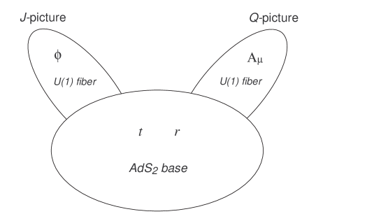
Figure 1: Twofold conformal symmetries associated with the Kerr-Newman black holes.

Therefore, in addition to the mass, every one of the other two macroscopic hairs of the KN black hole, either the angular momentum or the charge, can provide an individual holographically dual CFT₂ description. Actually, it has been discussed that for the higher dimensional rotating black holes, each angular momentum can provide an individual dual CFT₂, see for example Lu:2008jk ; Chen:2009xja . According to our results, the charge of black holes also shares the same property. Hence, we conjecture that there should be a general property for any black hole sourced by abelian gauge fields, which could be summarized as a “microscopic no hair theorem”: for each macroscopic hair parameter, in additional to the mass of a black hole in the Einstein-Maxwell theory (with dimension $D\geq 3$), there should exist an associated holographic CFT₂ description.

Appendix A Symmetry and Casimir Operator of $\mathrm{AdS}_{3}$

The two sets of symmetry generators of the AdS₃ space with radius $L$, in the Poincaré coordinates: ($w^{\pm},y$),

$$ds_{3}^{2}=\frac{L^{2}}{y^{2}}(dy^{2}+dw^{+}dw^{-}),$$ (62)

are

$$H_{1}=i\partial_{+},\quad H_{0}=i\left(w^{+}\,\partial_{+}+\frac{1}{2}y\,\partial_{y}\right),\quad H_{-1}=i\left((w^{+})^{2}\,\partial_{+}+w^{+}y\,\partial_{y}-y^{2}\,\partial_{-}\right),$$ (63)

$$\bar{H}_{1}=i\partial_{-},\quad\bar{H}_{0}=i\left(w^{-}\,\partial_{-}+\frac{1}{2}y\,\partial_{y}\right),\quad\bar{H}_{-1}=i\left((w^{-})^{2}\,\partial_{-}+w^{-}y\,\partial_{y}-y^{2}\,\partial_{+}\right),$$ (64)

assembling two copies of the $SL(2,R)$ Lie algebra

$$\left[H_{0},H_{\pm 1}\right]=\mp iH_{\pm 1},\qquad\left[H_{-1},H_{1}\right]=-2iH_{0}.$$ (65)

Thus the corresponding Casimir operator is

$$\mathcal{H}^{2}=\bar{\mathcal{H}}^{2}=-H_{0}^{2}+\frac{1}{2}\left(H_{1}H_{-1}+H_{-1}H_{1}\right)=\frac{1}{4}\left(y^{2}\,\partial_{y}^{2}-y\,\partial_{y}\right)+y^{2}\,\partial_{+}\partial_{-}.$$ (66)

Converting the Poincaré coordinates ($w^{\pm},y$) to the coordinates ($t,r,\chi$) by the following transformations

$$w^{+} = \sqrt{\frac{r-r_{+}}{r-r_{-}}}\,\exp(2\pi T_{R}\chi+2n_{R}t),$$

$$w^{-} = \sqrt{\frac{r-r_{+}}{r-r_{-}}}\,\exp(2\pi T_{L}\chi+2n_{L}t),$$

$$y = \sqrt{\frac{r_{+}-r_{-}}{r-r_{-}}}\,\exp[\pi(T_{R}+T_{L})\chi+(n_{R}+n_{L})t],$$ (67)

we can directly calculate all the $SL(2,R)$ generators in terms of black hole coordinates

$$H_{1} = i\mathrm{e}^{-(2\pi T_{R}\chi+2n_{R}t)}\left[\sqrt{\Delta}\partial_{r}\!+\!\frac{n_{L}(\delta_{-}\!+\!\delta_{+})\!+\!n_{R}(\delta_{-}\!-\!\delta_{+})}{4\pi\sqrt{\Delta}\mathcal{A}}\partial_{\chi}\!-\!\frac{T_{L}(\delta_{-}\!+\!\delta_{+})\!+\!T_{R}(\delta_{-}\!-\!\delta_{+})}{4\sqrt{\Delta}\mathcal{A}}\,\partial_{t}\right],$$

$$H_{0} = i\left[\frac{n_{L}}{2\pi\mathcal{A}}\,\partial_{\chi}-\frac{T_{L}}{2\mathcal{A}}\,\partial_{t}\right],$$

$$H_{-1} = i\mathrm{e}^{2\pi T_{R}\chi+2n_{R}t}\left[-\sqrt{\Delta}\partial_{r}\!+\!\frac{n_{L}(\delta_{-}\!+\!\delta_{+})\!+\!n_{R}(\delta_{-}\!-\!\delta_{+})}{4\pi\sqrt{\Delta}\mathcal{A}}\partial_{\chi}\!-\!\frac{T_{L}(\delta_{-}\!+\!\delta_{+})\!+\!T_{R}(\delta_{-}\!-\!\delta_{+})}{4\sqrt{\Delta}\mathcal{A}}\,\partial_{t}\right],$$

and

$$\bar{H}_{1} = i\mathrm{e}^{-(2\pi T_{L}\chi+2n_{L}t)}\left[\sqrt{\Delta}\partial_{r}\!-\!\frac{n_{R}(\delta_{-}\!+\!\delta_{+})\!+\!n_{L}(\delta_{-}\!-\!\delta_{+})}{4\pi\sqrt{\Delta}\mathcal{A}}\partial_{\chi}\!+\!\frac{T_{R}(\delta_{-}\!+\!\delta_{+})\!+\!T_{L}(\delta_{-}\!-\!\delta_{+})}{4\sqrt{\Delta}\mathcal{A}}\,\partial_{t}\right],$$

$$\bar{H}_{0} = i\left[-\frac{n_{R}}{2\pi\mathcal{A}}\,\partial_{\chi}-\frac{T_{R}}{2\mathcal{A}}\,\partial_{t}\right],$$

$$\bar{H}_{-1} = i\mathrm{e}^{2\pi T_{L}\chi+2n_{L}t}\left[-\sqrt{\Delta}\partial_{r}\!-\!\frac{n_{R}(\delta_{-}\!+\!\delta_{+})\!+\!n_{L}(\delta_{-}\!-\!\delta_{+})}{4\pi\sqrt{\Delta}\mathcal{A}}\partial_{\chi}\!+\!\frac{T_{R}(\delta_{-}\!+\!\delta_{+})\!+\!T_{L}(\delta_{-}\!-\!\delta_{+})}{4\sqrt{\Delta}\mathcal{A}}\,\partial_{t}\right],$$

where

$$\delta_{\pm}=r-r_{\pm},\qquad\mathcal{A}=T_{R}n_{L}-T_{L}n_{R}.$$ (68)

Finally the Casimir operator becomes

$$\mathcal{H}^{2}=\partial_{r}(\Delta\partial_{r})-\frac{r_{+}-r_{-}}{r-r_{+}}\left(\frac{T_{L}+T_{R}}{4\mathcal{A}}\partial_{t}-\frac{n_{L}+n_{R}}{4\pi\mathcal{A}}\partial_{\chi}\right)^{2}+\frac{r_{+}-r_{-}}{r-r_{-}}\left(\frac{T_{L}-T_{R}}{4\mathcal{A}}\partial_{t}-\frac{n_{L}-n_{R}}{4\pi\mathcal{A}}\partial_{\chi}\right)^{2}.$$ (69)

References

• (1) G. ’t Hooft, “Dimensional reduction in quantum gravity,” arXiv:gr-qc/9310026.
• (2) L. Susskind, “The world as a hologram,” J. Math. Phys.  36, 6377 (1995) [arXiv:hep-th/9409089].
• (3) J. M. Maldacena, “The large N limit of superconformal field theories and supergravity,” Adv. Theor. Math. Phys.  2, 231 (1998) [Int. J. Theor. Phys.  38, 1113 (1999)] [arXiv:hep-th/9711200].
• (4) S. S. Gubser, I. R. Klebanov and A. M. Polyakov, “Gauge theory correlators from non-critical string theory,” Phys. Lett.  B 428, 105 (1998) [arXiv:hep-th/9802109].
• (5) E. Witten, “Anti-de Sitter space and holography,” Adv. Theor. Math. Phys.  2, 253 (1998) [arXiv:hep-th/9802150].
• (6) M. Guica, T. Hartman, W. Song and A. Strominger, “The Kerr/CFT correspondence,” Phys. Rev.  D 80, 124008 (2009) [arXiv:0809.4266 [hep-th]].
• (7) O. J. C. Dias, H. S. Reall and J. E. Santos, “Kerr-CFT and gravitational perturbations,” JHEP 0908, 101 (2009) [arXiv:0906.2380 [hep-th]].
• (8) Y. Matsuo, T. Tsukioka and C. M. Yoo, “Another Realization of Kerr/CFT Correspondence,” Nucl. Phys.  B 825, 231 (2010) [arXiv:0907.0303 [hep-th]].
• (9) I. Bredberg, T. Hartman, W. Song and A. Strominger, “Black Hole Superradiance From Kerr/CFT,” JHEP 1004, 019 (2010) [arXiv:0907.3477 [hep-th]].
• (10) A. J. Amsel, D. Marolf and M. M. Roberts, “On the Stress Tensor of Kerr/CFT,” JHEP 0910, 021 (2009) [arXiv:0907.5023 [hep-th]].
• (11) T. Hartman, W. Song and A. Strominger, “Holographic Derivation of Kerr-Newman Scattering Amplitudes for General Charge and Spin,” JHEP 1003, 118 (2010) [arXiv:0908.3909 [hep-th]].
• (12) A. Castro and F. Larsen, “Near Extremal Kerr Entropy from $AdS_{2}$ Quantum Gravity,” JHEP 0912, 037 (2009) [arXiv:0908.1121 [hep-th]].
• (13) M. Cvetic and F. Larsen, “Greybody Factors and Charges in Kerr/CFT,” JHEP 0909, 088 (2009) [arXiv:0908.1136 [hep-th]].
• (14) T. Hartman, K. Murata, T. Nishioka and A. Strominger, “CFT duals for extreme black holes,” JHEP 0904, 019 (2009) [arXiv:0811.4393 [hep-th]].
• (15) M. R. Garousi and A. Ghodsi, “The RN/CFT Correspondence,” Phys. Lett.  B 687, 79 (2010) [arXiv:0902.4387 [hep-th]].
• (16) C. M. Chen, Y. M. Huang and S. J. Zou, “Holographic Duals of Near-extremal Reissner-Nordstrom Black Holes,” JHEP 1003, 123 (2010) [arXiv:1001.2833 [hep-th]].
• (17) C. M. Chen, J. R. Sun and S. J. Zou, “The RN/CFT Correspondence Revisited,” JHEP 1001, 057 (2010) [arXiv:0910.2076 [hep-th]].
• (18) K. Hotta, Y. Hyakutake, T. Kubota, T. Nishinaka and H. Tanida, “The CFT-interpolating Black Hole in Three Dimensions,” JHEP 0901, 010 (2009) [arXiv:0811.0910 [hep-th]].
• (19) H. Lu, J. Mei and C. N. Pope, “Kerr/CFT Correspondence in Diverse Dimensions,” JHEP 0904, 054 (2009) [arXiv:0811.2225 [hep-th]].
• (20) T. Azeyanagi, N. Ogawa and S. Terashima, “Holographic Duals of Kaluza-Klein Black Holes,” JHEP 0904, 061 (2009) [arXiv:0811.4177 [hep-th]].
• (21) D. D. K. Chow, M. Cvetic, H. Lu and C. N. Pope, “Extremal Black Hole/CFT Correspondence in (Gauged) Supergravities,” Phys. Rev.  D 79, 084018 (2009) [arXiv:0812.2918 [hep-th]].
• (22) T. Azeyanagi, N. Ogawa and S. Terashima, “The Kerr/CFT Correspondence and String Theory,” Phys. Rev.  D 79, 106009 (2009) [arXiv:0812.4883 [hep-th]].
• (23) Y. Nakayama, “Emerging AdS from extremally rotating NS5-branes,” Phys. Lett.  B 673, 272 (2009) [arXiv:0812.2234 [hep-th]].
• (24) H. Isono, T. S. Tai and W. Y. Wen, “Kerr/CFT correspondence and five-dimensional BMPV black holes,” Int. J. Mod. Phys.  A 24, 5659 (2009) [arXiv:0812.4440 [hep-th]].
• (25) J. J. Peng and S. Q. Wu, “Extremal Kerr black hole/CFT correspondence in the five dimensional Gódel universe,” Phys. Lett.  B 673, 216 (2009) [arXiv:0901.0311 [hep-th]].
• (26) C. M. Chen and J. E. Wang, “Holographic Duals of Black Holes in Five-dimensional Minimal Supergravity,” Class. Quant. Grav.  27, 075004 (2010) [arXiv:0901.0538 [hep-th]].
• (27) F. Loran and H. Soltanpanahi, “5D Extremal Rotating Black Holes and CFT duals,” Class. Quant. Grav.  26, 155019 (2009) [arXiv:0901.1595 [hep-th]].
• (28) A. M. Ghezelbash, “Kerr/CFT correspondence in the low energy limit of heterotic string theory,” JHEP 0908, 045 (2009) [arXiv:0901.1670 [hep-th]].
• (29) H. Lu, J. w. Mei, C. N. Pope and J. F. Vazquez-Poritz, “Extremal static AdS black hole/CFT correspondence in gauged supergravities,” Phys. Lett.  B 673, 77 (2009) [arXiv:0901.1677 [hep-th]].
• (30) A. J. Amsel, G. T. Horowitz, D. Marolf and M. M. Roberts, “No Dynamics in the Extremal Kerr Throat,” JHEP 0909, 044 (2009) [arXiv:0906.2376 [hep-th]].
• (31) G. Compere, K. Murata and T. Nishioka, “Central Charges in Extreme Black Hole/CFT Correspondence,” JHEP 0905, 077 (2009) [arXiv:0902.1001 [hep-th]].
• (32) C. Krishnan and S. Kuperstein, “A Comment on Kerr-CFT and Wald Entropy,” Phys. Lett.  B 677, 326 (2009) [arXiv:0903.2169 [hep-th]].
• (33) K. Hotta, “Holographic RG flow dual to attractor flow in extremal black holes,” Phys. Rev.  D 79, 104018 (2009) [arXiv:0902.3529 [hep-th]].
• (34) D. Astefanesei and Y. K. Srivastava, “CFT Duals for Attractor Horizons,” Nucl. Phys.  B 822, 283 (2009) [arXiv:0902.4033 [hep-th]].
• (35) W. Y. Wen, “Holographic descriptions of (near-)extremal black holes in five dimensional minimal supergravity,” arXiv:0903.4030 [hep-th].
• (36) T. Azeyanagi, G. Compere, N. Ogawa, Y. Tachikawa and S. Terashima, “Higher-Derivative Corrections to the Asymptotic Virasoro Symmetry of 4d Extremal Black Holes,” Prog. Theor. Phys.  122, 355 (2009) [arXiv:0903.4176 [hep-th]].
• (37) X. N. Wu and Y. Tian, “Extremal Isolated Horizon/CFT Correspondence,” Phys. Rev.  D 80, 024014 (2009) [arXiv:0904.1554 [hep-th]].
• (38) J. J. Peng and S. Q. Wu, “Extremal Kerr/CFT correspondence of five-dimensional rotating (charged) black holes with squashed horizons,” Nucl. Phys.  B 828, 273 (2010) [arXiv:0911.5070 [hep-th]].
• (39) B. Chen, B. Ning and Z. b. Xu, “Real-time correlators in warped AdS/CFT correspondence,” JHEP 1002, 031 (2010) [arXiv:0911.0167 [hep-th]].
• (40) B. Chen and C. S. Chu, “Real-time correlators in Kerr/CFT correspondence,” JHEP 1005, 004 (2010) [arXiv:1001.3208 [hep-th]].
• (41) M. Becker, S. Cremonini and W. Schulgin, “Extremal Three-point Correlators in Kerr/CFT,” arXiv:1004.1174 [hep-th].
• (42) V. Balasubramanian, J. de Boer, M. M. Sheikh-Jabbari and J. Simon, “What is a chiral 2d CFT? And what does it have to do with extremal black holes?,” JHEP 1002, 017 (2010) [arXiv:0906.3272 [hep-th]].
• (43) A. Castro, C. Keeler and F. Larsen, “Three Dimensional Origin of $AdS_{2}$ Quantum Gravity,” arXiv:1004.0554 [hep-th].
• (44) J. D. Brown and M. Henneaux, “Central charges in the canonical realization of asymptotic symmetries: an example from three-dimensional gravity,” Commun. Math. Phys.  104, 207 (1986).
• (45) A. Castro, A. Maloney and A. Strominger, “Hidden Conformal Symmetry of the Kerr Black Hole,” arXiv:1004.0996 [hep-th].
• (46) C. M. Chen and J. R. Sun, “Hidden Conformal Symmetry of the Reissner-Nordstrom Black Holes,” arXiv:1004.3963 [hep-th].
• (47) C. Krishnan, “Hidden Conformal Symmetries of Five-Dimensional Black Holes,” arXiv:1004.3537 [hep-th].
• (48) Y. Q. Wang and Y. X. Liu, “Hidden Conformal Symmetry of the Kerr-Newman Black Hole,” arXiv:1004.4661 [hep-th].
• (49) J. Rasmussen, “A near-NHEK/CFT correspondence,” arXiv:1004.4773 [hep-th].
• (50) B. Chen and J. Long, “Real-time Correlators and Hidden Conformal Symmetry in Kerr/CFT Correspondence,” arXiv:1004.5039 [hep-th].
• (51) R. Li, M. F. Li and J. R. Ren, “Entropy of Kaluza-Klein Black Hole from Kerr/CFT Correspondence,” arXiv:1004.5335 [hep-th].
• (52) D. Chen, P. Wang and H. Wu, “Hidden conformal symmetry of rotating charged black holes,” arXiv:1005.1404 [gr-qc].
• (53) C. Krishnan, “Black Hole Vacua and Rotation,” arXiv:1005.1629 [hep-th].
• (54) J. Rasmussen, “On the CFT duals for near-extremal black holes,” arXiv:1005.2255 [hep-th].
• (55) M. Becker, S. Cremonini and W. Schulgin, “Correlation Functions and Hidden Conformal Symmetry of Kerr Black Holes,” arXiv:1005.3571 [hep-th].
• (56) B. Chen and J. Long, “On Holographic description of the Kerr-Newman-AdS-dS black holes,” arXiv:1006.0157 [hep-th].
• (57) H. Wang, D. Chen, B. Mu and H. Wu, “Hidden conformal symmetry of the Einstein-Maxwell-Dilaton-Axion black hole,” arXiv:1006.0439 [gr-qc].
• (58) C. M. Chen, Y. M. Huang, J. R. Sun, M. F. Wu and S. J. Zou, “On Holographic Dual of the Dyonic Reissner-Nordström Black Hole,” arXiv:1006.4092 [hep-th].
• (59) D. T. Son and A. O. Starinets, “Minkowski-space correlators in AdS/CFT correspondence: Recipe and applications,” JHEP 0209, 042 (2002) [arXiv:hep-th/0205051].