Statistical distribution of quantum entanglement for a random bipartite state

Abstract

We compute analytically the statistics of the Renyi and von Neumann entropies (standard measures of entanglement), for a random pure state in a large bipartite quantum system. The full probability distribution is computed by first mapping the problem to a random matrix model and then using a Coulomb gas method. We identify three different regimes in the entropy distribution, which correspond to two phase transitions in the associated Coulomb gas. The two critical points correspond to sudden changes in the shape of the Coulomb charge density: the appearance of an integrable singularity at the origin for the first critical point, and the detachement of the rightmost charge (largest eigenvalue) from the sea of the other charges at the second critical point. Analytical results are verified by Monte Carlo numerical simulations. A short account of some of these results appeared recently in Phys. Rev. Lett. 104, 110501 (2010).

1 Introduction

Entanglement plays a crucial role in quantum information and computation as a measure of nonclassical correlations between parts of a quantum system [1]. The strength of those quantum correlations is significant in highly entangled states, which are involved and exploited in powerful communication and computational tasks that are not possible classically. Random pure states are of special interest as their average entropy is close to its possible maximum value [2, 3]. Taking a quantum state at random also corresponds to assuming minimal prior knowledge about the system [4]. Random states can thus be seen as “typical states” to which an arbitrary time-evolving quantum state may be compared. In addition, random states are useful in the context of quantum chaotic or nonintegrable systems [5, 6, 7].

There exist several measures for quantifying entanglement [8]. For a bipartite quantum system, the entropy (either the von Neumann or the Renyi entropies) is a well-known measure of entanglement. For a multipartite system, the full distribution of bipartite entanglement between two parts of the system has been proposed as a measure of multipartite entanglement [9]. The distribution of entropy in a bipartite system is thus generally useful for characterizing entanglement properties of a random pure state.

Statistical properties of observables such as the von Neumann entropy, concurrence, purity or the minimum eigenvalue for random pure states have been studied extensively [2, 3, 10, 11, 12, 13, 14, 15, 16, 17]. In particular, the average von Neumann entropy is known to be close to its maximal value (for a large system). In contrast, few studies have addressed the full distribution of the entropy: only the distribution of the purity for very small systems [13] and partial information on the Laplace transform of the purity distribution for large systems [10] have previously appeared in the literature.

Our purpose here is to compute the full distribution of the Renyi entropies for a random pure state in a large bipartite quantum system. In particular, we show that the common idea that a random pure state is maximally entangled is not quite correct: while the average entropy is indeed close to its maximal value [2, 3], the probability of an almost maximally entangled state is in fact vanishingly small. This statement requires to compute the full probability distribution of the entropy, namely its large deviation tails, which is one of the goals achieved in our paper.

The calculation of the Renyi entropies’ distribution proceeds by mapping the entanglement problem to an equivalent random matrix model, which describes the statistical properties of the reduced density matrix of a subsystem. We can then use Coulomb gas methods borrowed from random matrix theory. We identify three regimes in the distribution of the entropy, as a direct consequence of two phase transitions in the associated Coulomb gas problem. One of those transitions is akin to a Bose-Einstein condensation, with one charge of the Coulomb gas detaching from the sea of the other charges - or equivalently one eigenvalue of the reduced density matrix becoming much larger than the others.

This paper is a detailed version of a short letter that was published recently [18]. It thus contains all explicit formulas for our results and details about analytical proofs and numerical simulations as well as new results, especially for the third regime of the distribution (see below), the von Neumann entropy and the maximal eigenvalue of the density matrix.

The plan of the paper is as follows. In section 2, we describe precisely our model of bipartite quantum system for the direct product $\mathcal{H}_{A}\otimes\mathcal{H}_{B}$ of two Hilbert spaces $\mathcal{H}_{A}$ and $\mathcal{H}_{B}$. In section 3, we analyze the distribution of the eigenvalues $\lambda_{i}$ of the reduced density matrices of the two subsystems. In particular, we compute the average density of eigenvalues and explain the Coulomb gas method that we also use later for computing the distribution of the Renyi entropy $S_{q}=\frac{1}{1-q}\ln\Sigma_{q}$ where $\Sigma_{q}=\sum_{i}\lambda_{i}^{q}$. In section 4, we compute the full distribution of $\Sigma_{q}$ for a large system. We find two phase transitions in the associated Coulomb gas, and thus three regimes for the distribution of $\Sigma_{q}$. In section 5, using results from section 4, we derive the distribution of the Renyi entropy $S_{q}$ as well as the distribution of the von Neumann entropy (case $q\rightarrow 1$) and the distribution of the largest eigenvalue ($q\rightarrow\infty$). Finally in section 6, we present results obtained by Monte Carlo numerical simulations that we performed to test and verify our analytical predictions.

2 Random bipartite state

In this section, we set the problem of bipartite entanglement for a random pure state. We first describe a bipartite quantum system, introduce then measures of entanglement (the von Neumann and Renyi entropies) and give finally the precise definition of random pure states.

2.1 Entanglement in a bipartite quantum system

Let us consider a bipartite quantum system $A\otimes B$ composed of two subsystems $A$ and $B$ of respective dimensions $N$ and $M$. The system is described by the product Hilbert space $\mathcal{H}_{AB}=\mathcal{H}_{A}\otimes\mathcal{H}_{B}$ with $N=\dim\left(\mathcal{H}_{A}\right)$ and $M=\dim\left(\mathcal{H}_{B}\right)$. Here, we shall be interested in the limit where $N$ and $M$ are large and $c=\frac{N}{M}$ is fixed. We shall take $N\leq M$, i.e. $c\leq 1$, so that $A$ and $B$ play the role of the subsystem of interest and of the environment, respectively.

Let $|\psi\rangle$ be a pure state of the full system. Its density matrix $\rho=|\psi\rangle\langle\psi|$ is a positive semi-definite Hermitian matrix normalized as ${\rm Tr}\,\rho=\langle\psi|\psi\rangle=1$. The density matrix can thus be diagonalized, its eigenvalues are non-negative and their sum is unity. Subsystem $A$ is described by its reduced density matrix $\rho_{A}={\rm Tr_{B}\left[\rho\right]}=\sum_{\alpha^{B}=1}^{M}\langle\alpha^{B}|\rho|\alpha^{B}\rangle$, where $|\alpha^{B}\rangle$ is an orthonormal basis of $\mathcal{H}_{B}$. Similarly, $B$ is described by $\rho_{B}={\rm Tr_{A}\left[\rho\right]}$. It is easy to show that the reduced matrices $\rho_{A}$ and $\rho_{B}$ share the same set of non-negative eigenvalues $\{\lambda_{1},...,\lambda_{N}\}$ with $\sum_{i=1}^{N}\lambda_{i}=1$.

Any pure state can be written as $|\psi\rangle=\sum_{i=1}^{N}\sum_{\alpha=1}^{M}x_{i,\alpha}\>|i^{A}\rangle\otimes|\alpha^{B}\rangle$ where $|i^{A}\rangle\otimes|\alpha^{B}\rangle$ is a fixed orthonormal basis of $\mathcal{H}_{AB}$. The singular value decomposition of the matrix $x_{i,\alpha}$ permits to recast the previous expression in the so-called Schmidt decomposition form:

$$|\psi\rangle=\sum_{i=1}^{N}\sqrt{\lambda_{i}}|m_{i}^{A}\rangle\otimes|\mu_{i}^{B}\rangle$$ (1)

where $|m_{i}^{A}\rangle$ and $|\mu_{i}^{B}\rangle$ represent the eigenvectors of $\rho_{A}$ and $\rho_{B}$, respectively, associated with the same eigenvalue $\lambda_{i}$.

The representation (1), namely the Schmidt number $n_{S}$ of strictly positive eigenvalues, is very useful for characterizing the entanglement between subsystems $A$ and $B$. For example, let us consider two limiting cases:

(i) If only one of the eigenvalues, say $\lambda_{i}$, is non zero then $\lambda_{i}=1$, $n_{S}=1$ and the state of the full system $|\psi\rangle=|m_{i}^{A}\rangle\otimes|\mu_{i}^{B}\rangle$ is a product state, which is said to be separable. The system is unentangled.

(ii) If all the eigenvalues are equal ($\lambda_{j}=1/N$ for all $j$), $n_{S}=N$ and $|\psi\rangle$ is a superposition of all product states. The system is maximally entangled.

A standard measure of entanglement between two subsystems $A$ and $B$ is the von Neumann entropy of either subsystem: $S_{\rm VN}=-{\rm Tr}\left[\rho_{A}\ln\rho_{A}\right]=-\sum_{i=1}^{N}\lambda_{i}\ln\lambda_{i}$, which reaches its minimum $0$ when the system is unentangled (situation (i) above) and its maximum $\ln N$ when the system is maximally entangled (situation (ii)). Another useful measure of entanglement is the Renyi entropy of order $q$ (for $q>0$):

$$S_{q}=\frac{1}{1-q}\,\ln\left[\sum_{i=1}^{N}\lambda_{i}^{q}\right]\,,$$ (2)

which also reaches its minimal value $0$ in situation (i) and its maximal value $\ln N$ in situation (ii). As one varies the parameter $q$, the Renyi entropy interpolates between the von Neumann entropy ($q\rightarrow 1^{+}$) and $-\ln\lambda_{\rm max}$ ($q\rightarrow\infty$) where $\lambda_{\rm max}$ is the largest eigenvalue of the reduced density matrices.

2.2 Random pure states

A pure state is called random when it is sampled according to the uniform Haar measure, which is unitarily invariant. Specifically, a random pure state is defined as $|\psi\rangle=\sum_{i=1}^{N}\sum_{\alpha=1}^{M}x_{i,\alpha}\>|i^{A}\rangle\otimes|\alpha^{B}\rangle$, where $|i^{A}\rangle\otimes|\alpha^{B}\rangle$ is a fixed orthonormal basis of $\mathcal{H}_{AB}$ and where the variables $\left\{x_{i,\alpha}\right\}$ are uniformly distributed among the sets of $\left\{x_{i,\alpha}\right\}$ satisfying the constraint $\sum_{i,\alpha}\left|x_{i,\alpha}\right|^{2}=1$ (normalization of $|\psi\rangle$). Equivalently, the probability density function (pdf) of the $N\times M$ matrix $X$ with entries $x_{i,\alpha}$ can be written

$$P(X)\propto\delta\left({\rm Tr}(XX^{\dagger})-1\right)\propto e^{-\frac{\beta}{2}{\rm Tr}(XX^{\dagger})}\;\delta({\rm Tr}(XX^{\dagger})-1)\,,$$ (3)

with the second equality showing that the pdf can also be seen as a Gaussian supplemented by the unit-trace constraint.

In the basis $|i^{A}\rangle$ of $\mathcal{H}_{A}$, the reduced density matrix of subsystem $\mathcal{A}$ is simply given by $\rho_{A}=XX^{\dagger}$. In general, when $X$ is a $N\times M$ Gaussian random matrix, i.e. $P(X)\propto e^{-\frac{\beta}{2}{\rm Tr}(XX^{\dagger})}$ (iid Gaussian entries $x_{i,\alpha}$ that are real for a Dyson index $\beta=1$, complex for $\beta=2$), the $N\times N$ matrix $XX^{\dagger}$ is a Wishart matrix whose distribution of eigenvalues is [19]:

$$P_{Wishart}(\lambda_{1},...,\lambda_{N})\propto e^{-\frac{\beta}{2}\sum_{i}\lambda_{i}}\>\prod_{i=1}^{N}\lambda_{i}^{\frac{\beta}{2}(M-N+1)-1}\>\prod_{i<j}|\lambda_{i}-\lambda_{j}|^{\beta}\,.$$ (4)

The Vandermonde determinant $\prod_{i<j}|\lambda_{i}-\lambda_{j}|^{\beta}$ makes that the eigenvalues are strongly correlated and they physically tend to repel each other.

The major difference between the matrix $\rho_{A}=XX^{\dagger}$ in the quantum problem and a standard Wishart matrix stems from the unit trace constraint ${\rm Tr}\left[\rho_{A}\right]=1$. The constraint is to be included in the distribution of the eigenvalues of $\rho_{A}$, which is given [3, 11] by:

$$P(\lambda_{1},...,\lambda_{N})=B_{M,N}\;\delta\big{(}\sum_{i}\lambda_{i}-1\big{)}\;\prod_{i=1}^{N}\lambda_{i}^{\frac{\beta}{2}(M-N+1)-1}\>\prod_{i<j}|\lambda_{i}-\lambda_{j}|^{\beta}\,,$$ (5)

with $\beta=2$ (the $x_{i,\alpha}$ are complex) and the normalization constant $B_{M,N}$ computed using Selberg’s integrals [11]:

$$B_{M,N}=\frac{\Gamma(MN\beta/2)\,\Gamma(1+\beta/2)^{N}}{\prod_{j=0}^{N-1}\Gamma((M-j)\beta/2)\,\Gamma(1+(N-j)\beta/2)}\,.$$ (6)

The presence of a fixed trace constraint (as in Eq. (5)) is known to have important consequences on the spectral properties of a matrix [20, 21]. We will see that in the present context also, the fixed trace constraint does play an important and crucial role. In particular, this constraint is directly responsible for a Bose-Einstein type condensation transition that will be discussed in the context of the probability distribution of the entanglement entropy.

Since the eigenvalues $\lambda_{i}$ of $\rho_{A}$ are random variables for a random pure state, any observable is a random variable as well. Statistical properties of observables, namely of various measures of entanglement such as the von Neumann entropy [3, 22], $G$-concurrence [12], purity [10, 13] or minimum eigenvalue [14, 15, 16, 17], have been studied extensively. In particular, Page [3] computed the average von Neumann entropy in the limit $M\geq N\gg 1$: $\langle S_{VN}\rangle\approx\ln N-\frac{N}{2M}$. He also conjectured its value for finite $N$ and $M$ (which was proved later [22]). In contrast, there have been few studies on the full distribution of the entropy, except for the purity $\Sigma_{2}=\sum_{i}\lambda_{i}^{2}$ whose distribution is known exactly for small $N$ ($2,3$ and $4$) [13]. For large $N$, the Laplace transform of the purity distribution (generating function of the cumulants) was studied recently [10] for positive values of the Laplace variable. However, when inverted, the previous quantity provides only partial information about the purity distribution.

Here, we compute analytically the full distribution of the Renyi entropy $S_{q}$ (defined in Eq. (2)) or equivalently of $\Sigma_{q}=\sum_{i=1}^{N}\lambda_{i}^{q}=\exp{\left[(1-q)S_{q}\right]}$, for large $N$. As for the von Neumann entropy, the average value of the Renyi entropies is close to their maximal value $\ln N$ (maximal entanglement) : $\langle S_{q}\rangle\approx\ln N-\bar{z}(q)$, where $\bar{z}(q)>0$ (for $q>0$) is independent of $N$ for large $N$. For example, for $M\approx N$ and $q=2$, we have $\bar{z}(q=2)=\ln 2$. However, we show below that the probability that $S_{q}$ approaches its maximal value $\ln N$ is again very small.

3 Distribution of the eigenvalues of $\rho_{A}$

The eigenvalues of the reduced density matrix $\rho_{A}$ are distributed according to the law in Eq. (5). Given this joint distribution, the first natural object to study is the average spectral density $\rho_{N,M}(\lambda)=\frac{1}{N}\sum_{i=1}^{N}\left\langle\delta\left(\lambda-\lambda_{i}\right)\right\rangle$. This average density $\rho_{N,M}\left(\lambda\right)d\lambda$ also gives the probability to find an eigenvalue between $\lambda$ and $\lambda+d\lambda$ (the one-point marginal of the joint distribution). For finite $(N,M)$, this average density was computed first for $\beta=2$ [23, 24] and very recently for $\beta=1$ [25]. However, these formulae involve rather complicated special functions and taking the asymptotic large $N$, large $M$ limit is nontrivial. Here we will take a complementary route which is well suited to derive exactly the asymptotic limit. We will take the limit $N\to\infty$, $M\to\infty$ but keeping their ratio $0\leq c=N/M\leq 1$ fixed. For the spectral density, we will henceforth use a shorthand notation $\rho_{N}(\lambda)=\rho_{N,N/c}(\lambda)$. We will show that for large $N$ the limiting form of $\rho_{N}(\lambda)$ can be obtained easily via using a Coulomb gas approach.

Due to the unit trace constraint $\sum_{i=1}^{N}\lambda_{i}=1$, the typical amplitude of the eigenvalues is $\lambda_{typ}\sim\frac{1}{N}$ for large $N$. Since $\lambda_{typ}\sim\frac{1}{N}$ (and $\rho_{N}$ is normalized to unity), we expect (as will be proved below) that the average density for large $N$ has a scaling form:

$$\rho_{N}\left(\lambda\right)\approx N\;\rho^{*}\left(\lambda N\right)\,.$$ (7)

Using the Coulomb gas method explained in subsection 3.1, we find an exact expression for the rescaled density $\rho^{*}(x)$:

$$\rho^{*}(x)=\frac{1}{2\pi cx}\sqrt{x-L_{1}}\>\sqrt{L_{2}-x}\,,$$ (8)

where the right and left edges read $L_{2}=c\left(\sqrt{\frac{1}{c}}+1\right)^{2}$, $L_{1}=c\left(\sqrt{\frac{1}{c}}-1\right)^{2}$ and we recall that $c=N/M\leq 1$.

For $c=1$ ($N\approx M$), $L_{1}=0$, $L_{2}=4$ and the rescaled density reduces to:

$$\rho^{*}(x)=\frac{1}{2\pi}\sqrt{\frac{4-x}{x}}\,.$$ (9)

In Fig. 1, plots of the rescaled density $\rho^{*}(x)$ and comparisons to the shape of the rescaled density for a standard Wishart matrix are shown for $c=1$ and $c=1/3$.

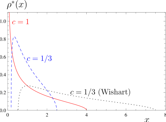
Figure 1: The rescaled average density $\rho^{*}(x)$ of the eigenvalues for the density matrix of a quantum subsystem. The rescaled density is defined by $\rho_{N}\left(\lambda\right)\approx N\;\rho^{*}\left(\lambda N\right)$ for large $N$ (see Eq. (8)) and is plotted for $c=\frac{N}{M}=1$ (red solid line) and $c=1/3$ (blue dashed line). The density is compared with the rescaled average density of Wishart eigenvalues (random matrix theory) : $\rho^{*}_{W}(x)$ defined by $\rho_{N}^{W}\left(\lambda\right)\approx\frac{1}{N}\>\;\rho^{*}_{W}\left(\frac{\lambda}{N}\right)$ (see Eq. (17)) plotted for $c=\frac{N}{M}=1$ (red solid line) and $c=1/3$ (black dotted line). The different dependencies on $c$ for $\rho^{*}(x)$ and $\rho^{*}_{W}(x)$ make that, even after their different rescaling in $N$, the two distributions are equal only for $c=1$.

3.1 Computation of the rescaled density: Coulomb gas method

The goal of this section is to prove Eqs. (7) and (8) for the average density of states. The joint distribution of the eigenvalues in Eq. (5) can be interepreted as a Boltzmann weight at inverse temperature $\beta$

$$P(\lambda_{1},...,\lambda_{N})\propto\exp\left\{-\beta E\left[\left\{\lambda_{i}\right\}\right]\right\}\,,$$ (10)

where the effective energy is given by

$$E\left[\left\{\lambda_{i}\right\}\right]=-\gamma\sum_{i=1}^{N}\ln\lambda_{i}-\sum_{i<j}\ln\left|\lambda_{i}-\lambda_{j}\right|\;\;{\rm with}\;\;\sum_{i}\lambda_{i}=1\,.$$ (11)

Here, $\gamma=\frac{M-N+1}{2}-\frac{1}{\beta}\approx N\frac{(1-c)}{2c}$ for large $N$. The logarithmic binary interactions correspond to the Coulomb repulsion in $2$ dimensions. The eigenvalues can thus be seen as charges of a $2D$ Coulomb gas, repelling each other electrostatically. The charges are confined in the segment $1\geq\lambda_{i}\geq 0$ for all $i$ and they are also subject to an external logarithmic potential (with amplitude $\gamma$).

The mapping from random matrix eigenvalues to a Coulomb gas problem is well-known in random matrix theory and has been recently used in a variety of contexts that include the distribution of the extreme eigenvalues of Gaussian and Wishart matrices [26, 27, 28, 29], purity partition function in bipartite systems [10], nonintersecting Brownian interfaces [30], quantum transport in chaotic cavities [31], information and communication systems [32], and the index distribution for Gaussian random fields [33, 34] and Gaussian matrices [35]. Here, we use similar methods yet the problem is quite different due to the constraint $\sum_{i}\lambda_{i}=1$. First, the scaling with $N$ (for large $N$) differs from standard Wishart matrices. Indeed, $\lambda_{typ}\sim 1/N$ in our problem of entanglement whereas $\lambda_{typ}^{W}\sim N$ for a Wishart matrix. However, the effect of the constraint $\sum_{i}\lambda_{i}=1$ is not just the rescaling of standard Wishart results by a factor of $1/N^{2}$ as it may seem. It turns out that the constraint has more serious consequences and leads to fundamentally different and new behavior (including a condensation transition which is absent in Wishart matrices) that we will demonstrate.

Configurations of the eigenvalues are characterized by the density $\rho(\lambda,N)=N^{-1}\sum_{i=1}^{N}\delta\left(\lambda-\lambda_{i}\right)$. For large $N$, the eigenvalues are expected to be close to each other and their typical amplitude is $\lambda_{typ}\sim\frac{1}{N}$. We introduce then a rescaled variable $x\sim O(1)$ as $x=\lambda N$. The corresponding density is $\rho(x)=N^{-1}\sum_{i=1}^{N}\delta\left(x-\lambda_{i}N\right)$, so that $\rho(\lambda,N)=N\,\rho(\lambda N)=N\,\rho(x)$.

The effective energy in Eq. (11) becomes in the continuous limit (large $N$) a functional of the density $\rho$. To the leading order in $N$, the effective energy reads $E\left[\left\{\lambda_{i}\right\}\right]=N^{2}\,E\left[\rho\right]+O(N)$, where

$$E\left[\rho\right] = -\left(\frac{1-c}{2c}\right)\int_{0}^{\infty}dx\>\rho(x)\ln x-\frac{1}{2}\int_{0}^{\infty}\int_{0}^{\infty}dxdx^{\prime}\>\rho(x)\rho(x^{\prime})\,\ln\left|x-x^{\prime}\right|$$ (12)

$$+\,\mu_{0}\left(\int_{0}^{\infty}dx\>\rho(x)-1\right)+\,\mu_{1}\left(\int_{0}^{\infty}dx\>x\,\rho(x)-1\right)\,.$$

The Lagrange multipliers $\mu_{0}$ and $\mu_{1}$ enforce respectively the constraints $\int\rho=1$ (normalization) and $\int dx\,x\,\rho(x)=1$ (unit trace).

The joint distribution of the eigenvalues is given by the Boltzmann weight $P(\lambda_{1},...,\lambda_{N})\propto\exp\left\{-\beta N^{2}E[\rho]+O(N)\right\}$ for large $N$. This distribution is highly peaked around its most probable value $\rho^{*}$ which is thus also the mean value of $\rho$: $\rho^{*}(x)=N^{-1}\sum_{i=1}^{N}\langle\delta\left(x-\lambda_{i}N\right)\rangle$. Hence, the average density of states is the continuous density $\rho^{*}$ that minimizes the effective energy: $\frac{\delta E}{\delta\rho}\Big{|}_{\rho=\rho^{*}}=0$. From Eq. (12) we get the saddle point equation for $\rho^{*}$:

$$\int_{0}^{\infty}dx^{\prime}\>\rho^{*}(x^{\prime})\,\ln\left|x-x^{\prime}\right|=\,\mu_{0}+\,\mu_{1}\>x-\left(\frac{1-c}{2c}\right)\,\ln x\,.$$ (13)

Differentiating with respect to $x$ leads to the integral equation:

$$\mathcal{P}\int_{0}^{\infty}dx^{\prime}\>\frac{\rho^{*}(x^{\prime})}{x-x^{\prime}}=\mu_{1}-\left(\frac{1-c}{2c}\right)\frac{1}{x}\,,$$ (14)

where $\mathcal{P}$ denotes the principal value. This singular integral equation can be solved by using a theorem due to Tricomi [36] that states that if the solution $\rho^{*}$ has a finite support $[L_{1},L_{2}]$, then the finite Hilbert transform defined by the equation $F(x)=\mathcal{P}\int_{L_{1}}^{L_{2}}dx^{\prime}\>\frac{\rho^{*}(x^{\prime})}{x-x^{\prime}}$ can be inverted as

$$\rho^{*}(x)=\frac{1}{\pi\sqrt{x-L_{1}}\sqrt{L_{2}-x}}\left[C-\mathcal{P}\int_{L_{1}}^{L_{2}}\frac{dx^{\prime}}{\pi}\frac{\sqrt{x^{\prime}-L_{1}}\sqrt{L_{2}-x^{\prime}}}{x-x^{\prime}}\,F(x^{\prime})\right]\,,$$ (15)

where the constant $C$ fixes the integral of $\rho^{*}$ via $\int_{L_{1}}^{L_{2}}dx\,\rho^{*}(x)=C$.

In Eq. (14), $F(x)=\mu_{1}-\left(\frac{1-c}{2c}\right)\frac{1}{x}$. Physically, the average density is expected to be smooth and thus to vanish at $L_{1}$ and $L_{2}$ (bounds of its support): $\rho^{*}(L_{1})=0=\rho^{*}(L_{2})$. These two constraints fix the value of $L_{1}$ and $L_{2}$. The other two constraints $\int\rho^{*}=1$ and $\int x\rho^{*}=1$ give the value of the constant $C$ in Eq. (15) and the Lagrange multiplier $\mu_{1}$ in Eq. (14). Finally, inserting the expression of $\rho^{*}$ in Eq. (13) for a special value of $x$ (say $x=L_{2}$) gives $\mu_{0}$. Imposing all these constraints, we finally get:

$$\rho^{*}(x)=\frac{1}{2\pi c\,x}\sqrt{x-L_{1}}\,\sqrt{L_{2}-x}\,,$$ (16)

with $L_{1,2}=c\left(1\mp\sqrt{\frac{1}{c}}\right)^{2}$ (where $c=N/M$). We also find $C=\int\rho^{*}=1$, $\mu_{1}=1/\left(2c\right)$ and $\mu_{0}=-\left(\frac{1+c}{2c}\right)+2\left(1-\frac{1}{c}\right)\ln\left[1+\sqrt{c}\right]+\frac{\ln c}{2}$. Finally, the average density in the original variable $\lambda$ is given by $\rho_{N}\left(\lambda\right)=N\>\rho^{*}\left(\lambda N\right)$, where $\rho^{*}(x)$ is given in Eq. (16).

3.2 Comparison with Wishart eigenvalues

For Wishart matrices, it is known that the average density of the eigenvalues is given, for large $N$ and fixed $c=N/M$, by the Marc̆enko-Pastur law [37]:

$$\rho_{N}^{W}\left(\lambda\right)\approx\frac{1}{N}\>\;\rho^{*}_{W}\left(\frac{\lambda}{N}\right)\;\;{\rm with}\;\;\rho^{*}_{W}(x)=\frac{1}{2\pi x}\sqrt{x-L_{1}^{W}}\>\sqrt{L_{2}^{W}-x}\,,$$ (17)

with the right and left edges given by $L_{2}^{W}=\left(1+\sqrt{\frac{1}{c}}\right)^{2}$ and $L_{1}^{W}=\left(1-\sqrt{\frac{1}{c}}\right)^{2}$.

As expected, the scaling with $N$ is different: $\lambda_{typ}^{W}\sim N$ for a Wishart eigenvalue, whereas the unit trace constraint makes that $\lambda_{typ}\sim 1/N$ for an eigenvalue of the quantum density matrix $\rho_{A}$.

For $c=1$, the two edges $L_{1}^{W}=0$, $L_{2}^{W}=4$ and $\rho^{*}_{W}(x)=\rho^{*}(x)$. However, for a general $c<1$ the rescaled densities are not quite the same (even though they have the same shape): $\rho^{*}_{W}(x)=c\>\rho^{*}(xc)$. Figure 1 shows a comparative plot of $\rho^{*}_{W}(x)$ and $\rho^{*}(x)$ for $c=1$ and $c=1/3$.

4 Distribution of $\Sigma_{q}=\sum_{i}\lambda_{i}^{q}$ for $q>1$ and $c=1$

This section is somewhat long as it contains the bulk of the details of our calculations. Hence it is useful to start with a summary of the main results obtained in subsections 4.1-4.3 as well as the main picture that emerges out of these calculations. Readers not interested in details can skip the subsections 4.1-4.3 and get the main picture just from this summary.

In this section, we compute the full distribution of $\Sigma_{q}=\sum_{i}\lambda_{i}^{q}$, and thus of the Renyi entropy $S_{q}=\ln\left(\Sigma_{q}\right)/(1-q)$ for large $N$. We take for simplicity $M\approx N$, i.e. $c=1$, but our method can be easily extended to $c<1$ as well. For simplicity, we will also restrict ourselves to the case $q\geq 1$. However, our method is also easily extendable to the case $0<q<1$. Since $\sum_{i}\lambda_{i}=1$ and $x\rightarrow x^{q}$ is convex for $q>1$, we have $N^{1-q}\leq\Sigma_{q}\leq 1$ (or equivalently $\ln N\geq S_{q}\geq 0$). The lower bound $\Sigma_{q}=N^{1-q}$ corresponds to the maximally entangled case (situation (ii) in subsection 2.1), when $\lambda_{j}=1/N$ for all $j$: the entropy is $S_{q}=\ln N$. The upper bound $\Sigma_{q}=1$ corresponds to the unentangled case (situation (i) in subsection 2.1) when only one of the $\lambda_{i}$ is non zero (and thus equal to one): the entropy is zero.

The scaling $\lambda_{typ}\sim 1/N$ implies that $\Sigma_{q}\sim N^{1-q}$ for large $N$. Let $s\equiv\Sigma_{q}\>N^{q-1}$ be the rescaled variable $s\sim O(1)$. In figure 2, a typical plot of the probability density function (pdf) $P\left(\Sigma_{q}=N^{1-q}\,s\right)$ is shown: the distribution has a Gaussian peak (centered on the mean value $s=\bar{s}(q)$) flanked on both sides by non-Gaussian tails. We show below that there are two critical values $s=s_{1}(q)$ and $s=s_{2}(q)$ separating three regimes I ($1\leq s<s_{1}(q)$), II ($s_{1}(q)<s<s_{2}(q)$) and III ($s_{2}(q)<s$).

At the first critical point $s_{1}(q)$, the distribution has a weak singularity (discontinuity of the third derivative). At the second critical point $s_{2}(q)$, a Bose-Einstein type condensation transition occurs and the distribution changes shape abruptly (first derivative is discontinuous in the limit $N\rightarrow+\infty$). These changes are a direct consequence of two phase transitions in the associated Coulomb gas problem, more precisely in the shape of the optimal charge density. The schematic plot of the distribution of $\Sigma_{q}$ (for large $N$) in Fig. 2 clearly shows the three regimes I, II and III and the discontinuity of the derivative at $s=s_{2}$ (transition between II and III).

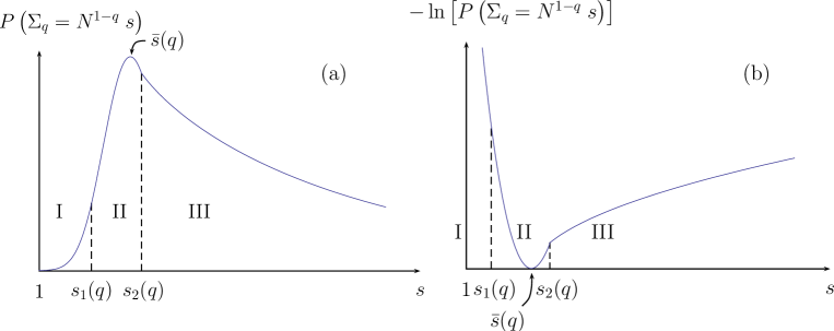
Figure 2: Schematic distribution of $\Sigma_{q}=\sum_{i}\lambda_{i}^{q}=N^{1-q}\,s$ as a function of $s$ for (very) large $N$. Panel (a) shows the shape of the pdf of $\Sigma_{q}$, while (b) shows the shape of the rate function $-\ln P(\Sigma_{q}=N^{1-q}s)$. Two critical points $s_{1}(q)$ and $s_{2}(q)$ separate three regimes I, II and III, characterized by the different optimal densities shown in figure 3. The maximally entangled state $s=1$ is at the extreme-left of the distribution, well spaced from the mean value $\bar{s}(q)$.

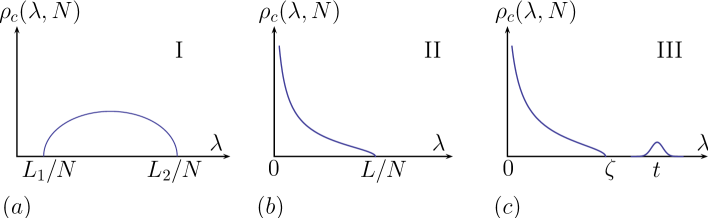
Figure 3: Scheme of the optimal saddle point density $\rho_{c}$ of the eigenvalues (or, equivalently, of the Coulomb gas of charges) for (a) $1\leq s<s_{1}(q)$ (regime I), (b) $s_{1}(q)<s<s_{2}(q)$ (regime II) and (c) $s>s_{2}(q)$ (regime III). In regime III, the maximal eigenvalue $\lambda_{\rm max}=t$ becomes much larger than the other eigenvalues, as shown by the isolated bump in (c).

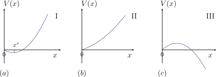
Figure 4: Scheme of the effective potential $V(x)$ seen by the charges of the Coulomb gas (eigenvalues) for (a) $1\leq s<s_{1}(q)$ (regime I), (b) $s_{1}(q)<s<s_{2}(q)$ (regime II) and (c) $s>s_{2}(q)$ (regime III). In regimes I and II, the charges are confined close to the minimum of the effective potential. In regime III, the potential is not anymore bounded from below. Therefore, one charge detaches from the sea of the other charges : the maximal eigenvalue becomes much larger than the other.

More precisely, the probability density function of $\Sigma_{q}$ for large $N$ and $q>1$ displays three different regimes:

$$P\left(\Sigma_{q}=N^{1-q}\,s\right)\approx\left\{\begin{array}[]{ll}\exp\left\{-\beta N^{2}\Phi_{I}(s)\right\}&{\rm for}\;\;1\leq s<s_{1}(q)\,;\\ &\\ \exp\left\{-\beta N^{2}\Phi_{II}(s)\right\}&{\rm for}\;\;s_{1}(q)<s<s_{2}(q)\,;\\ &\\ \exp\left\{-\beta N^{1+\frac{1}{q}}\;\Psi_{III}(s)\right\}&{\rm for}\;\;s>s_{2}(q)\,.\end{array}\right.$$ (18)

The exact mathematical meaning of the “$\approx$” sign is a logarithmic equivalence : $-\frac{\ln P\left(\Sigma_{q}=N^{1-q}\,s\right)}{\beta N^{2}}\longrightarrow\Phi_{I}(s)$ as $N\rightarrow\infty$ with fixed $s\in[1,s_{1}(q)[$ (resp. $\Phi_{II}$ for fixed $s\in]s_{1}(q),s_{2}(q)[$) and $-\frac{\ln P\left(\Sigma_{q}=N^{1-q}\,s\right)}{\beta N^{1+1/q}}\longrightarrow\Psi_{III}(s)$ as $N\rightarrow\infty$ with fixed $s>s_{2}(q)$. The rate functions $\Phi_{I}$, $\Phi_{II}$ and $\Psi_{III}$ (as well as $s_{1}$ and $s_{2}$) are independent of $N$ - but they depend on the parameter $q$. Explicit expressions of the functions $\Phi_{I}$ and $\Phi_{II}$ are given in Eqs. (38) and (42) for $q=2$, and in Eq. (47) for a general $q>1$; an explicit expression of $\Psi_{III}$ is given in Eq. (50) for a general $q>1$ (and in Eq. (51) for $q=2$). As shown in figures 5 and 6 (resp. for $N=50$ and $N=1000$), we also did some Monte Carlo simulations (as explained in section 6) and found that our analytical predictions agree very well with the numerical data.

Regime II includes the mean value $\langle\Sigma_{q}\rangle\approx N^{1-q}\bar{s}(q)$, i.e. $s_{1}(q)<\bar{s}(q)\leq s_{2}(q)$ for every $q$. The mean value is explicitely given by:

$$\langle\Sigma_{q}\rangle\approx N^{1-q}\bar{s}(q)\;\;\;{\rm with}\;\;\;\bar{s}(q)=\frac{\Gamma(q+1/2)}{\sqrt{\pi}\Gamma(q+2)}\,4^{q}\,.$$ (19)

For large $N$, the distribution of $\Sigma_{q}$ given in Eq. (18) is highly peaked around its average (because of the factor $N^{2}$ in regime II): the average value of $\Sigma_{q}$ coincides then with the most probable value, i.e. $\bar{s}(q)$ is the minimum of $\Phi_{II}(s)$. The quadratic behaviour of $\Phi_{II}(s)$ around this minimum gives the Gaussian behaviour of the distribution of $\Sigma_{q}$ around its average (and thus gives the variance of $\Sigma_{q}$). We get:

$$P\left(\Sigma_{q}=N^{1-q}s\right)\approx\exp\left\{-\beta N^{2}\frac{(s-\bar{s}(q))^{2}}{2\sigma_{q}^{2}}\right\}\;\;\textrm{for $s$ close to $\bar{s}(q)$}\,.$$ (20)

Therefore, the variance of $\Sigma_{q}$ is given by:

$${\rm Var}\,\Sigma_{q}=\langle\Sigma_{q}^{2}\rangle-\langle\Sigma_{q}\rangle^{2}\approx\frac{\sigma_{q}^{2}}{\beta N^{2q}}\;\;{\rm with}\;\;\sigma_{q}^{2}=\frac{4^{2q}}{2\pi}q(q-1)^{2}\frac{\Gamma(q+1/2)^{2}}{\Gamma(q+2)^{2}}\,.$$ (21)

The distribution has a Gaussian peak flanked by non-Gaussian tails described by the rate functions $\Phi_{I}$ (left tail) and $\Psi_{III}$ (right tail). Conversely, the rate function $\Phi_{II}$ describes the middle part of the distribution, which includes the Gaussian behaviour in the neighbourhood of the average.

In the limit $N\rightarrow\infty$, $s_{1}(q)$ and $s_{2}(q)$ do not depend on $N$ and the second critical value $s_{2}(q)$ is actually equal to the mean value $\bar{s}(q)$ of $s$:

$$s_{1}(q)=\frac{\Gamma(q+3/2)}{\sqrt{\pi}\Gamma(q+2)}\,\left(\frac{4(q+1)}{3q}\right)^{q}\;\;{\rm and}\;\;s_{2}(q)=\bar{s}(q)=\frac{\Gamma(q+1/2)}{\sqrt{\pi}\Gamma(q+2)}\,4^{q}\,.$$ (22)

However, for a large but finite $N$, $s_{2}(q,N)$ actually depends on $N$ and is given in Eq. (23) below.

The convergence in $N$ for the regimes I and II is very fast : the agreement between numerical simulations and analytical predictions in the limit $N\rightarrow\infty$ is very good already for $N\simeq 50$. However, the second transition, between regime II and III, is affected by finite-size effects, that remain important even for $N\simeq O(10^{3})$. Their main effect is a shift in the value of the critical point $s_{2}$. The transition actually occurs at a value $s_{2}(q,N)$ that depends on $N$, is a bit larger than $\bar{s}(q)$ and tends slowly to $\bar{s}(q)$ as $N\rightarrow\infty$. More precisely, the second transition occurs at $s=s_{2}(q,N)$ with

$$s_{2}(q,N)\approx\bar{s}(q)+\frac{\left[\sqrt{q/2}\,(q-1)\,\bar{s}(q)\right]^{2q/(2q-1)}}{N^{(q-1)/(2q-1)}}\;\;\;\;\textrm{for large but finite $N$}\,.$$ (23)

For example, for $q=2$, we have $\bar{s}(q=2)=2$ and $s_{2}(q=2,N)\approx 2+\frac{2^{4/3}}{N^{1/3}}-\frac{2^{5/3}\ln N}{3N^{2/3}}$ for large but finite $N$.

The extreme left of the distribution corresponds to maximally entangled states: $s\rightarrow 1^{+}$ means that $\sum_{i}\lambda_{i}^{q}=\Sigma_{q}\rightarrow N^{1-q}$, that is the case where all the eigenvalues are equal and the state is maximally entangled (situation (ii)). As $s\rightarrow 1$, $\Phi_{I}(s)$ tends to $+\infty$, thus the pdf $P(\Sigma_{q}=N^{1-q}s)$ tends rapidly towards zero. For example, for $q=2$, we have $P(\Sigma_{q}=N^{1-q}s)\approx(s-1)^{\beta N^{2}/4}$ as $s\rightarrow 1^{+}$. This implies that the probability of a maximally entangled configuration is very small (for large $N$).

Similarly, the extreme right $s\rightarrow+\infty$ of the distribution corresponds to weakly entangled states. An unentangled state has indeed only one non-zero eigenvalue, $\lambda_{i}$, thus $S=\Sigma_{q}=1$ (situation (i)). We can actually compute the expression of the pdf for the scaling $\Sigma_{q}=S$ with $S\approx O(1)$ ($S\gg s/N$) and $0<S<1$. For $q=2$, we get: $P\left(\Sigma_{2}=S\right)\approx\left(1-\sqrt{S}\right)^{\beta N^{2}/2}$ for $N\rightarrow\infty$ with $S\approx O(1)$. For $S\rightarrow 1^{-}$, the pdf of $\Sigma_{q}$ is again tending very rapidly towards zero: unentangled states are highly unlikely.

The three regimes in the distribution of $\Sigma_{q}$ are actually a direct consequence of two phase transitions in the associated Coulomb gas problem, as we show in this section. We compute the probability density function $P(\Sigma_{q}=N^{1-q}\,s)$. The charges of the associated Coulomb gas see a different effective potential $V(x)$ depending on the value of $s$, as shown by Fig. 4:

$\bullet$ In regime I ($1\leq s\leq s_{1}$), the potential $V(x)$ has a minimum at a positive $x$ and the charges accumulate near this minimum: the optimal density $\rho_{c}(\lambda,N)$ describing the charges has a finite support over $[L_{1}/N,L_{2}/N]$ and vanishes at $L_{1}/N$ and $L_{2}/N$ (see Fig. 3(a) and 4(a)).

$\bullet$ In regime II ($s_{1}<s\leq s_{2}$), the potential is minimum at $x=0$, the charges accumulate close to the origin: the optimal density $\rho_{c}(\lambda,N)$ describing the charges has a finite support over $]0,L/N]$, vanishes at $L/N$ but diverges as $1/\sqrt{\lambda}$ at the origin (see Fig. 3(b) and 4(b)).

$\bullet$ As $s$ exceeds $s_{2}$, the potential becomes unbounded from below; the rightmost charge (maximal eigenvalue) suddenly jumps far from the other eigenvalues: the charges are described in regime III by a density with finite support $]0,\zeta]$ and a single charge (maximal eigenvalue) well separated from the other charges: $t\gg\zeta$ (see Fig. 3(c) and 4(c)).

4.1 Computation of the pdf of $\Sigma_{q}$: associated Coulomb gas

In this subsection, we explain how we compute the pdf (probability density function) of $\Sigma_{q}$ using a Coulomb gas method. The pdf of $\Sigma_{q}$ is by definition:

$$P(\Sigma_{q},N)=\int P(\lambda_{1},...,\lambda_{N})\>\>\delta\left(\sum_{i}\lambda_{i}^{q}-\Sigma_{q}\right)\left(\prod_{i}d\lambda_{i}\right)\,.$$ (24)

The joint pdf of the eigenvalues $P(\lambda_{1},...,\lambda_{N})$ is given in Eq. (5) and can be seen as a Boltzmann weight at inverse temperature $\beta$, as in Eq. (10):

$$P(\lambda_{1},...,\lambda_{N})\propto\exp\left\{-\beta E\left[\left\{\lambda_{i}\right\}\right]\right\}\,,$$ (25)

where the energy $E\left[\left\{\lambda_{i}\right\}\right]=-\gamma\sum_{i=1}^{N}\ln\lambda_{i}-\sum_{i<j}\ln\left|\lambda_{i}-\lambda_{j}\right|$ (with $\sum_{i}\lambda_{i}=1$) is the effective energy of a 2D Coulomb gas of charges. For large $N$, the effective energy is of order $E\sim O(N^{2})$ (because of the logarithmic interaction potential). We can thus compute the multiple integral in Eq. (24) via the method of steepest descent: for large $N$, the configuration of $\{\lambda_{i}\}$ which dominates the integral is the one that minimizes the effective energy.

For Eq. (24) we also have to take into account the constraint $\sum_{i}\lambda_{i}^{q}=\Sigma_{q}$ (delta function in Eq. (24)). This will be done by adding in the effective energy a term $\mu^{\prime}_{2}\,\left(\sum_{i}\lambda_{i}^{q}-\Sigma_{q}\right)$ where $\mu^{\prime}_{2}$ plays the role of a Lagrange multiplier. Physically, this corresponds to adding an external potential $\mu_{2}^{\prime}\,\lambda^{q}$ for the charges.

For large $N$, the eigenvalues are expected to be close to each other and the saddle point will be highly peaked, i.e. the most probable value and the mean coincide. We will thus assume that we can label the $\lambda_{i}$ by a continuous average density of states $\rho\left(\lambda,N\right)=N^{-1}\sum_{i}\langle\delta(\lambda-\lambda_{i})\rangle=N\,\rho(x)$ with $\rho(x)=N^{-1}\sum_{i}\langle\delta(x-\lambda_{i}N)\rangle$ and $x=\lambda N$. However, we will see that this assumption is not correct for large $\Sigma_{q}$ (large $s$): in the regime III, the maximal eigenvalue becomes much larger than the other eigenvalues. The maximal eigenvalue should then be treated on its own and be distinguished from the continuous average density.

Let us begin with the case where the eigenvalues can be described by the density $\rho(x)$. Then the pdf of $\Sigma_{q}$ can be written as:

$$P\left(\Sigma_{q}=N^{1-q}\,s,N\right)\propto\int\mathcal{D}\left[\rho\right]\>\exp\left\{-\beta N^{2}\,E_{s}\left[\rho\right]\right\}\,,$$ (26)

where the effective energy $E_{s}\left[\rho\right]$ is given by

$$E_{s}\left[\rho\right] = -\frac{1}{2}\int_{0}^{\infty}\int_{0}^{\infty}dxdx^{\prime}\>\rho(x)\rho(x^{\prime})\,\ln\left|x-x^{\prime}\right|+\mu_{0}\left(\int_{0}^{\infty}dx\>\rho(x)-1\right)\hskip 14.22636pt$$ (27)

$$+\mu_{1}\left(\int_{0}^{\infty}dx\>x\>\rho(x)-1\right)+\mu_{2}\left(\int_{0}^{\infty}dx\>x^{q}\>\rho(x)-s\right)\,.$$

The Lagrange multipliers $\mu_{0}$, $\mu_{1}$ and $\mu_{2}$ enforce respectively the constraints $\int\rho=1$ (normalization of the density), $\sum_{i}\lambda_{i}=1$ (unit trace) and $\sum_{i}\lambda_{i}^{q}=N^{1-q}\,s$ (delta function in Eq.(24)).

For large $N$, the method of steepest descent gives:

$$P\left(\Sigma_{q}=N^{1-q}\,s,N\right)\propto\exp\left\{-\beta N^{2}E_{s}\left[\rho_{c}\right]\right\}\,,$$ (28)

where $\rho_{c}$ minimizes the energy (saddle point):

$$\frac{\delta E_{s}}{\delta\rho}\Big{|}_{\rho=\rho_{c}}=0\,.$$ (29)

The saddle point equation reads:

$$\int_{0}^{\infty}dx^{\prime}\,\rho_{c}(x^{\prime})\ln\left|x-x^{\prime}\right|=\mu_{0}+\mu_{1}x+\mu_{2}x^{q}\equiv V(x)\,,$$ (30)

with $V(x)$ acting as an effective external potential. Differentiating with respect to $x$ gives:

$$\mathcal{P}\int_{0}^{\infty}dx^{\prime}\,\frac{\rho_{c}(x^{\prime})}{x-x^{\prime}}=\mu_{1}+q\,\mu_{2}x^{q-1}=V^{\prime}(x)\,,$$ (31)

where $\mathcal{P}$ denotes the Cauchy principal value. The solution for a finite support density $\rho_{c}$ is given again by Tricomi formula as in Eq. (15) and yields the answer for the regimes I and II.

In these regimes, the pdf of $\Sigma_{q}$ is thus given by $P\left(\Sigma_{q}=N^{1-q}\,s,N\right)\approx\exp\left\{-\beta N^{2}\Phi(s)\right\}$ where the rate function $\Phi(s)$ is equal to $E_{s}\left[\rho_{c}\right]$ up to an additive constant. More precisely, the normalized pdf reads:

$$P\left(\Sigma_{q}=N^{1-q}\,s,N\right)\approx\frac{\int\mathcal{D}\left[\rho\right]\>\exp\left\{-\beta N^{2}\,E_{s}\left[\rho\right]\right\}}{\int\mathcal{D}\left[\rho\right]\>\exp\left\{-\beta N^{2}\,E\left[\rho\right]\right\}}\,,$$ (32)

where $E_{s}\left[\rho\right]$ is given in Eq. (27) and $E\left[\rho\right]$ is the effective energy associated to the joint distribution of the eigenvalues (without further constraint), as given in Eq. (12) (we remind that $c=1$ in the present section). The steepest descent for both the numerator and denominator gives:

$$P\left(\Sigma_{q}=N^{1-q}\,s,N\right)\approx\frac{\exp\left\{-\beta N^{2}E_{s}\left[\rho_{c}\right]\right\}}{\exp\left\{-\beta N^{2}E\left[\rho^{*}\right]\right\}}\approx\exp\left\{-\beta N^{2}\Phi(s)\right\}\,,$$ (33)

with $\Phi(s)=E_{s}\left[\rho_{c}\right]-E\left[\rho^{*}\right]$ and where $\rho^{*}$ (resp. $\rho_{c}$) is the density that minimizes $E\left[\rho\right]$ (resp. $E_{s}\left[\rho\right]$). The density $\rho^{*}(x)$ is thus simply the rescaled average density of states given in Eq. (9) (for $c=1$). Finally, we get

$$\Phi(s)=E_{s}\left[\rho_{c}\right]-E\left[\rho^{*}\right]=E_{s}\left[\rho_{c}\right]-1/4\,.$$ (34)

4.2 Regime I and II

Regimes I and II correspond to the case where the eigenvalues can be described by a continous density $\rho(x)$, as explained above. In this case, we have seen that the pdf of $\Sigma_{q}$ is given for large $N$ by $P\left(\Sigma_{q}=N^{1-q}\,s,N\right)\approx\exp\left\{-\beta N^{2}\Phi(s)\right\}$. In this section, we derive an explicit expression for $\Phi(s)=\Phi_{I}(s)$ in regime I ie for $1\leq s<s_{1}(q)$ (Eq. (38) in subsection 4.2.1 for $q=2$) and $\Phi(s)=\Phi_{II}(s)$ in regime II ie for $s_{1}(q)<s<s_{2}(q)$ (Eq. (42) for $q=2$ and Eq. (47) for a general $q>1$ in subsection 4.2.2).

4.2.1 Regime I

The solution of Eq. (31) is a density with finite support $[L_{1},L_{2}]$ where $L_{1}\geq 0$. As the density is expected to be smooth, we must have $\rho_{c}(L_{2})=0$ and $\rho_{c}(L_{1})=0$ at least for $L_{1}>0$. As the eigenvalues $\lambda_{i}$ are nonnegative, another possibility is that $L_{1}=0$ and $\rho_{c}(L_{1})\neq 0$ – this will be regime II. The first case, i.e. with $L_{1}>0$ and $\rho_{c}(L_{1})=0$, defines the regime I and is valid for $1\leq s<s_{1}(q)$ with $s_{1}$ given in Eq. (22), as we shall see shortly.

In this subsection, we show that, for $1\leq s<s_{1}(q)$ (regime I), $\mu_{1}<0$ and $\mu_{2}>0$, hence the effective potential $V(x)$ defined in Eq. (30) has a minimum at a nonzero $x$: at $x=x^{*}=\left(\frac{-\mu_{1}}{q\,\mu_{2}}\right)^{\frac{1}{q-1}}\,>0$, as shown by Fig. 4(a). The charges concentrate around this nonzero minimum. Thus the density of charges $\rho_{c}$ is expected to have a finite support over $[L_{1},L_{2}]$ with $L_{1}>0$ and to vanish at the bounds $L_{1,2}$ (see Fig. 3(a)).

A simple case: $q=2$

Let us begin with the case $q=2$, where we can find an explicit expression for the density $\rho_{c}$ and the pdf of the purity $\Sigma_{2}=\sum_{i}\lambda_{i}^{2}={\rm Tr}\left[\rho_{A}^{2}\right]$.

We find the solution of Eq. (31) for $q=2$ by using Tricomi formula with $F(x)=V^{\prime}(x)$ (cf Eq. (15)). The solution $\rho_{c}$ has a finite support $[L_{1},L_{2}]$. By imposing $\rho_{c}(L_{1})=0=\rho_{c}(L_{2})$ (regime I), we get:

$$\rho_{c}(x)=\frac{2\mu_{2}}{\pi}\sqrt{x-L_{1}}\,\sqrt{L_{2}-x}\,.$$ (35)

The optimal charge density is a semi-circle. At this point, there are six unkown parameters: the constant $C$ in Tricomi’s formula; the bounds of the density support $L_{1}$ and $L_{2}$; the Lagrange multipliers $\mu_{0}$, $\mu_{1}$ and $\mu_{2}$. We also have some constraints to enforce. The two constraints $\rho_{c}(L_{1})=0=\rho_{c}(L_{2})$, together with the three constraints $\int\rho_{c}=1$, $\int x\rho_{c}=1$ and $\int x^{2}\rho_{c}=s$ fix the value of the five parameters $C$, $L_{1}$, $L_{2}$, $\mu_{1}$ and $\mu_{2}$. We get $\mu_{0}$ by inserting the final expression of $\rho_{c}$ in Eq. (30) for a special value of $x$, say $x=L_{2}$.

By imposing these constraints, we find $C=\int\rho_{c}=1$, $L_{1,2}=1\mp 2\sqrt{s-1}$, $\mu_{1}=-\frac{1}{2(s-1)}$, $\mu_{2}=\frac{1}{4(s-1)}$ and $\mu_{0}=\frac{1}{2}\ln|s-1|+\frac{1}{4(s-1)}-\frac{1}{2}$. Therefore we have

$$\rho_{c}(x)=\frac{\sqrt{L_{2}-x}\,\sqrt{x-L_{1}}}{2\pi\,(s-1)}\,,$$ (36)

with $L_{1,2}=1\mp 2\sqrt{s-1}$. This solution is valid for $L_{1}>0$, i.e. for $s<5/4$. Thus, regime I corresponds to $1\leq s<s_{1}(2)$ with $s_{1}(2)=5/4$.

In this regime, we have $\mu_{1}=-\frac{1}{2(s-1)}<0$, $\mu_{2}=\frac{1}{4(s-1)}>0$, and the effective potential $V(x)=\mu_{0}+\mu_{1}x+\mu_{2}x^{2}$ has a minimum for $x=x^{*}=1>0$. The charges concentrate around this minimum: they form a semi-disk centered at $x^{*}=1=(L_{1}+L_{2})/2$. The radius of the semi-disk $R=2\sqrt{s-1}$ increases with $s$ till $L_{1}$ reaches its minimal possible value $0$ (for $s=5/4$).

Finally we compute the saddle point energy. Using the saddle point equation (Eq. (30)), we get $E_{s}\left[\rho_{c}\right]=-\frac{1}{2}\left(\mu_{0}+\mu_{1}+\mu_{2}s\right)=-\frac{1}{4}\ln\left(s-1\right)+\frac{1}{8}$, which gives the expression of $\Phi_{I}(s)=E_{s}\left[\rho_{c}\right]-E\left[\rho^{*}\right]=E_{s}\left[\rho_{c}\right]-\frac{1}{4}$ (see Eq. (34)). The distribution of the purity $\Sigma_{2}$ is thus given by:

$$P\left(\Sigma_{2}=s/N,N\right)\propto\exp\left\{-\beta N^{2}\Phi_{I}(s)\right\}\,,$$ (37)

where the large deviation function $\Phi_{I}$ is explicitly given by:

$$\Phi_{I}(s)=-\frac{1}{4}\ln\left(s-1\right)-\frac{1}{8}\,.$$ (38)

General case: $q>1$

The same qualitative behaviour holds for a general $q>1$: in the regime I, the effective potential $V(x)$ has a minimum at a nonzero $x=x^{*}>0$, the charges accumulate around this minimum. The density $\rho_{c}$ has a finite support $[L_{1},L_{2}]$ with $L_{1}>0$ and $\rho_{c}(L_{1})=0=\rho_{c}(L_{2})$. This regime is valid for $1\leq s\leq s_{1}(q)$. The value of the critical point is determined from the analysis of regime II: we show that regime II is valid for $s>s_{1}(q)$. Unfortunately, we were not able to obtain explicit expressions for $\rho_{c}$ and $\Phi_{I}$ in regime I for general $q$ (the integral in the Tricomi formula for a general $q$ seems hard to compute analytically).

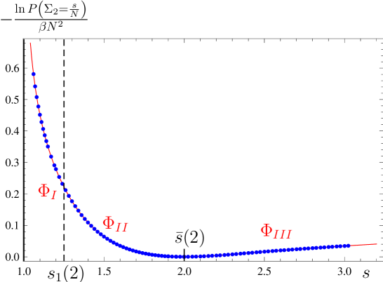
Figure 5: Distribution of $\Sigma_{2}=\sum_{i}\lambda_{i}^{2}$ : the figure shows the rate function $\Phi(s)=-\frac{\ln P\left(\Sigma_{2}=\frac{s}{N}\right)}{\beta N^{2}}$ plotted against $s$ for $N=50$. Analytical predictions (red solid line) are compared with the results (blue points) of Monte Carlo numerical simulations (method 1, as explained in section 6). Our analytical predictions consist of three regimes. For regimes I ($1\leq s<5/4$) and II ($5/4<s<2$), we have plotted the asymptotic expressions of the rate functions in the limit $N\rightarrow\infty$ given in Eqs. (38) and (42). For regime III, we have plotted the analytical prediction for large but finite $N$, using for $\Phi_{III}(s,N)=\Phi(N,s/N)$ (see Eq. (57)) the complete expression of $E$ given in Eq. (61) and $\zeta$ and $t$ (numerical) solutions of Eq. (59) and (60). Indeed, for $N=50$, finite-$N$ corrections to the asymptotic formula in Eq. (51) are important in regime III : the curve of the dominant behavior in $N$ would not fit well the data and the complete expressions are needed. Note in particular that finite-$N$ effects make that the transition between II and III is regularized and appears to be smooth.

4.2.2 Regime II

As $s$ approaches $s_{1}(q)$ from below, the lower bound $L_{1}$ of the density support tends to zero. As the eigenvalues are non-negative, $L_{1}$ cannot be negative. Hence, regime I does not exist for $s>s_{1}(q)$. The critical value $s_{1}(q)$ is the onset of regime II, where the density $\rho_{c}$ has a finite support $]0,L]$ and vanishes only at the upper bound $L$ (see Fig. 3(b)). We will see that regime II is valid for $s_{1}(q)\leq s\leq s_{2}(q,N)$ where $s_{2}(q,N)$ is given in Eq. (23).

Within regime II and for increasing $s$, $\mu_{1}$ increases and becomes positive while $\mu_{2}$ remains positive. The effective potential $V(x)=\mu_{0}+\mu_{1}x+\mu_{2}x^{q}$ has thus a minimum at a smaller and smaller value $x=x^{*}$ that sticks to zero when $\mu_{1}$ becomes positive (see Fig. 4(b)). The charges concentrate close to the origin.

A simple case: $q=2$

Let us begin with the simple case $q=2$. We find the solution of Eq. (31) for $q=2$ by using again the Tricomi formula with $F(x)=V^{\prime}(x)$ (cf Eq. (15)). We are looking for a solution $\rho_{c}$ with finite support $[0,L]$. After imposing $\rho_{c}(L)=0$, we get:

$$\rho_{c}(x)=\frac{1}{\pi}\sqrt{\frac{L-x}{x}}\left[A+Bx\right]\,,$$ (39)

with $A=\mu_{1}+\mu_{2}L$ and $B=2\mu_{2}$.

There are five unkown parameters: the arbitrary constant $C$ in Tricomi’s formula; the upper bound of the density support $L$; the Lagrange multipliers $\mu_{0}$, $\mu_{1}$ and $\mu_{2}$. We also have constraints to enforce. The constraint $\rho_{c}(L)=0$ together with the three constraints $\int\rho_{c}=1$, $\int x\rho_{c}=1$ and $\int x^{2}\rho_{c}=s$ fix the value of the four parameters $C$, $L$, $\mu_{1}$ and $\mu_{2}$. We get $\mu_{0}$ by inserting the final expression of $\rho_{c}$ in Eq. (30) for a special value of $x$, say $x=L$.

We find $C=\int\rho_{c}=1$, $\mu_{1}=8(L-3)/L^{2}$, $\mu_{2}=4(4-L)/L^{3}$ and $\mu_{0}=\ln\left(\frac{L}{4}\right)-\frac{1}{2}-\mu_{1}\frac{L}{4}$. The upper bound of the support $L$ is solution of the equation $L^{2}-12L+16s=0$. Hence $L=2(3\pm\sqrt{9-4s})$. Physically the density $\rho_{c}(x)$ must remain positive for $0<x<L$. It is not difficult to see that this determines $L$:

$$L=L(s)=2(3-\sqrt{9-4s})$$ (40)

The upper bound $L$ increases with $s$ and matches smoothly regime I: $L=2=L_{2}$ at $s=s_{1}(2)=5/4$. The solution of regime II, exists as long as $s<9/4$. However, we shall see that there exists another solution for $s>2$ that is energetically more favorable. This latter solution will yield regime III. The solution of regime II is thus valid only for $5/4<s<2$.

We have seen that $\mu_{1}=8(L-3)/L^{2}$ and $\mu_{2}=4(4-L)/L^{3}$. According to the respective sign of $\mu_{1}$ and $\mu_{2}$, we distinguish three phases for the effective potential $V(x)=\mu_{0}+\mu_{1}x+\mu_{2}x^{2}$:

• $2\leq L<3$ (i.e. $5/4\leq s<27/16$): $\mu_{1}<0$ and $\mu_{2}>0$. The potential $V(x)$ has a minimum at a positive $x=x^{*}=\left(-\mu_{1}\right)/\left(2\,\mu_{2}\right)=L(3-L)/(4-L)$ (as in regime I). $x^{*}$ decreases when $L$ (or $s$) increases and reaches $0$ at $L=3$ (see Fig. 4 (a)).

• $3<L<4$ (i.e. $27/16<s<2$): $\mu_{1}>0$ and $\mu_{2}>0$. The potential is monotonic (increasing) on the real positive axis. It has an absolute minimum at $x=0$ (see Fig. 4 (b)).

• $L>4$ (i.e. $2<s\leq 9/4$): $\mu_{1}>0$ but $\mu_{2}<0$. The potential is not anymore bounded from below. It increases around the origin, reaches a maximum at $x=x^{*}=\left(\mu_{1}\right)/\left(-2\,\mu_{2}\right)=L(L-3)/(L-4)$ and decreases monotonically for $x>x^{*}$ to $-\infty$ (see Fig. 4 (c)). In this phase, the origin is a local minimum and the solution in Eq. (39) is metastable. There is actually a second solution in this phase, where one eigenvalue splits off the sea of the other eigenvalues. This second solution becomes energetically more favorable at $s=s_{2}\approx 2+\frac{2^{4/3}}{N^{1/3}}$. The solution of regime II in Eq. (39) is thus valid only for $s<s_{2}$. For $s>s_{2}$, the second solution dominates: this is regime III.

Finally, the distribution of the purity $\Sigma_{2}$ in regime II is computed by the saddle point method:

$$P\left(\Sigma_{2}=s/N,N\right)\propto\exp\left\{-\beta N^{2}\Phi_{II}(s)\right\}\,,$$ (41)

where the large deviation function $\Phi_{II}=E_{s}\left[\rho_{c}\right]-\frac{1}{4}=-\frac{1}{2}\left[\mu_{1}+\mu_{2}s+\mu_{0}\right]-\frac{1}{4}$ is explicitely given by:

$$\Phi_{II}(s)=-\frac{1}{2}\ln\left(\frac{L}{4}\right)+\frac{6}{L^{2}}-\frac{5}{L}+\frac{7}{8}\,,$$ (42)

with $L=2\left(3-\sqrt{9-4s}\right)$. For large $N$, this solution is valid for $s_{1}(2)<s\leq s_{2}(2,N)$ with $s_{1}(2)=5/4$ and $s_{2}(2,N)\approx 2+\frac{2^{4/3}}{N^{1/3}}\rightarrow 2$ as $N\rightarrow+\infty$ (as we shall see).

At $s=s_{1}=5/4$ (transition between regime I and II), the rate function $\Phi(s)$ has a weak nonanalyticity. It is continuous, $\Phi(5/4)=-\frac{1}{8}+\frac{\ln 2}{2}$, and even twice differentiable: $\frac{d\Phi}{ds}\big{|}_{s=5/4}=-1$ and $\frac{d^{2}\Phi}{ds^{2}}\big{|}_{s=5/4}=4$. However, the third derivative is discontinuous: $\frac{d^{3}\Phi}{ds^{3}}\big{|}_{s=5/4^{-}}=\frac{d^{3}\Phi_{I}}{ds^{3}}\big{|}_{s=5/4}=-32$ but $\frac{d^{3}\Phi}{ds^{3}}\big{|}_{s=5/4^{+}}=\frac{d^{3}\Phi_{II}}{ds^{3}}\big{|}_{s=5/4}=-16$. The minimum of $\Phi$ is reached at $s=2$ within regime II, which gives the mean value of the purity $\langle\Sigma_{2}\rangle\approx 2/N$ (as the distribution is highly peaked around its average for large $N$).

Figure 5 compares our analytical predictions for regimes I and II in Eq. (38) and (42) with numerical data (Monte Carlo simulations): the agreement is very good already for $N=50$.

General case $q>1$

We find the solution $\rho_{c}$ with finite support $[0,L]$ of Eq. (31) for $q>1$ by using again the Tricomi formula with $F(x)=V^{\prime}(x)$ (cf Eq. (15)). After imposing $\rho_{c}(L)=0$, we get the expression of the density:

$$\rho_{c}=\frac{\mu_{1}}{\pi}\sqrt{\frac{L-x}{x}}+\frac{2\mu_{2}qL^{q-1}}{\pi^{3/2}}\frac{\Gamma\left(q+\frac{1}{2}\right)}{\Gamma(q)}\sqrt{\frac{L-x}{x}}\>\,_{2}F_{1}\left(1,1-q,\frac{3}{2},1-\frac{x}{L}\right)\,,$$ (43)

where $\,{}_{2}F_{1}$ is a hypergeometric function $\,{}_{2}F_{1}(a,b,c,z)=\sum_{n=0}^{\infty}\frac{(a)_{n}(b)_{n}}{(c)_{n}}\frac{z^{n}}{n!}$, with $(a)_{n}=a(a+1)...(a+n-1)$ denoting the raising factorial (Pochhammer symbol).

Exactly as for $q=2$, the constraints fix the unknown parameters. We obtain the Lagrange multipliers $\mu_{1}$, $\mu_{2}$ and $\mu_{0}$ as functions of $L$:

$$\mu_{1}=\frac{8(1+q)}{(1-q)L^{2}}-\frac{4q}{L(1-q)}\;\;\;\;\;\textrm{and}\;\;\;\;\;\mu_{2}=\frac{(1+q)}{(1-q)}\>\frac{\sqrt{\pi}\;\Gamma(q)}{\Gamma(q+1/2)}\,\frac{L-4}{L^{q+1}}\,.$$ (44)

and $\mu_{0}=\ln\left(\frac{L}{4}\right)+\mu_{1}\frac{L(1-q)}{2q}-\frac{1}{q}$. The upper bound $L$ (which is a function of $s$) is given by the solution of the equation

$$\left(\frac{1-q}{1+q}\right)L^{q}+4L^{q-1}=\frac{2\sqrt{\pi}\;\Gamma(q+1)}{\Gamma(q+1/2)}\,s\,.$$ (45)

For $q=2$, we recover the simple expressions of the previous subsection.

The function $f:L\rightarrow\left(\frac{1-q}{1+q}\right)L^{q}+4L^{q-1}$ is increasing with $L$ for $0<L<L_{0}$ with $L_{0}=4(1+q)/q$, and decreases for $L>L_{0}$. It is thus maximal at $L=L_{0}$, which implies that $s$ cannot be larger than $s_{0}=s(L=L_{0})$ in this regime. Hence, regime II is not valid for $s>s_{0}$, where $s_{0}=s_{0}(q)=s(L=L_{0})=\frac{\Gamma(q+1/2)}{2\sqrt{\pi}\Gamma(q+2)}\left(\frac{4(1+q)}{q}\right)^{q}$.

Moreover, it can be shown that, for $L<L_{0}/3$ and for $L>L_{0}$, the density $\rho_{c}(x)$ becomes negative for $x$ close to the bounds (close to $0$ for $L<L_{0}/3$, close to $L$ for $L>L_{0}$). This is not physical. Hence, $L$ must belong to the interval $[L_{0}/3,L_{0}]$. Within this range, the function $f$ is monotonic and it increases with $L$. It can thus be inverted and gives $L$ as a single-valued function of $s$: $L=L(s)$. This range $[L_{0}/3,L_{0}]$ corresponds to $s_{1}(q)\leq s\leq s_{0}(q)$, where $s_{1}(q)=s(L=L_{0}/3)$ and $s_{0}=s(L=L_{0})$.

Therefore regime II can exist only for $s_{1}(q)\leq s\leq s_{0}(q)$, where $s_{1}(q)=\frac{\Gamma(q+3/2)}{\sqrt{\pi}\Gamma(q+2)}\left(\frac{4(1+q)}{3q}\right)^{q}$ and $s_{0}(q)=\frac{\Gamma(q+1/2)}{2\sqrt{\pi}\Gamma(q+2)}\left(\frac{4(1+q)}{q}\right)^{q}$. For $q=2$, we recover $s_{1}(2)=5/4$ and $s_{0}(2)=9/4$. However, as in the $q=2$ case, this regime is not valid anymore for $s>s_{2}(q,N)$ given in Eq. (23), where a second solution starts to dominate (regime III).

Finally, we compute the pdf of $\Sigma_{q}$ as a function of $L=L(s)$. We get the pdf by the saddle point method:

$$P\left(\Sigma_{q}=N^{1-q}\,s,N\right)\propto\exp\left\{-\beta N^{2}\Phi_{II}(s)\right\}\,,$$ (46)

where the large deviation function $\Phi_{II}=E_{s}\left[\rho_{c}\right]-\frac{1}{4}$ is explicitely given by:

$$\Phi_{II}(s)=-\frac{1}{2}\ln\left(\frac{L}{4}\right)+\frac{4(1+q)}{qL^{2}}-\frac{2(1+2q)}{qL}+\frac{3q+1}{4q}\,.$$ (47)

The function $L=L(s)$ is the unique solution of Eq. (45) within the range $s_{1}\leq s\leq s_{2}$.

Exactly as for $q=2$, the parameter $\mu_{2}$ (given in Eq. (44)) is positive for $L<4$ ($s<\bar{s}(q)$) and becomes negative for $L>4$ ($s>\bar{s}(q)$). Hence, for all $q>1$ the effective potential $V(x)=\mu_{0}+\mu_{1}x+\mu_{2}x^{q}$ becomes unbounded from below when $L$ exceeds $4$. The solution of regime II is thus metastable in the range $\bar{s}(q)<s<s_{0}(q)$ ($4<L<L_{0}$). Indeed, exactly as for $q=2$, there exists a second solution for $s>\bar{s}(q)$ that becomes energetically more favorable (lower energy) for $s>s_{2}(q)$. This is the onset of regime III. It occurs at $s=s_{2}=\bar{s}$ for very large $N$, more precisely at $s=s_{2}(q,N)\approx\bar{s}(q)+\left[\sqrt{q/2}\,(q-1)\,\bar{s}(q)\right]^{2q/(2q-1)}/N^{(q-1)/(2q-1)}$ for large but finite $N$, as we shall see.

As the distribution of $\Sigma_{q}$ is highly peaked for large $N$, its mean value is given by the most probable value: $\langle\Sigma_{q}\rangle=N^{1-q}\bar{s}(q)$ where $\bar{s}(q)$ minimizes $\Phi(s)$. This minimum $s=\bar{s}(q)=\frac{\Gamma(q+1/2)}{\sqrt{\pi}\Gamma(q+2)}\,4^{q}$ (or equivalently $L(\bar{s})=4$) is reached within regime II and $\Phi_{II}(\bar{s}(q))=0$. For $s$ close to $\bar{s}(q)$, $\Phi_{II}(s)\approx\frac{(s-\bar{s}(q))^{2}}{2\sigma_{q}^{2}}$ where $\sigma_{q}^{2}$ is given in Eq. (21). We conclude that the distribution of $\Sigma_{q}$ has a Gaussian behaviour around its average, as shown in Eq. (20), from which we can read the variance (see Eq. (21)). For example, for $q=2$, we have $\sigma_{2}^{2}=4$ and ${\rm Var}\Sigma_{2}\approx\frac{4}{\beta N^{4}}$.

4.3 Regime III

As $s$ exceeds $\bar{s}(q)$, $\mu_{2}$ becomes negative and the effective potential $V(x)=\mu_{0}+\mu_{1}x+\mu_{2}x^{q}$ is not anymore bounded from below. The solution of regime II becomes metastable. The minimum of the potential at the origin still exists, as $V(x)$ increases for small $x$, but it is a local minimum: $V(x)$ reaches a maximum at $x=x^{*}>0$ and then decreases to $-\infty$ (see Fig. 4(c)). Actually, for $s>\bar{s}(q)$, there exists another solution where one charge splits off the sea of the other $(N-1)$ charges that remain confined close to the origin (in the local minimum of $V$). The maximal eigenvalue (charge) becomes much larger than the other (see Fig. 3(c)). At some point $s=s_{2}(q,N)$ very close to $\bar{s}(q)$ for large $N$, this second solution becomes energetically more favorable than the solution of regime II : this is the onset of regime III. This phase transition occurs at $s=s_{2}(q,N)$ given in Eq. (48). It is reminiscent of the real-space condensation phenomenon observed in a class of lattice models for mass transport, where a single lattice site carries a thermodynamically large mass [38].

4.3.1 Regime III: summary of results

We show in this section that there is an abrupt transition from regime II to III at $s=s_{2}(q,N)$ where:

$$s_{2}(q,N)\approx\bar{s}(q)+\frac{\left[\sqrt{q/2}\,(q-1)\,\bar{s}(q)\right]^{2q/(2q-1)}}{N^{(q-1)/(2q-1)}}\;\;\textrm{for large $N$}\,.$$ (48)

Here, $\bar{s}(q)$ the mean value of $s$ given in Eq. (19). The maximal eigenvalue $t$ suddenly jumps from a value $t\approx T/N$ very close to the upper edge $\zeta$ of the sea of eigenvalues to a value $t\approx\left[s-\bar{s}(q)\right]^{1/q}/N^{1-\frac{1}{q}}$ much larger than the other eigenvalues ($t\gg\zeta$) (see Fig. 3 (c)). This is clearly shown by the good agreement between our predictions and numerical simulations in Fig. 7 for $N=500$ and $N=1000$. The consequence of this phase transition in the Coulomb gas is an abrupt change in the distribution of $\Sigma_{q}$. More precisely, we show that for large $N$ :

$$P\left(\Sigma_{q}=N^{1-q}\,s,N\right)\approx\exp\left\{-\beta N^{1+\frac{1}{q}}\>\Psi_{III}(s)\right\}\;\;\;\textrm{for $s>s_{2}(q,N)$}\,,$$ (49)

where

$$\Psi_{III}(s)=\frac{\left[s-\bar{s}(q)\right]^{1/q}}{2}\,.$$ (50)

The expression of the mean value $\bar{s}(q)$ is given in Eq. (19). For example, for $q=2$, this implies:

$$P\left(\Sigma_{2}=\frac{s}{N},N\right)\approx\exp\left\{-\beta N^{\frac{3}{2}}\>\Psi_{III}(s)\right\}\;\;{\rm with}\;\;\Psi_{III}(s)=\frac{\sqrt{s-2}}{2}\,.$$ (51)

The rate function $\Phi(N,s/N)$ defined by

$$N^{2}\,\Phi(N,s/N)=\left\{\begin{array}[]{ll}N^{2}\,\Phi_{II}(s)&{\rm for}\;\;s<s_{2}\,,\\ N^{1+\frac{1}{q}}\,\Psi_{III}(s)&{\rm for}\;\;s>s_{2}\,,\end{array}\right.$$ (52)

is continuous but its derivative is discontinuous at $s=s_{2}$: for large $N$ we have $\frac{d\Phi}{ds}\big{|}_{s_{2}^{+}}\approx\frac{d\Phi}{ds}\big{|}_{s_{2}^{-}}/(2q)$. At the transition point $s=s_{2}$, there is also a change of concavity of the curve: the rate function in regime II is convex ($\frac{d^{2}\Phi_{II}}{ds^{2}}>0$ for $s<s_{2}$) and has a minimum at $s=\bar{s}$, whereas the rate function in regime III is concave ($\frac{d^{2}\Psi_{III}}{ds^{2}}<0$ for $s>s_{2}$).

Figure 6 shows the transition from regime II to regime III for $q=2$ and $N=1000$: analytical prediction for large $N$ in Eq. (51) compare well with Monte Carlo numerical simulations.

4.3.2 New saddle point

We want to describe the regime where a single charge (the maximal eigenvalue) detaches from the continuum of the other charges. The assumption that all the eigenvalues are close to each other and can be described by a continuous density of states does not hold anymore. The saddle point must be slightly revised.

We write $\lambda_{max}=t$ and label the remaining $(N-1)$ eigenvalues by a continuous density $\rho(\lambda)=\frac{1}{N-1}\sum_{i\neq max}\delta(\lambda-\lambda_{i})$. Physically, as the effective potential has a local minimum at the origin $x=0$, we expect the optimal charge density $\rho_{c}$ to have a finite support over $[0,\zeta]$ with $\zeta<t$ and $\rho_{c}(\zeta)=0$: while one charge (the maximal eigenvalue $t$) splits off the sea, the other charges (the sea) remain confined close to the origin (in the local minimum of $V$, see Fig. 4 (c)).

In this regime, we do not rescale the density (and the energy) by assuming that $\lambda\sim 1/N$. We want indeed to compute the pdf of $\Sigma_{q}=S$ for all $\bar{S}(q)\leq S\leq 1$, where $\bar{S}(q)=N^{1-q}\,\bar{s}(q)$. The effective energy is now a function of both $t$ and $\rho$:

$$E_{S}\left[\rho,t\right]=\!\! - \!\!\frac{(N-1)^{2}}{2}\int_{0}^{\zeta}\int_{0}^{\zeta}d\lambda d\lambda^{\prime}\>\rho(\lambda)\rho(\lambda^{\prime})\,\ln\left|\lambda-\lambda^{\prime}\right|$$ (53)

$$- \!\!(N-1)\int_{0}^{\zeta}d\lambda\>\rho(\lambda)\,\ln\left|t-\lambda\right|+\mu_{0}\left(\int_{0}^{\zeta}d\lambda\>\rho(\lambda)-1\right)$$

$$+ \mu_{1}\left((N-1)\int_{0}^{\zeta}d\lambda\>\lambda\>\rho(\lambda)+t-1\right)$$

$$+ \mu_{2}\left((N-1)\int_{0}^{\zeta}d\lambda\>\lambda^{q}\>\rho(\lambda)+t^{q}-S\right)\,.$$

The dominating configuration is described by the optimal charge density $\rho_{c}$ and the optimal value $t_{c}$ of $t=\lambda_{max}$ such that:

$$\frac{\delta E_{S}}{\delta\rho}\Big{|}_{\rho=\rho_{c},t=t_{c}}=0\;\;{\rm and}\;\;\frac{\partial E_{S}}{\partial t}\Big{|}_{\rho=\rho_{c},t=t_{c}}=0\,.$$ (54)

Taking into account the normalization, we have indeed for large $N$: $P\left(\Sigma_{q}=S,N\right)\approx\frac{\int\mathcal{D}\rho\int dt\;e^{-\beta E_{S}\left[\rho,t\right]}}{\int\mathcal{D}\rho\int dt\;e^{-\beta E\left[\rho,t\right]}}\approx\exp\left\{-\beta\left(E_{S}\left[\rho_{c},t_{c}\right]-E\left[\rho^{*},t^{*}\right]\right)\right\}$, where $E_{S}\left[\rho,t\right]$ is given in Eq. (53) and $E\left[\rho,t\right]$ has the same expression as $E_{S}\left[\rho,t\right]$ but without the last term (the constraint $\sum_{i}\lambda_{i}^{q}=S$). The pair $(\rho^{*},t^{*})$ (resp. $(\rho_{c},t_{c})$) minimizes $E\left[\rho,t\right]$ (resp. $E_{S}\left[\rho,t\right]$). In fact, the normalization is given by the saddle point energy evaluated at $S=\bar{S}$ (the mean value of $S$): $E\left[\rho^{*},t^{*}\right]=E_{S}\left[\rho_{c},t_{c}\right]\Big{|}_{S=\bar{S}}$ (with $\bar{S}=2/N$ for $q=2$). We shall see that for large $N$, we have:

$$E\left[\rho^{*},t^{*}\right]=E_{S}\left[\rho_{c},t_{c}\right]\Big{|}_{S=\bar{S}}\approx N^{2}\left(\frac{\ln N}{2}+\frac{1}{4}\right)\,.$$ (55)

Formally, by analogy with regimes I and II, we can write:

$$P\left(\Sigma_{q}=S,N\right)\approx\exp\left\{-\beta N^{2}\Phi(N,S)\right\}\,,$$ (56)

where we define the rate function $\Phi$ as

$$\Phi(N,S)=\left(E_{S}\left[\rho_{c},t_{c}\right]-E\left[\rho^{*},t^{*}\right]\right)/N^{2}\,.$$ (57)

However, we shall see that the scaling of $\Phi$ with $N$ is different in regime III with respect to the regimes I and II. In regimes I and II, $\Phi$ was independent of $N$ for large $N$: $\Phi(N,s/N)\rightarrow\Phi_{I}(s)$ (resp. $\Phi_{II}(s)$). In regime III, we shall see that: $\Phi(N,s/N)\approx\Psi_{III}(s)/N^{1-\frac{1}{q}}$ for large $N$.

For simplicity, we write $t$ instead of $t_{c}$ in the following.

4.3.3 Case $q=2$

Following the same steps as for regime II, we find that the optimal charge density is explicitly given for $q=2$ by:

$$\rho_{c}(\lambda)=\frac{1}{\pi\,(N-1)}\sqrt{\frac{\zeta-\lambda}{\lambda}}\left[A+B\lambda+\frac{C}{t-\lambda}\right]\,,$$ (58)

with $A=\frac{4}{\zeta^{2}}\left[N\zeta-2+2\sqrt{t(t-\zeta)}\right]$ , $B=\frac{8}{\zeta^{3}}\left[4-N\zeta+\sqrt{\frac{t}{t-\zeta}}\,\left(3\zeta-4t\right)\right]$ and $C=\sqrt{\frac{t}{t-\zeta}}$ , where $\zeta$ and $t=t_{c}$ satisfy:

$$(a) \!\!\!16S+N\zeta^{2}-12\zeta-\sqrt{\frac{t}{t-\zeta}}\left(16t^{2}-20t\zeta+5\zeta^{2}\right)=0\,,$$ (59)

$$(b) \!\!\!\left(8t^{2}-8t\zeta+\zeta^{2}\right)^{2}=8(t-\zeta)\sqrt{t(t-\zeta)}\left(8t-2\zeta-2Nt\zeta+N\zeta^{2}\right)\,.$$ (60)

These equations can be solved numerically for every $\Sigma_{2}=S$. We can also find the solutions analytically for very large $N$.

For $S=\frac{s}{N}$ with $2<s<9/4$, there exist two solutions for the pair $(\zeta,t)$. The first solution is of the form $t\approx\zeta$ with $\zeta\approx O(1/N)$. This is exactly (to leading order in $N$) the solution of regime II (see below, “first solution”). There is also a second solution, where $t\gg\zeta$: the maximal eigenvalue becomes much larger than the other eigenvalues. More precisely, $\zeta\approx O(1/N)$ whereas $t\approx O(1/\sqrt{N})$ for $S\approx O(1/N)$ (see below, “second solution”). We shall see that the first solution (regime II) is valid up to a value $s=s_{2}\approx 2+\frac{2^{4/3}}{N^{1/3}}$ for large $N$, whereas the solution with $t\gg\zeta$ starts to dominate for $s>s_{2}$ (its energy becomes lower): this is regime III.

For $S>\frac{9}{4N}$ ($s>\frac{9}{4}$), there remains only one solution (the second one), where $\zeta=L/N$ and $t\gg\zeta$.

Note that in both cases, for large $N$ (and for $\frac{2}{N}\leq S<1$), the upper bound $\zeta$ remains of the order $\sim O(1/N)$. We shall thus write $\zeta=\frac{L}{N}$ with $L\sim O(1)$. On the other hand, the maximal eigenvalue $t$ scales from $O(1/N)$ (as $S\rightarrow 2/N$) to $O(1)$ (as $S\rightarrow 1^{-}$).

Finally, we compute the saddle point energy as a function of $\zeta=L/N$ and $t$. As finite-size effects (large but finite $N$) are important in this regime, we keep all terms up to order $O(N)$ in the saddle point energy, which gives:

$$E_{S}[\rho_{c},t]=E(\zeta,t)\!\!\!\! = \!\!\!-\frac{(N-1)^{2}}{2}\ln\left[\frac{\zeta}{4}\right]-2N\ln\left[\frac{\sqrt{t}+\sqrt{t-\zeta}}{2}\right]+\frac{1}{2}\ln\left[t(t-\zeta)\right]$$ (61)

$$+\frac{9N^{2}}{8}+\frac{6(1+t^{2})}{\zeta^{2}}-\frac{5(N+t)}{\zeta}+\frac{t}{8(t-\zeta)}$$

$$+\sqrt{\frac{t}{t-\zeta}}\left[-\frac{19N}{4}-\frac{12t}{\zeta^{2}}+\frac{11}{\zeta}+\frac{5Nt}{\zeta}\right]\,,$$

where $\zeta=\zeta(s)$ and $t=t_{c}=t(s)$ are given by Eq. (59) and (60).

The rate function is thus given by $\Phi(N,S)=\left(E_{S}\left[\rho_{c},t\right]-E\left[\rho^{*},t^{*}\right]\right)/N^{2}=\left(E\left[\zeta,t\right]-E\left[\rho^{*},t^{*}\right]\right)/N^{2}$ with $E\left[\zeta,t\right]$ given in Eq. (61).

Scaling $S=s/N$ with $s\sim O(1)$ : first solution $t\approx\zeta$ with $\zeta\sim O(1/N)$ (regime II)

For $S=\frac{s}{N}$ with $s\sim O(1)$ for large $N$, the solution of regime II still exists as long as $s<9/4$ (where $9/4=s_{0}(2)$). We recover this solution from the Eqs.  (59) and (60) with the scaling $t=\frac{T}{N}$ and $\zeta=\frac{L}{N}$ with $T\approx L\sim O(1)$, i.e. the maximal eigenvalue $t$ remains very close to the other eigenvalues ($t\approx\zeta$ for large $N$).

In this limit, equations (59) and (60) indeed give:

$$(a)\;16s+L^{2}-12L \approx 0\,,$$ (62)

$$(b)\;\;\;\;\;(T-L)^{3/2}\;\;\; \approx \frac{L^{5/2}}{8(6-L)}\frac{1}{N}\,.$$ (63)

Equation $(a)$ is the same as Eq. (45) of regime II. To leading order in $N$ (order $N^{2}$), Eq. (61) reduces to:

$$E_{S}[\rho_{c},t]=E(L,t)=-\frac{N^{2}}{2}\ln\left(\frac{L}{4}\right)+6\frac{N^{2}}{L^{2}}-5\frac{N^{2}}{L}+N^{2}\left(\frac{\ln N}{2}+\frac{9}{8}\right)\,.$$ (64)

Therefore, using Eq. (55), we get $\Phi(N,s/N)=\left(E_{S}[\rho_{c},t]-E_{S}[\rho_{c},t]\Big{|}_{s=2}\right)/N^{2}=\Phi(s)$ with $\Phi(s)=-\frac{1}{2}\ln\left(\frac{L}{4}\right)+\frac{6}{L^{2}}-\frac{5}{L}+\frac{7}{8}=\Phi_{II}(s)$. We recover the expression in Eq. (42) of regime II.

However, for $S=s/N>2/N$ there exists a second solution that becomes energetically more favorable at some point $s_{2}\approx 2+\frac{2^{4/3}}{N^{1/3}}$. Therefore regime II is only valid for $5/4<s<s_{2}$.

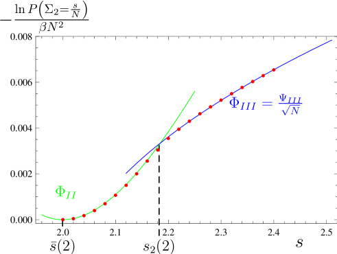
Figure 6: Distribution of $\Sigma_{2}$ : rate function $\Phi=-\ln P\left[\Sigma_{2}=s/N\right]/(\beta N^{2})$ plotted against $s$ for $N=1000$. Analytical results (solid line) are compared with data (red points) of numerical simulations (Monte Carlo, method 2, see section 6). Analytical results here are the rate functions expected in the limit of very large $N$: $\Phi_{II}(s)$ in regime II (green solid line, see Eq. (42)) and $\Phi(N,s/N)\approx\Psi_{III}(s)/\sqrt{N}$ in regime III (blue solid line, see Eq. (51)). The transition between regimes II and III is abrupt, we can see the discontinuity of the derivative of the rate function. It occurs at $s_{2}(q=2,N)\approx 2+\frac{2^{4/3}}{N^{1/3}}-\frac{2^{5/3}\ln N}{3N^{2/3}}\approx 2.18$ for $N=1000$.

Scaling $S=s/N$ with $s\sim O(1)$ : second solution $t\gg\zeta$ (regime III)

For $S=s/N$ with $s>2$, there exists a second solution where one eigenvalue ($\lambda_{\rm max}=t$) becomes much larger than the others : $t\gg\zeta$. In this limit, Eq. (59) and (60) give for large $N$:

$$t\approx\frac{\sqrt{s-2}}{\sqrt{N}}\;\;\;{\rm and}\;\;\;\zeta\approx\frac{4}{N}\left[1+\frac{3-s}{\sqrt{s-2}}\;\frac{1}{\sqrt{N}}\right]\,.$$ (65)

For $S\rightarrow 1$, which implies $s\rightarrow\infty$ as $N\rightarrow\infty$, we find $t\approx\sqrt{\frac{s}{N}}=\sqrt{S}$ and $\zeta\approx\frac{4}{N}\left(1-\sqrt{\frac{s}{N}}\right)\approx\frac{4}{N}(1-t)\;$ as also recovered in Eq. (70).

We can expand the saddle point energy in Eq. (61) replacing $t$ and $\zeta$ by the expressions given in Eq. (65) for large $N$. We obtain:

$$E_{S}\left[\rho_{c},t\right]\approx\frac{\sqrt{s-2}}{2}\,N^{3/2}+N^{2}\left(\frac{\ln N}{2}+\frac{1}{4}\right)-\frac{N}{2}\ln N+O(N)\,\,\,\,\textrm{for large $N$}\,.$$ (66)

Finally, we get $N^{2}\Phi(N,s/N)=E_{s/N}\left[\rho_{c},t\right]-N^{2}\left(\frac{\ln N}{2}+\frac{1}{4}\right)\approx\frac{\sqrt{s-2}}{2}\;N^{3/2}-\frac{N}{2}\ln N+O(N)$ for large $N$ (see Eq. (55)) and the pdf of $\Sigma_{2}$ is thus given for large $N$ by:

$$P\left(\Sigma_{2}=\frac{s}{N},N\right)\approx e^{-\beta N^{3/2}\Psi_{III}(s)}\,,$$ (67)

where $N^{3/2}\Psi_{III}(s)=N^{2}\Phi(N,s/N)$, that is

$$\Psi_{III}(s)=\frac{\sqrt{s-2}}{2}-\frac{\ln N}{2\sqrt{N}}+O\left(\frac{1}{\sqrt{N}}\right)\approx\frac{\sqrt{s-2}}{2}\;\;\;\textrm{for large $N$}\,.$$ (68)

The rate function has a very different behaviour for large $N$ in regime II and III. In regime I and II, we have $P\left(\Sigma_{2}=\frac{s}{N},N\right)\approx e^{-\beta N^{2}\Phi(s)}$, whereas in regime III we have $P\left(\Sigma_{2}=\frac{s}{N},N\right)\approx e^{-\beta N^{3/2}\Psi_{III}(s)}$. For large but finite $N$ and for $s>2$ but very close to $\bar{s}=2$, we have $N^{3/2}\Psi_{III}(s)>N^{2}\Phi_{II}(s)$. Therefore the solution of regime II dominates close to $s=2$. However, the solution of regime III becomes energetically more favorable at some point $s_{2}$ defined by $N^{3/2}\Psi_{III}(s_{2})=N^{2}\Phi_{II}(s_{2})$, that is

$$s_{2}\approx 2+\frac{2^{4/3}}{N^{1/3}}-\frac{2^{5/3}\ln N}{3N^{2/3}}\;\;\textrm{for large $N$}\,.$$ (69)

At $s=s_{2}$, there is an abrupt transition from regime II to III. The maximal eigenvalue $t$ jumps from a value $t\approx\frac{T}{N}$ with $T\sim O(1)$ and $t$ very close to $\zeta$ to a value $t\approx\frac{\sqrt{s-2}}{\sqrt{N}}$ much larger than the other eigenvalues ($t\gg\zeta$). The rate function is continuous but its derivative is discontinuous: $N^{2}\frac{d\Phi_{II}}{ds}\Big{|}_{s=s_{2}^{-}}\approx\frac{N^{5/3}}{2^{2/3}}$, whilst $N^{3/2}\frac{d\Psi_{III}}{ds}\Big{|}_{s=s_{2}^{+}}\approx\frac{N^{5/3}}{4\,2^{2/3}}$ for large $N$. At the transition point $s=s_{2}$, there is also a change of concavity of the curve: the rate function in regime II is convex ($\frac{d^{2}\Phi_{II}}{ds^{2}}>0$ for all $s<9/4$) and has a minimum at $s=\bar{s}=2$, whereas the rate function in regime III is concave ($\frac{d^{2}\Psi_{III}}{ds^{2}}<0$ for all $s>2$).

Scaling $\Sigma_{2}=S\approx O(1)$ and limit $S\rightarrow 1$ (unentangled state)

In the far-right tail of the distribution $\Sigma_{2}=S\approx O(1)$ ($S\gg s/N$, $S\leq 1$) and the maximal eigenvalue $t\approx O(1)$ whereas $\zeta$ (and all the other eigenvalues) remain of order $O(1/N)$. In this limit, equations (59) and (60) become:

$$S\approx t^{2}\;\;{\rm and}\;\;L\approx 4(1-t)\;\;{\rm as}\;t\approx O(1)\,.$$ (70)

The saddle point energy in Eq. (61) reduces to: $E_{S}\left[\rho_{c},t\right]\approx-\frac{N^{2}}{2}\ln\left(1-t\right)+N^{2}\left(\frac{\ln N}{2}+\frac{1}{4}\right)-N\ln N+O(N)$ as $S\approx O(1)$ with $t=\sqrt{S}$. Using Eq. (55), we get an explicit expression for the rate function $\Phi(N,S)=\left(E_{S}\left[\rho_{c},t_{c}\right]-E\left[\rho^{*},t^{*}\right]\right)/N^{2}$ for large $N$:

$$\Phi(N,S)\approx\frac{\left(E_{S}\left[\rho_{c},t\right]-N^{2}\left(\frac{\ln N}{2}+\frac{1}{4}\right)\right)}{N^{2}}\approx-\frac{1}{2}\ln\left(1-\sqrt{S}\right)\equiv\Phi_{III}(S)\,.$$ (71)

We conclude that

$$P\left(\Sigma_{2}=S,N\right)\approx e^{-\beta N^{2}\Phi_{III}(S)}\approx\left(1-\sqrt{S}\right)^{\frac{\beta N^{2}}{2}}\;\;\textrm{for large $N$, fixed $S$}\,.$$ (72)

The difference of scaling with respect to regimes I and II comes from the scaling of $\Sigma_{2}$: in regimes I (resp. II), we had $\Phi(N,s/N)\rightarrow\Phi_{I}(s)$ (resp. $\Phi_{II}(s)$) for large $N$, whereas here we have: $\Phi(N,S)\rightarrow\Phi_{III}(S)$ for large $N$ and fixed $S\approx O(1)$. As $S=s/N$ with fixed $s$ and large $N$, which corresponds to the limit $S\rightarrow 0$ in this scaling, we find $N^{2}\Phi_{III}(S)\approx N^{3/2}\,\sqrt{s}/2$ which is also the limit $s\rightarrow\infty$ of $N^{3/2}\Psi_{III}(s)$. The right tail (where $S\approx O(1/N)$) and the far-right tail (where $S\approx O(1)$) of the distribution match smoothly.

As $\Sigma_{2}=S$ tends to its maximal value $1$, the maximal eigenvalue $t\rightarrow 1$ and $L\rightarrow 0$. At $S=1$, only one eigenvalue, the maximal one $\lambda_{max}=t$, is nonzero (and equal to one). This corresponds to an unentangled state (situation (i)). The probability of an unentangled state (i.e. $\Sigma_{2}\rightarrow 1$) is thus vanishingly small for large $N$.

Figure 7: Maximal eigenvalue $\lambda_{\rm max}=t$ corresponding to a fixed value of the purity $\Sigma_{2}=s/N$ plotted against $s$ for different values of $N$. Analytical predictions (solid lines) are compared with numerical simulations (points : Monte Carlo data, method 2 with density). The theory predicts for large $N$ a sudden jump of $t$ from a value $t\approx\zeta=L(s)/N$ with $L(s)=2(3-\sqrt{9-4s})$ (within regime II, $s<s_{2}$) to a much larger value $t\approx\frac{\sqrt{s-2}}{\sqrt{N}}$ (regime III, $s>s_{2}$). We clearly see this jump in numerical simulations for $N=500$ at $s_{2}\approx 2.23$ and $N=1000$ at $s_{2}\approx 2.18$. For $N=50$, finite-size corrections to the large $N$ asymptotics are considerable enough to smear the jump in $t$. Because of the choice of scaling on the plot, $tN$ as a function of $s$, the plots of the maximal eigenvalue in regime II are expected to be the same for different $N$ (for large $N$), whereas the plots for regime III differ by a factor $\sqrt{N}$.

4.3.4 General $q>1$

Using again Tricomi’s theorem and imposing the constraints $\int\rho_{c}=1$ and $\rho_{c}(\zeta)$, we find that the optimal charge density for the $N-1$ smallest eigenvalues is given by:

$$\rho_{c}(\lambda)=\frac{1}{\pi(N-1)}\sqrt{\frac{\zeta-\lambda}{\lambda}}\,\left[A+B\>\,_{2}F_{1}\left(1,1-q,\frac{3}{2},1-\frac{\lambda}{\zeta}\right)+\frac{C}{t-\lambda}\right]\,,$$ (73)

where $A=\mu_{1}$, $B=\mu_{2}2q\zeta^{q-1}\frac{\Gamma(q+1/2)}{\sqrt{\pi}\Gamma(q)}$ and $C=\sqrt{\frac{t}{t-\zeta}}$ and $\,{}_{2}F_{1}$ is a hypergeometric function $\,{}_{2}F_{1}(a,b,c,z)=\sum_{n=0}^{\infty}\frac{(a)_{n}(b)_{n}}{(c)_{n}}\frac{z^{n}}{n!}$, with $(a)_{n}=a(a+1)...(a+n-1)$ denoting the raising factorial (Pochhammer symbol). The Lagrange multipliers $\mu_{1}$ and $\mu_{2}$ are given by:

$$\mu_{1}\!\!\! = \!\!\!\frac{4}{(q-1)\zeta^{2}}\left[qN\zeta-2(q+1)+\sqrt{\frac{t}{t-\zeta}}\left\{(2q+2)t-(2q+1)\zeta\right\}\right]\,,$$

$$\mu_{2}\!\!\! = \!\!\!\frac{\sqrt{\pi}\Gamma(q+2)}{\zeta^{q+1}\Gamma(q+1/2)q(q-1)}\left[4-N\zeta+\sqrt{\frac{t}{t-\zeta}}\left\{3\zeta-4t\right\}\right]\,,$$ (74)

where $\zeta$ and $t$ are solutions of the following system of equations:

$$(a) \!\!\!\!S-t^{q}=\frac{\zeta^{q-1}\Gamma(q+1/2)}{\sqrt{\pi}\Gamma(q+1)}\left\{2-\frac{N\zeta}{2}\left(\frac{q-1}{q+1}\right)+\sqrt{\frac{t}{t-\zeta}}\left[\zeta\left(\frac{3q+1}{2q+2}\right)\right.\right.$$ (76)

$$\;\;\;\;\;\;\;\;\;\left.\left.-2t\right]\right\}+\sqrt{\frac{t}{t-\zeta}}\>\frac{\zeta^{q+1}\Gamma(q+1/2)}{2t\sqrt{\pi}\Gamma(q+2)}\;_{2}F_{1}\left(1,q+\frac{1}{2},2+q,\frac{\zeta}{t}\right)\,,$$

$$(b) \!\!\!\!\!\mu_{1}\sqrt{\frac{t-\zeta}{t}}\>+q\mu_{2}t^{q-1}=\frac{\zeta}{2t(t-\zeta)}+$$

$$\mu_{2}\frac{\zeta^{q}\Gamma(q+\frac{1}{2})}{t\sqrt{\pi}\Gamma(q)}\,_{2}F_{1}\left(1,q,q+1,\frac{\zeta}{t}\right)\,,\hskip 28.45274pt$$

with $\mu_{1}=\mu_{1}(\zeta,t)$ and $\mu_{2}=\mu_{2}(\zeta,t)$ given in Eq. (74).

These equations can be solved analytically for large $N$ and the solutions are qualitatively the same as for $q=2$.

For $S=N^{1-q}\,s$ with $\bar{s}(q)<s<s_{0}(q)$ (where $s_{0}(q)=\frac{\Gamma(q+1/2)}{2\sqrt{\pi}\Gamma(q+2)}\left(\frac{4(1+q)}{q}\right)^{q}$, see regime II), there exist two different solutions for the pair $(\zeta,t)$. The first solution is of the form $t\approx\zeta$ with $\zeta\approx O(1/N)$. This is exactly (to leading order in $N$) the solution of regime II (see below, “first solution”). There is also a second solution with $t\gg\zeta$, more precisely $\zeta=L/N$ with $L\sim O(1)$ and $t\approx O(1/N^{1-1/q})$ for $S\approx N^{1-q}\,s$, and $\zeta\approx O(1/N)$ (see below, “second solution”). For $s$ close to $\bar{s}(q)$, the first solution dominates (regime II), but at some point $s=s_{2}(q,N)>\bar{s}(q)$ given in Eq. (80), the second solution, with $t\gg\zeta$, starts to dominate (its energy becomes lower): this is regime III.

For $S>N^{1-q}\,s_{0}(q)$, i.e. $s>s_{0}$, only the second solution remains: the upper bound of the density support scales as $\zeta=L/N$ with $L\sim O(1)$ while the maximal eigenvalue is much larger than all other eigenvalues: $t\gg\zeta$.

In both cases (as for $q=2$), for large $N$ the upper bound $\zeta$ remains of order $\sim O(1/N)$ ($\zeta\sim\lambda_{\rm typ}$). We shall thus write $\zeta=\frac{L}{N}$ with $L\sim O(1)$. On the other hand (as for $q=2$), the maximal eigenvalue $t$ scales from $O(1/N)$ (as $S\rightarrow N^{1-q}\bar{s}(q)$) to $O(1)$ (as $S\rightarrow 1^{-}$).

Scaling $S=N^{1-q}\,s$ with $s\sim O(1)$ : first solution $t\approx\zeta$ with $\zeta\sim O(1/N)$ (regime II)

For $S=N^{1-q}\,s$ with $s\sim O(1)$ for large $N$, the solution of regime II still exists as long as $s<s_{0}(q)$. We recover this solution from the Eq. (76) and (76) with the scaling $t=\frac{T}{N}$ and $\zeta=\frac{L}{N}$ with $T\approx L\sim O(1)$, where the maximal eigenvalue $t$ remains very close to the other eigenvalues ($t\approx\zeta$ for large $N$), it does not play a special role. Using Eq. (55), we finally get $\Phi(N,s/N)=\left(E_{S}[\rho_{c},t]-E_{S}[\rho_{c},t]\Big{|}_{s=2}\right)/N^{2}=\Phi_{II}(s)$, the same expression as in Eq. (47) of regime II.

However, for $s>\bar{s}(q)$ there exists a second solution that becomes energetically more favorable at some point $s_{2}(q,N)$. Therefore regime II is only valid for $s_{1}<s<s_{2}$.

Scaling $S=N^{1-q}\,s$ with $s\sim O(1)$ : second solution $t\gg\zeta$ (regime III)

For $S=N^{1-q}\,s$ with $s>\bar{s}(q)$, there exists a second solution where one eigenvalue ($\lambda_{\rm max}=t$) becomes much larger than the other eigenvalues : $t\gg\zeta$. In this limit, Eq. (76) and (76) give for large $N$:

$$t\approx\frac{\left[s-\bar{s}(q)\right]^{1/q}}{N^{1-1/q}}\;\;\;{\rm and}\;\;\;\zeta\approx\frac{4}{N}\left[1-\left\{\frac{s-\bar{s}(q)(1+q)/2}{\left[s-\bar{s}(q)\right]^{1-1/q}}\right\}\,\frac{1}{N^{1-1/q}}\right]\,.$$ (77)

For $S\rightarrow 1$, which implies $s\rightarrow\infty$ as $N\rightarrow\infty$, we find $t\approx s^{1/q}\,N^{1/q-1}=S^{1/q}$ and $\zeta\approx\frac{4}{N}(1-t)\;$.

We can compute the saddle point energy in this limit replacing $t$ and $\zeta$ by the expressions given in Eq. (77) for large $N$. Finally, we get $N^{2}\Phi(N,s/N)=E_{S}\left[\rho_{c},t\right]-N^{2}\left(\frac{\ln N}{2}+\frac{1}{4}\right)\approx N^{1+\frac{1}{q}}\,\frac{\left[s-\bar{s}(q)\right]^{1/q}}{2}$ for large $N$ (see Eq. (55)) and the pdf of $\Sigma_{q}$ is thus given for large $N$ by:

$$P\left(\Sigma_{q}=N^{1-q}\,s,N\right)\approx\exp\left\{-\beta N^{1+\frac{1}{q}}\,\Psi_{III}(s)\right\}\,,$$ (78)

where

$$\Psi_{III}(s)=\frac{\left[s-\bar{s}(q)\right]^{1/q}}{2}\;\;\;\textrm{for large $N$}\,.$$ (79)

The solution of regime III becomes energetically more favorable, that is $N^{1+\frac{1}{q}}\Psi_{III}(s)<N^{2}\Phi_{II}(s)$, at some point $s_{2}(q,N)$ defined by $N^{1+\frac{1}{q}}\,\Psi_{III}(s_{2})=N^{2}\Phi_{II}(s_{2})$. Therefore

$$s_{2}(q,N)\approx\bar{s}(q)+\frac{\left[\sqrt{q/2}\,(q-1)\,\bar{s}(q)\right]^{2q/(2q-1)}}{N^{(q-1)/(2q-1)}}\;\;\textrm{for large $N$}\,.$$ (80)

At $s=s_{2}$, there is an abrupt transition from regime II to III. The maximal eigenvalue $t$ jumps from a value $t\approx\frac{T}{N}$ with $T\sim O(1)$ and $t$ very close to $\zeta$ to a value $t\approx\frac{\left[s-\bar{s}(q)\right]^{1/q}}{N^{1-1/q}}$ much larger than the other eigenvalues ($t\gg\zeta$). The rate function $\Phi(N,s/N)$ given by

$$N^{2}\,\Phi(N,s/N)=\left\{\begin{array}[]{ll}N^{2}\,\Phi_{II}(s)&{\rm for}\;\;s<s_{2}\,,\\ N^{1+\frac{1}{q}}\,\Psi_{III}(s)&{\rm for}\;\;s>s_{2}\,,\end{array}\right.$$ (81)

is continuous but its derivative is discontinuous. For large $N$, we have indeed $N^{2}\,\frac{d\Phi}{ds}\big{|}_{s_{2}^{-}}\approx N^{\frac{3q-1}{2q-1}}\,\left\{(q-1)\sqrt{q/2}\>\bar{s}(q)\right\}^{\frac{2-2q}{2q-1}}$, whilst $\frac{d\Phi}{ds}\big{|}_{s_{2}^{+}}\approx\frac{d\Phi}{ds}\big{|}_{s_{2}^{-}}/(2q)$. At the transition point $s=s_{2}$, there is also a change of concavity of the curve: the rate function in regime II is convex ($\frac{d^{2}\Phi_{II}}{ds^{2}}>0$) and has a minimum at $s=\bar{s}$, whereas the rate function in regime III is concave ($\frac{d^{2}\Psi_{III}}{ds^{2}}<0$).

5 Distribution of the Renyi entropy $S_{q}$

In section 4, we have computed the full distribution of $\Sigma_{q}=\sum_{i=1}^{N}\lambda_{i}^{q}$ for large $N$. A simple change of variable gives the distribution of the Renyi entropy $S_{q}=\frac{1}{1-q}\ln\left[\sum_{i}\lambda_{i}^{q}\right]=\frac{1}{1-q}\ln\left[\Sigma_{q}\right]$. The scaling $\Sigma_{q}=N^{1-q}s$ for large $N$ implies $S_{q}=\ln N-\frac{\ln s}{q-1}$. This means that typical values of $S_{q}$ will be of order $S_{q}\approx\ln N-z$ with $z\approx O(1)$ for large $N$. The parameter $z=\frac{\ln s}{q-1}$ is nonnegative and its minimum $z=0$ corresponds to $S_{q}=\ln N$, which corresponds to the maximally entangled state.

The distribution of the entropy is thus given for large $N$ by:

$$P\left(S_{q}=\ln N-z\right)\approx\left\{\begin{array}[]{ll}\exp\left\{-\beta N^{2}\>\phi_{I}(z)\right\}&{\rm for}\;\;0<z\leq z_{1}(q)\,,\\ &\\ \exp\left\{-\beta N^{2}\>\phi_{II}(z)\right\}&{\rm for}\;\;z_{1}(q)<z\leq z_{2}(q)\,,\\ &\\ \exp\left\{-\beta N^{1+\frac{1}{q}}\;\psi_{III}(z)\right\}&{\rm for}\;\;z>z_{2}(q)\,.\end{array}\right.$$ (82)

The three regimes are the same as for $\Sigma_{q}$. The rate functions $\phi_{I}$, $\phi_{II}$ and $\psi_{III}$ are simply obtained from the rate functions $\Phi_{I}$, $\Phi_{II}$ and $\Psi_{III}$ for the distribution of $\Sigma_{q}$ (see Eq. (18)) by the change of variable $s=\exp\left[(q-1)z\right]$, e.g. $\phi_{I}(z)=\Phi_{I}\left(e^{(q-1)z}\right)$. Explicit expressions of the functions $\Phi_{I}$ and $\Phi_{II}$ are given in Eq. (38) and (42) for $q=2$, and in Eq. (47) for a general $q>1$; an explicit expression of $\Psi_{III}$ is given in Eq. (50) for a general $q>1$ (and in Eq. (51) for $q=2$).

The critical points are given by

$$z_{1}(q)=\frac{\ln s_{1}(q)}{q-1}\;\;{\rm and}\;\;z_{2}(q,N)=\frac{\ln s_{2}(q,N)}{q-1}\,,$$ (83)

where $s_{1}$ and $s_{2}$ are the critical points for $\Sigma_{q}$ (see Eqs. (22) and (23)).

The distribution of the entropy $S_{q}$ has the same qualitative behaviour as that of $\Sigma_{q}$ : it is a highly peaked distribution with Gaussian behaviour around the mean value and non-Gaussian tails. Again, the average value of $S_{q}$ coincides with the most probable value for large $N$, $\langle S_{q}\rangle\approx\ln N-\bar{z}(q)$ where $\bar{z}(q)$ is the minimum of $\phi_{II}$:

$$\langle S_{q}\rangle\approx\ln N-\bar{z}(q)\;\;{\rm with}\;\;\bar{z}(q)=\frac{\ln\bar{s}(q)}{q-1}=\frac{1}{q-1}\,\ln\left[\frac{\Gamma(q+1/2)}{\Gamma(q+2)}\,\frac{4^{q}}{\sqrt{\pi}}\right]\,.$$ (84)

The rate function $\phi_{II}(z)$ has a quadratic behaviour around $z=\bar{z}(q)$: $\phi_{II}(z)\approx\frac{(z-\bar{z}(q))^{2}}{q}$. Therefore, the distribution of the entropy $S_{q}$ has a Gaussian behaviour around its average:

$$P\left(S_{q}=\ln N-z\right)\approx\exp\left\{-\beta N^{2}\frac{(z-\bar{z}(q))^{2}}{q}\right\}\;\;\textrm{for}\;\;z\approx\bar{z}(q)\,,$$ (85)

which gives the variance of the distribution:

$${\rm Var}\,S_{q}\approx\frac{q}{2\beta N^{2}}\;\;\textrm{for large $N$}\,.$$ (86)

5.1 Limit $q\rightarrow 1^{+}$ : von Neumann entropy

As $q\rightarrow 1^{+}$, the Renyi entropy $S_{q}$ tends to the von Neumann entropy $S_{\rm VN}=-\sum_{i}\lambda_{i}\ln\lambda_{i}$. The limit $q\rightarrow 1$ is singular for the distribution of $\Sigma_{q}$ : because of the constraint $\Sigma_{1}=\sum_{i}\lambda_{i}=1$, the distribution tends to a Dirac-$\delta$ function. The variance tends to zero ($\sigma_{q}^{2}\rightarrow 0$) and the mean value $\bar{s}(q)$ as well as the critical point $s_{1}(q)$ and $s_{2}(q)$ tend to $1$. However, due to the factor $1/(1-q)$ in the definition of $S_{q}$, the limit $q\rightarrow 1$ is not at all singular for the entropy $S_{q}$. Taking this limit only requires to be careful. For $S_{\rm VN}$ (as for $S_{q}$ for $q>1$), there are three regimes in the distribution:

$$P\left(S_{\rm VN}=\ln N-z\right)\approx\left\{\begin{array}[]{ll}\exp\left\{-\beta N^{2}\>\phi_{I}(z)\right\}&{\rm for}\;\;0<z\leq z_{1}\,,\\ &\\ \exp\left\{-\beta N^{2}\>\phi_{II}(z)\right\}&{\rm for}\;\;z_{1}<z\leq z_{2}\,,\\ &\\ \exp\left\{-\beta\frac{N^{2}}{\ln N}\;\phi_{III}(z)\right\}&{\rm for}\;\;z>z_{2}\,,\end{array}\right.$$ (87)

where $\phi_{II}$ and $\phi_{III}$ are respectively given in Eqs. (90) and (94). For $q\rightarrow 1$, we get: $\bar{z}(q)=\frac{\ln\bar{s}(q)}{q-1}\rightarrow 1/2$ (where $\bar{z}(q)$ is given in Eq. (84)). We thus recover the already known mean value of the von Neumann entropy (see [3]) in the case $c=1$ ($M\approx N$):

$$\langle S_{\rm VN}\rangle\approx\ln N-\frac{1}{2}\;\;\textrm{for large $N$}\,.$$ (88)

The critical points separating the three regimes are given by (limit $q\rightarrow 1$ in Eqs. (83) and (22)):

$$z_{1}=\frac{2}{3}-\ln\frac{3}{2}\approx 0.26\;\;{\rm and}\;\;z_{2}\approx\bar{z}=\frac{1}{2}\,.$$ (89)

We easily obtain the expression of the rate function $\phi_{II}$ in regime II by taking the limit $q\rightarrow 1$. We get:

$$\phi_{II}(z)=-\frac{1}{2}\ln\left(\frac{L}{4}\right)+\frac{8}{L^{2}}-\frac{6}{L}+1\,,$$ (90)

where $L=L(z)$ is the solution of (limit $q\rightarrow 1$ in Eq. (45))

$$\ln\left(\frac{L}{4}\right)-\frac{L}{8}+1=z\,.$$ (91)

For large $N$, the mean value corresponds to the minimum of $\phi_{II}$. The quadratic approximation of $\phi_{II}$ around this minimum $z\approx\bar{z}$ gives the Gaussian behaviour of the pdf of $S_{\rm VN}$ around its average and thus the variance in the large $N$ limit:

$$\langle S_{\rm VN}\rangle\approx\ln N-\bar{z}\;\;{\rm with}\;\;\bar{z}=\frac{1}{2}\;\;{\rm and}\;\;{\rm Var}\,S_{\rm VN}\approx\frac{1}{2\beta N^{2}}\,.$$ (92)

The limit $q\rightarrow 1$ for the regime III is a bit more subtle. We would expect the rate function to be of the form $N^{2}\psi_{III}(z)$, but $\psi_{III}=\Psi_{III}(e^{(q-1)z})$ (in Eq. (50)) vanishes as $q\rightarrow 1$. The rate function actually scales as $N^{2}/\ln N$ (rather than $N^{2}$ as one could naïvely expect). This can be shown by a more detailed analysis of the equations (76) and (76) in the limit $q\rightarrow 1$. The solution $t\gg\zeta$ is actually given for $q\rightarrow 1$ by:

$$t\approx\frac{z-1/2}{\ln N}\;\;{\rm and}\;\;\zeta\approx\frac{4}{N}\left(1+\frac{1-z}{\ln N}\right)\,.$$ (93)

The saddle point energy can be computed in this limit. We finally find:

$$-\ln P(S_{\rm VN}=\ln N-z)\approx\beta\frac{N^{2}}{\ln N}(z-1/2)\,;\quad\phi_{III}(z)=z-\frac{1}{2}\,.$$ (94)

5.2 Limit $q\rightarrow\infty$ : maximal eigenvalue

As $q\rightarrow\infty$ the Renyi entropy $S_{q}$ tends to $-\ln\lambda_{\rm max}$ where $\lambda_{\rm max}$ is the maximal eigenvalue. Again, the limit is singular for the distribution of $\Sigma_{q}$ but not for $S_{q}$. There are the same three regimes in the distribution of $\lambda_{\rm max}$ for large $N$ as in the distribution of the Renyi entropy.

For large $N$, the typical scaling is $S_{q}\approx\ln N-z$, thus $-\ln\lambda_{\rm max}\approx\ln N-z$ or $\lambda_{\rm max}\approx\frac{e^{z}}{N}$. Setting $t=e^{z}$, we have $\lambda_{\rm max}=t/N$. In particular, the mean value is given by $\bar{t}/N$ where $\bar{t}=\lim_{q\rightarrow\infty}\exp(\bar{z}(q))=\lim_{q\rightarrow\infty}\left[\bar{s}(q)\right]^{\frac{1}{q-1}}=4$, implying

$$\langle\lambda_{\rm max}\rangle\approx\frac{4}{N}\,.$$ (95)

The first critical point is $t_{1}=\lim_{q\rightarrow\infty}\left[s_{1}(q)\right]^{\frac{1}{q-1}}=4/3$. The second critical point is $t_{2}=\bar{t}=4$. The three regimes in the distribution of the maximal eigenvalue are the following:

$$P\left(\lambda_{\rm max}=\frac{t}{N}\right)\approx\left\{\begin{array}[]{ll}e^{-\beta N^{2}\chi_{I}(t)}&{\rm for}\;\;1<t\leq 4/3\;\;\textrm{(reg. {\bf I})}\,,\\ &\\ e^{-\beta N^{2}\chi_{II}(t)}&{\rm for}\;\;4/3<t\leq 4\;\;\textrm{(reg. {\bf II})}\,,\\ &\\ e^{-\beta N\chi_{III}(t)}&{\rm for}\;\;t>4\;\;\textrm{(reg. {\bf III})}\,.\end{array}\right.$$ (96)

The rate functions can be explicitely computed. The rate function in regime I is given by:

$$\chi_{I}(t)=-\frac{1}{2}\ln(t-1)\;\;\;\;{\rm for}\;\;1<t\leq 4/3\,.$$ (97)

In regime II, we find:

$$\chi_{II}(t)=4\frac{(1-t)}{t^{2}}-\frac{1}{2}\ln\left(\frac{t}{4}\right)+\frac{3}{4}\;\;\;\;{\rm for}\;\;4/3<t\leq 4\,.$$ (98)

Finally, in regime III the maximal eigenvalue detaches from the sea of the other eigenvalues and we get:

$$\chi_{III}(t)=\frac{\sqrt{t(t-4)}}{2}-2\ln(\sqrt{t}+\sqrt{t-4})+2\ln 2\;\;\;\;\textrm{for $t>4$}\,.$$ (99)

Again, at the first critical point $t_{1}=4/3$, the rate function $\chi$ is continuous and twice differentiable, but its third derivative is discontinuous: $\frac{d^{3}\chi_{I}}{dt^{3}}=-27$ but $\frac{d^{3}\chi_{II}}{dt^{3}}=-999/64$. The average value $\bar{t}=4$ is the minimum of $\chi_{II}$. At the second critical point $t_{2}=4$, the rate function is continuous but not differentiable.

Exactly as we did for $\Sigma_{q}$, we can also consider the regime where $\lambda_{\rm max}=T$ ($T\gg t/N$): the far-right tail of the distribution. We find:

$$P\left(\lambda_{\rm max}=T\right)\approx e^{-\beta N^{2}\chi_{+}(T)}\;\;\chi_{+}(T)=-\frac{1}{2}\ln(1-T)\;\;{\rm for}\;\;0<T<1\,,$$ (100)

which matches smoothly regime III. We have indeed: $N\chi_{III}(t)\approx N\frac{t}{2}$ as $t\rightarrow\infty$ and $N^{2}\chi_{+}(t)\approx N^{2}\frac{T}{2}\approx N\frac{t}{2}$ as $T\rightarrow 0$ with $T=t/N$.

Ideas of proof

Regimes II and III can be derived by taking carefully the limit $q\rightarrow\infty$ (directly in the expression of the rate function for regime II but more carefully for regime III). The distribution of $\lambda_{\rm max}$ can also be computed directly (without taking the limit $q\rightarrow\infty$). This gives the same results for regimes II and III and gives also an explicit expression for regime I (where the rate function is not explicitely known for a general $q>1$). We can actually calculate the cumulative distribution ${\rm Prob}\left(\lambda_{\rm max}\leq Z\right)$ by the same Coulomb gas method as before. This is indeed easier to compute because the probability that $\lambda_{\rm max}\leq Z$ is the probability that all the eigenvalues $\lambda_{i}$ are smaller than $Z$. We can thus compute this probability with the Coulomb gas method, with a continuous density $\rho(x)=1/N\,\sum_{i}\delta(x-\lambda_{i}N)$ and with the constraint that no eigenvalue exceeds $Z$:

$$P\left(\lambda_{\rm max}\leq Z\right)\propto\int\mathcal{D}\rho\,e^{-\beta N^{2}E_{Z}\left[\rho\right]}\,.$$ (101)

The energy reads

$$E_{Z}\left[\rho\right] = -\frac{1}{2}\int_{0}^{Z}\int_{0}^{Z}\,\rho(x)\rho(x^{\prime})\ln|x-x^{\prime}|\,dx\,dx^{\prime}+\mu_{0}\left(\int_{0}^{Z}\rho(x)dx-1\right)$$ (102)

$$+\mu_{1}\left(\int_{0}^{Z}x\rho(x)dx-1\right)\,,$$

where the Lagrange multipliers $\mu_{0}$ and $\mu_{1}$ enforce the two constraints $\int\rho=1$ (normalization of the density) and $\int x\rho=1$ (unit sum of the eigenvalues: $\sum_{i}\lambda_{i}=1$). The saddle point method gives:

$$P\left(\lambda_{\rm max}\leq Z\right)\propto\,e^{-\beta N^{2}E_{Z}\left[\rho_{c}\right]}\,,$$ (103)

where $\rho_{c}$ minimizes the effective energy $E_{Z}$. This yields regimes I and II. Exactly as for $S_{q}$, in regime III, the maximal eigenvalue detaches from the sea of the other charges (eigenvalues), it must be taken into account separately from the continuous density of the other eigenvalues.

In regime I, the optimal charge density has a finite support $[L_{1},L_{2}]$ and vanishes at $L_{1,2}$ (exactly as for $\Sigma_{q}$). We get the rate function $\chi_{I}$ in Eq. (97).

In regime II, the optimal charge density has a finite support $]0,L]$, vanishes at $L$ but diverges at the origin with a square root divergence (exactly as for $\Sigma_{q}$). We get the rate function $\chi_{II}$ in Eq. (98). This expression can also be obtained by taking the limit $q\rightarrow\infty$ of the expression in Eq. (47) of $\Phi_{II}$, valid for a general $q$ (for $\Sigma_{q}$).

In regime III, the maximal eigenvalue is much larger than the others and we get $\chi_{III}$ in Eq. (99). The limit $q\rightarrow\infty$ in the rate function $\psi_{III}$ for a general $q$ gives: $\psi_{III}\longrightarrow t/2$. This is actually equal to $\chi_{III}(t)$ only in the limit $t\rightarrow\infty$, but not for all $t>4$. For $q>1$, regime III is characterized by $t\approx T/N^{1-\frac{1}{q}}\gg\zeta$ as $\zeta\approx L/N$, which becomes $t\approx T/N>\zeta$ in the limit $q\rightarrow\infty$. The maximal eigenvalue is larger than the other eigenvalues, but not much larger. We cannot anymore assume $t\gg\zeta$ in the computation of the energy. We must compute carefully the energy $E_{S}\left[\rho_{c},t\right]$ in this limit. For this computation, we use the complete expression of $E_{S}$: for $q=2$, this expression was given in Eq. (61); for a general $q$, we have a similar but more complicated expression. We use this expression in the limit where $t$ and $\zeta$ are both of order one (with $t>\zeta$) and where $q\rightarrow\infty$. We finally get $\chi_{III}(t)$ as given in Eq. (99).

5.2.1 Typical fluctuations around the average: Tracy-Widom distribution

We have seen that the average value of the maximal eigenvalue, in the large $N$ limit, is given by $\langle\lambda_{\rm max}\rangle\approx 4/N$. Of course, $\lambda_{\rm max}$ fluctuates around this average from sample to sample. The Coulomb gas method presented in this subsection captures fluctuations $\sim O(1/N)$ around this mean, i.e., large fluctuations that are of the same order of magnitude as the mean itself. We have seen that the probability of such large $\sim O(1/N)$ fluctuations is very small, indicating that they are rare atypical fluctuations. The typical fluctuations around the mean occur at a much finer scale around this mean which is not captured by the Coulomb gas method.

To compute the distribution of such typical fluctuations, we start from the joint distribution in (5). The cumulative probability of the maximum can be written as the multiple integral

$$P\left(\lambda_{\rm max}\leq Z\right)\propto\int_{0}^{Z}\ldots\int_{0}^{Z}P(\lambda_{1},\lambda_{2},\ldots,\lambda_{N})d\lambda_{1}\,d\lambda_{2}\ldots d\lambda_{N}$$ (104)

Next we can replace the delta function $\delta\left(\sum_{i=1}^{N}\lambda_{i}-1\right)$ by its integral representation: $\delta(x)=(1/{2\pi i})\int dpe^{px}$ where the integral runs over the imaginary axis. This gives, for $M=N$,

$$P\left(\lambda_{\rm max}\leq Z\right)\propto\int\frac{dp}{2\pi i}e^{p}\int_{[0,Z]}\left[\prod_{i=1}^{N}d\lambda_{i}\right]e^{-p\sum_{i=1}^{N}\lambda_{i}}\,\prod_{i=1}^{N}\lambda_{i}^{\frac{\beta}{2}-1}\>\prod_{i<j}|\lambda_{i}-\lambda_{j}|^{\beta}.$$ (105)

Rescaling $\lambda_{i}\to(\beta/{2p})\lambda_{i}$, one can recast the integral as

$$P\left(\lambda_{\rm max}\leq Z\right)\propto\int_{-i\infty}^{i\infty}\frac{dp}{2\pi i}e^{p}\,p^{-\beta N^{2}/2}\,\int_{[0,2pZ/{\beta}]}\left[\prod_{i=1}^{N}d\lambda_{i}\right]e^{-\frac{\beta}{2}\sum_{i=1}^{N}\lambda_{i}}\,\prod_{i=1}^{N}\lambda_{i}^{\frac{\beta}{2}-1}\>\prod_{i<j}|\lambda_{i}-\lambda_{j}|^{\beta}.$$ (106)

The integral over $\lambda_{i}$’s is just proportional to the cumulative distribution of the maximum of the Wishart matrix, i.e., the $P^{Wishart}\left(\lambda_{\rm max}\leq 2pZ/{\beta}\right)$. This latter quantity, in the large $N$ limit, is known [39, 40] to converge to a limiting distribution known as the Tracy-Widom distribution [41], i.e,

$$P^{Wishart}\left(\lambda_{\rm max}\leq y\right)\to F_{\beta}\left[\frac{(y-4N)}{2^{4/3}N^{1/3}}\right]$$ (107)

where $F_{\beta}(x)$ satisfies a nonlinear differential equation [41]. Using this result in (106), we get, in the large $N$ limit,

$$P\left(\lambda_{\rm max}\leq Z\right)\propto\int_{-i\infty}^{i\infty}\frac{dp}{2\pi i}e^{p-\frac{\beta}{2}N^{2}\log(p)}\,F_{\beta}\left[\frac{\frac{2p}{\beta}Z-4N}{2^{4/3}N^{1/3}}\right].$$ (108)

The integral over $p$ can now be evaluated via the saddle point method. To leading order for large $N$, one can show that the saddle point occurs at $p^{*}=\beta N^{2}/2$ that just minimise the exponential factor $e^{p-\frac{\beta}{2}N^{2}\log(p)}$. Hence, to leading order in large $N$, we obtain our main result

$$P\left(\lambda_{\rm max}\leq Z\right)\approx F_{\beta}\left[\frac{Z-4/N}{2^{4/3}N^{-5/3}}\right].$$ (109)

This shows that $\lambda_{\rm max}$ in our problem typically fluctuates on a scale $O(N^{-5/3})$ around its average $4/N$,

$${\rm typical}\;\;\lambda_{\rm max}=\frac{4}{N}+2^{4/3}N^{-5/3}\chi_{\beta}\,,$$ (110)

where the distribution of the random variable $\chi_{\beta}$ is the Tracy-Widom probability density function $g_{\beta}(x)=dF_{\beta}(x)/dx$. Around the mean value we have then

$$P\left(\lambda_{\rm max}=\frac{t}{N}\right)\approx N^{5/3}\,g_{\beta}\left(2^{-4/3}N^{2/3}(t-4)\right)\,.$$ (111)

Matching between the tails of the Tracy-Widom distribution and the large deviation rate functions

For Gaussian and Wishart matrices, it has been recently demonstrated [26, 27, 28] that the Tracy-Widom density describing the probability of typical fluctuations of the largest eigenvalue matches smoothly, near its tails, with the left and right rate functions that describe the probabilty of atypical large fluctuations. It would be interesting to see if the same matching happens in our problem as well. Indeed, we find that the tails of the Tracy-Widom distribution match smoothly to our previously obtained rate functions.

For the left tail of the Tracy-Widom density, it is known [41] that $g_{\beta}(x)\sim\exp\left\{-\frac{\beta}{24}|x|^{3}\right\}$ for $x\rightarrow-\infty$. Therefore $P\left(\lambda_{\rm max}=\frac{t}{N}\right)\sim\exp\left\{-\beta N^{2}\frac{|t-4|^{3}}{384}\right\}$. On the other hand, for the rate function to the left of the mean describing large fluctuations of $\sim O(1/N)$ is given in (98). Taking the limit $t\to 4^{-}$, we find $\chi_{II}(t)\approx-\frac{(t-4)^{3}}{384}$ thus matching smoothly with the left tail of the Tracy-Widom density.

For the right tail, one knows [41] $g_{\beta}(x)\sim\exp\left\{-\frac{2\beta}{3}\,x^{3/2}\right\}$ for $x\rightarrow+\infty$. Therefore $P\left(\lambda_{\rm max}=\frac{t}{N}\right)\sim\exp\left\{-\beta N\frac{(t-4)^{3/2}}{6}\right\}$. On the other hand, the rate function describing large fluctuations of order $\sim O(1/N)$ to the right of the mean is given in (99). Expanding to leading order for $t\rightarrow 4^{+}$, we get: $\chi_{III}(t)\approx\frac{(t-4)^{3/2}}{6}$ which clearly matches smoothly to the right tail of the Tracy-Widom density.

6 Numerical simulations

To verify the analytical predictions derived in the preceding sections, we simulated the joint distribution of eigenvalues in Eq. (5):

$$P(\lambda_{1},\ldots,\lambda_{N}) = B_{M,N}\,\delta\left(\sum_{i}\lambda_{i}-1\right)\;\prod_{i=1}^{N}\lambda_{i}^{\frac{\beta}{2}(M-N+1)-1}\>\prod_{i<j}|\lambda_{i}-\lambda_{j}|^{\beta}$$ (112)

$$= B_{M,N}\>\delta\big{(}\sum_{i}\lambda_{i}-1\big{)}\;e^{-\beta E\left[\{\lambda_{i}\}\right]}\,,$$

where the effective energy $E\left[{\lambda_{i}}\right]$ is given by Eq. (11). We sampled this probability distribution using a Monte Carlo Metropolis algorithm (see [42]).

6.1 Standard Metropolis algorithm

We start with an initial configuration of the $\lambda_{i}$’s satisfying $\sum_{i=1}^{N}\lambda_{i}=1$ and $\lambda_{i}>0$ for all $i$. At each step, a small modification $\{\lambda_{i}\}\longrightarrow\{\lambda_{i}^{\prime}\}$ is proposed in the configuration space. In our algorithm, the proposed move consists of picking at random a pair $(\lambda_{j},\lambda_{k})$ (with $j\neq k$) and proposing to modify them as $(\lambda_{j},\lambda_{k})\longrightarrow(\lambda_{j}+\epsilon,\lambda_{k}-\epsilon)$, which naturally conserves the sum of the eigenvalues. $\epsilon$ is a real number drawn from a Gaussian distribution with mean zero and with a variance that is set to achieve an average rejection rate $1/2$.

The move is rejected if one of the eigenvalues becomes negative. Otherwise, the move is accepted with the standard probability

$$p=\min\left(\frac{P(\lambda_{1}^{\prime},...,\lambda_{N}^{\prime})}{P(\lambda_{1},...,\lambda_{N})},1\right)=\min\left(e^{-\beta\left(E\left[\{\lambda_{i}^{\prime}\}\right]-E\left[\{\lambda_{i}\}\right]\right)},1\right)\,,$$ (113)

and rejected with probability $1-p$. This dynamics enforces detailed balance and ensures that at long times the algorithm reaches thermal equilibrium (at inverse “temperature” $\beta$) with the correct Boltzmann weight $e^{-\beta E\left[\{\lambda_{i}\}\right]}$ and with $\sum_{i}\lambda_{i}=1$.

At long times (from about $10^{6}$ steps in our case), the Metropolis algorithm thus generates samples of $\{\lambda_{i}\}$ drawn from the joint distribution in Eq. (112). We can then start to compute some functions of the $\lambda_{i}$’s, e.g. the purity $\Sigma_{2}=\sum_{i}\lambda_{i}^{2}$, and construct histograms, e.g. for the density, the purity, etc..

However, as the distribution of the purity (as well as the one of the eigenvalues) is highly peaked around its average, a standard Metropolis algorithm does not allow to explore in a “reasonable” time a wide range of values of the purity. The probability to reach a value $\Sigma_{2}=s/N$ decreases rapidly with $N$ as $e^{-\beta N^{2}\Phi(s)}$ where $\Phi(s)$ is a positive constant (for $s$ different from the mean value : $s\neq\bar{s}$). Therefore, we modified the algorithm in order to explore the full distribution of the purity and to compare it with our analytical predictions.

6.2 Method 1 : Conditional probabilities

It is difficult to reach large values $\Sigma_{2}=s/N$ of the purity ($s>\bar{s}$). The idea is thus to force the algorithm to explore the region $s\geq s_{c}$ for different values of $s_{c}$. We thus add in the algorithm the constraint $s\geq s_{c}$. More precisely, we start with an initial configuration that, in addition to $\sum_{i}\lambda_{i}=1$ and $\lambda_{i}>0$ for all $i$, satisfies also $\sum_{i}\lambda_{i}^{2}\geq s_{c}/N$. At each step, the proposed move is rejected if $\sum_{i}\lambda_{i}^{\prime 2}<s_{c}/N$. If $\sum_{i}\lambda_{i}^{\prime 2}\geq s_{c}/N$, then the move is accepted or rejected exactly with the same Metropolis rules as before. Because of the new constraint $s\geq s_{c}$, the moves are rejected much more often than before. Therefore the variance of the Gaussian distribution $P(\epsilon)$ has to be taken smaller to achieve a rejection rate $1/2$.

We run the program for several values of $s_{c}$ (about $20$ different values) and we construct a histogram of the purity for each value $s_{c}$. This gives the conditional probability distribution $P\left(\Sigma_{2}=\frac{s}{N}\big{|}\Sigma_{2}\geq\frac{s_{c}}{N}\right)$. Again, as the distribution of the purity is highly peaked, the algorithm can only explore a very small range of values of $s$ - even for a large running time (about $10^{8}$ steps). The difference with the previous algorithm is that we can now explore small regions of the form $s_{c}\leq s\leq s_{c}+\eta$ for every $s_{c}$, whereas before we could only explore the neighbourhood of the mean value $\bar{s}$.

The distribution of the purity is given by

$$P\left(\Sigma_{2}=\frac{s}{N}\right)=P\left(\Sigma_{2}=\frac{s}{N}\big{|}\Sigma_{2}\geq\frac{s_{c}}{N}\right)*P\left(\Sigma_{2}\geq\frac{s_{c}}{N}\right)\;\;\textrm{(for $s_{c}<s$)}\,.$$ (114)

Therefore the rate function reads:

$$\Phi(s) = -\frac{1}{\beta\,N^{2}}\ln P\left(\Sigma_{2}=\frac{s}{N}\right)$$ (115)

$$= -\frac{1}{\beta\,N^{2}}\left[\ln P\left(\Sigma_{2}=\frac{s}{N}\big{|}\Sigma_{2}\geq\frac{s_{c}}{N}\right)+\ln P\left(\Sigma_{2}\geq\frac{s_{c}}{N}\right)\right]\,.$$

The histogram constructed by the algorithm with the constraint $s\geq s_{c}$ is the rate function $\Phi_{s_{c}}(s)=-\frac{1}{\beta\,N^{2}}\ln P\left(\Sigma_{2}=\frac{s}{N}\big{|}\Sigma_{2}\geq\frac{s_{c}}{N}\right)$. $\Phi_{s_{c}}(s)$ differs from the exact rate function $\Phi(s)$ by an additive constant that depends on $s_{c}$. In order to get rid of this constant, we construct from the histogram giving $\Phi_{s_{c}}(s)$ the derivative $\frac{d\Phi_{s_{c}}(s)}{ds}$. This derivative is equal to $\frac{d\Phi(s)}{ds}$ and the constants disappear. We can now compare numerical data with the derivative of the analytical expression for the rate function $\Phi(s)$.

We can also come back to $\Phi(s)$ from its derivative using an interpolation of the data for the derivative and a numerical integration of the interpolation. This allows to compare directly the numerical results with the theoretical rate function $\Phi(s)$.

We can follow the same steps to explore the region on the left of the mean value $s<\bar{s}$ by adding in the simulations the condition $\sum_{i}\lambda_{i}^{2}\leq\frac{s_{c}}{N}$ (instead of $\sum_{i}\lambda_{i}^{2}\geq\frac{s_{c}}{N}$) for several values of $s_{c}<\bar{s}$.

We typically run the simulations for $N=50$ and $10^{8}$ iterations. As figure 5 shows, numerical data and analytical predictions agree very well for regimes I and II (rate functions given in Eqs. (38) and (42)). For regime III, finite-size effects are important and agreement holds for large but finite $N$ analytical formulae (taking as rate function the expression of the energy in Eq. (61) with $t$ and $\zeta$ numerical solutions of the system of equations (59) and (60)). The agreement would degrade for the asymptotic rate function giving only the dominant term for very large $N$ ( Eq. (51)). Finite-size effects are also important for the transition between regimes II and III. Large-$N$ data are crucial to see clearly this abrupt transition with a sudden jump of the maximal eigenvalue. For $N=50$, the transition appears indeed to be smoothed out. This observation can be rationalized as follows. At the transition ($s=s_{2}$), the maximal eigenvalue $t$ is expected to jump for large $N$ from a value $\sim\frac{5}{N}$ to a much larger value $\sim\sqrt{\frac{s-2}{N}}$, yet for $N=50$ we have $\frac{5}{N}>\sqrt{\frac{s-2}{N}}$ for all $s<9/4$. We thus conclude that no jump can be seen at $N=50$ and much larger $N$ are needed. Adapting the simulation method to cope with this challenge is the subject of the next subsection.

6.3 Method 2 : Simulation of the density of eigenvalues (and conditional probabilities)

We want to be able to run simulation for very large values of $N$. The idea is to simulate the density $\rho(\lambda)=\frac{1}{N}\sum_{i}\delta(\lambda-\lambda_{i})$ rather than the eigenvalues themselves. In the previous scheme, a configuration was made of $N$ variables, the $N$ eigenvalues. In the new code, we have $k+2\ll N$ variables:

(1) the maximal eigenvalue $t$.

(2) the upper bound of the density support $\zeta$ ($\zeta<t$).

(3) the value of the density at each point $x_{i}=\frac{i\zeta}{k}$ (for $0\leq i<k$).

We must enforce the condition $\rho(\zeta)=0$, i.e. $\rho(x_{k})=0$ by definition of the upper bound $\zeta$ of the density support. The idea is to replace the real density by a linear approximation of the density defined by its value at $x_{i}$ for $0\leq i\leq k$.

These $k+2$ variables describing the maximal eigenvalue and the density of the other eigenvalues simulate configurations with $N\gg k$ eigenvalues, for example $N=1000$ with $k=50$. The number of eigenvalues $N$ appears in the expression of the energy (and in the constraints). With this new code, we can now simulate configurations with many eigenvalues in a reasonable time.

The algorithm

From the analytical calculations, we expect that the density diverges when $\lambda\rightarrow 0^{+}$ as $\rho(\lambda)\sim\frac{1}{\sqrt{\lambda}}$. In order to get a better approximation in our code, we choose to discretize a regularized form of the density $\bar{\rho}(\lambda)\equiv\sqrt{\lambda}\rho(\lambda)$. Our $(k+2)$ variables are thus:

(1) the maximal eigenvalue $t$.

(2) the upper bound of the regularized density support $\zeta$ ($\zeta<t$), which is the same as the upper bound of the density support.

(3) the value of the regularized density at each point $x_{i}=\frac{i\zeta}{k}$ (for $0\leq i<k$): $z_{i}\equiv\bar{\rho}(x_{i})$.

In the Monte Carlo simulation, we compute the energy as well as the constraints ($\sum_{i}\lambda_{i}=1$, etc.) by using a linear interpolation of the regularized density $\bar{\rho}(\lambda)$ :

$$\tilde{\rho}(\lambda)=z_{i}+\frac{z_{i+1}-z_{i}}{x_{i+1}-x_{i}}\>(\lambda-x_{i})\;\;{\rm for}\;\;\lambda\in[x_{i},x_{i+1}[\,,$$ (116)

with $z_{i}=\bar{\rho}(x_{i})$ (in particular $z_{k}=0$). Integrals such as $\int d\lambda\,\lambda\,\rho(\lambda)$ are computed using the linear interpolation as :

$$\int_{0}^{\zeta}d\lambda\rho(\lambda)\lambda\approx\frac{4}{15}\left(\frac{\zeta}{k}\right)^{\frac{3}{2}}\left[z_{0}+\sum_{i=1}^{k-1}z_{i}\left\{(i+1)^{\frac{5}{2}}+(i-1)^{\frac{5}{2}}-2\,i^{\frac{5}{2}}\right\}\right]\,.$$ (117)

There are two constraints for the density : the normalization $\int\rho=1$ and the unit sum of the eigenvalues $t+(N-1)\int\lambda\rho=1$. We start from an initial configuration satisfying these constraints : for example, we can take for the initial $\rho$ a density of the form of the (normalized) average density $\rho(\lambda)=\frac{2}{\pi\zeta}\sqrt{\frac{\zeta-\lambda}{\lambda}}$ and fix $t$ with the unit sum constraint $t=-(N-1)\int\lambda\rho+1$. Initially, we also choose $\zeta$ not too large such that the condition $\sum_{i}\lambda_{i}^{2}>s_{c}/N$ is satisfied (for a fixed value of $s_{c}$), exactly as in the code with conditional probabilities.

At each step, we propose a move in the configuration space (our $k+2$ variables) that naturally enforces the two constraints $\int\rho=1$ and $t+(N-1)\int\lambda\rho=1$ (unit sum). More precisely, at each step we choose randomly three integers between $0$ and $k+1$ : $i_{1}<i_{2}<i_{3}$.

• If $i_{3}<k$ (case 1), we propose a move $(z_{i_{1}},z_{i_{2}},z_{i_{3}})\longrightarrow(z_{i1}+\alpha_{1}\epsilon,z_{i2}+\alpha_{2}\epsilon,z_{i3}+\alpha_{3}\epsilon)$, where $\epsilon$ is drawn from a Gaussian distribution with zero mean and a variance adjusted to have the standard rejection rate $1/2$ at the end. $\alpha_{1}$, $\alpha_{2}$ and $\alpha_{3}$ are constants that are chosen such that the constraints $\int\rho=1$ and $t+(N-1)\int\lambda\rho=1$ (unit sum of eigenvalues) are satisfied:

  $\alpha_{1}=\left[(i_{3}+1)^{3/2}+(i_{3}-1)^{3/2}-2i_{3}^{3/2}\right]\left[(i_{2}+1)^{5/2}+(i_{2}-1)^{5/2}-2i_{2}^{5/2}\right]$
  $-\left[(i_{2}+1)^{3/2}+(i_{2}-1)^{3/2}-2i_{2}^{3/2}\right]\left[(i_{3}+1)^{5/2}+(i_{3}-1)^{5/2}-2i_{3}^{5/2}\right]$
  $\alpha_{2}$ and $\alpha_{3}$ are obtained from $\alpha_{1}$ by cyclic permutation of $i_{1}$, $i_{2}$ and $i_{3}$.

• If $i_{1}<i_{2}<i_{3}=k$ (case 2), we propose a move $(\zeta,z_{i_{1}},z_{i_{2}})\longrightarrow(\zeta+\epsilon,z_{i1}+\epsilon_{1},z_{i2}+\epsilon_{2})$ where $\epsilon$ is drawn from a Gaussian distribution with zero mean and a variance adjusted to have the standard rejection rate $1/2$ at the end (different from the variance of case 1), and where $\epsilon_{1}$ and $\epsilon_{2}$ are functions of $\epsilon$, $i_{1}$ and $i_{2}$ fixed by the two constraints ($\int\rho=1$ and unit sum).

• If $i_{1}<i_{2}<k$ and $i_{3}=k+1$ (case 3), we propose a move $(t,z_{i_{1}},z_{i_{2}})\longrightarrow(t+\epsilon,z_{i1}+\epsilon_{1},z_{i2}+\epsilon_{2})$, where, exactly as in case 2, $\epsilon$ is drawn from a Gaussian distribution, and $\epsilon_{1}$ and $\epsilon_{2}$ are functions of $\epsilon$, $i_{1}$ and $i_{2}$ fixed by the two constraints ($\int\rho=1$ and unit sum).

• If $i_{1}<i_{2}=k$ and $i_{3}=k+1$ (case 4), we propose a move $(\zeta,z_{i_{1}},t)\longrightarrow(\zeta+\epsilon,z_{i1}+\epsilon_{1},t+dt)$, where $\epsilon$ is drawn from a Gaussian distribution (same as in case 2), and $\epsilon_{1}$ and $dt$ are functions of $\epsilon$ and $i_{1}$ fixed by the two constraints ($\int\rho=1$ and unit sum).

Then, if $\zeta>t$, if $\zeta<0$, if $z_{i}<0$ or if $\sum_{i}\lambda_{i}^{2}<s_{c}/N$, that is $(N-1)\int\lambda^{2}\,\rho+t^{2}<s_{c}/N$, the move is rejected. Otherwise we compute the energy of the new configuration $E_{\rm new}$ and accept the move with the usual Metropolis probability $p=\min\left(e^{-\beta\left(E_{\rm new}-E\right)},1\right)$ (and reject it with probability $1-p$).

Direct inspection of the previous rules shows that detailed balance is satified. Therefore, after a large number of iterations, thermal equilibrium with the appropriate Boltzmann weight is reached and we can start to construct histograms of the density and the purity. We verified that for $N=50$ (simulated with $k+2$ variables, where $k=20$) we recover the results of the direct Monte Carlo (where we simulate directly the eigenvalues). For $N=500$ and $N=1000$ (with $k=50$), we get very interesting results that can be used to test the large-$N$ analytical predictions (see Eqs. (38) and (42) for regimes I and II and Eq. (51) for regime III): figure 6 shows the good agreement between theory and numerical simulations with this second method, for the distribution of the purity $\Sigma_{2}=\sum_{i}\lambda_{i}^{2}$ with $N=1000$. As figure 7 shows, we can really see the abrupt jump of the maximal eigenvalue and the change of behaviour of the rate function (discontinuous derivative), which is expected at the transition between regime II and regime III for very large $N$.

The simulations also provide solid support to the fact that a single eigenvalue detaches from the sea in regime III. One might indeed wonder whether configurations with multiple charges detaching from the sea could be more favorable. This was ruled out by measuring the area of the rightmost “bump” in the density of charges (see Fig. 3) and verifying that it corresponds to a single charge. This fact is also intuitively rationalized as follows. Let us consider configurations with two charges, $\lambda_{1}$ and $\lambda_{2}$ ($\lambda_{1}\geq\lambda_{2}$), detaching from the sea. As in Eq. (53), we require $\lambda_{1}^{q}+\lambda_{2}^{q}=t^{q}$ and we consider the quantity ${\cal C}=1-\lambda_{1}-\lambda_{2}$, which quantifies the compression of the sea of charges and would replace $1-t$ in the $\mu_{1}$ constraint in Eq. (53). The smaller is ${\cal C}$, the stronger is the compression of the sea (with the other constraints remaining the same). Since the charges repel each other, the energy of the configuration is expected to increase as ${\cal C}$ gets smaller. An elementary calculation shows that, due to the convexity of $\lambda^{q}$ for $q>1$, ${\cal C}$ is minimum when $\lambda_{1}=\lambda_{2}=2^{-1/q}t$ while its maximum (minimum energy) is attained at the boundary $\lambda_{1}=t$, $\lambda_{2}=0$, corresponding indeed to a single charge detaching from the sea.

7 Conclusion

In this paper, by using a Coulomb gas method, we have computed the distribution of the Renyi entropy $S_{q}$ for $q>1$ for a random pure state in a large bipartite quantum system, i.e. with a large dimension $N$ of the smaller subsystem. We have showed that there are three regimes in the distribution $P\left(S_{q}=\ln N-z\right)$ that are a direct consequence of two phase transitions in the associated Coulomb gas.

(i) Regime I corresponds to the left tail of the distribution ($0<z<z_{1}(q)$). In this phase, the effective potential seen by the Coulomb charges has a minimum at a nonzero point. The charge density has a finite support over $[L_{1},L_{2}]$ (and vanishes at $L_{1}$ and $L_{2}$), the charges accumulate around the minimum of the potential.

(ii) Regime II describes the central part of the distribution ($z_{1}(q)<z<z_{2}(q)$), and in particular the vicinity of the mean value $\bar{z}(q)$. At the transition between regimes I and II, the third derivative of the rate function (logarithm of the distribution) is discontinuous. In this phase, the charges concentrate around the origin, the charge density has a finite support over $[0,L]$ with a square-root divergence at the origin. Close to the mean value of $S_{q}$, the distribution is Gaussian.

(iii) Regime III describes the right tail of the distribution ($z>z_{2}(q)$), corresponding to a more and more unentangled state. In this phase, one charge splits off the sea of the other charges. The transition between regimes II and III is abrupt with a sudden jump of the rightmost charge (largest eigenvalue). There is thus a discontinuity of the derivative of the rate function and the scaling with $N$ changes at this point.

A by-product of our results is the fact that, although the average entropy is close to its maximal value $\ln N$, the probability of a maximally entangled state is actually very small. The probability density function of the entropy indeed vanishes at $z=0$ (far left tail), i.e. at $S_{q}=\ln N$, which is the maximally entangled situation. Similar properties and three different regimes are also obtained in the limit $q\rightarrow 1$, which gives us the distribution of the von Neumann entropy, and in the limit $q\rightarrow\infty$, which yields the distribution of the maximal eigenvalue.

Acknowledgements

We thank Sebastien Leurent for useful discussions.

Note: Soon after we submitted our first paper (the short version published in [18]), an independent work appeared in the Arxiv (arXiv:0911.3888) (now published in  [43]) where the phase transitions in the distribution of the purity (the case $q=2$) are also discussed, but with a slightly different point of view (the Laplace transform of the distribution is studied).

References

- [1] M.A. Nielsen and I.L. Chuang, “Quantum computation and quantum information” (Cambridge University Press, Cambridge, 2000).
- [2] E. Lubkin, J. Math. Phys. (N.Y.) 19, 1028 (1978); S. Lloyd and H. Pagels, Ann. Phys. (N.Y.) 188, 186 (1988).
- [3] D. N. Page, Phys. Rev. Lett, 71, 1291 (1993).
- [4] M. J. W. Hall, Phys. Lett. A, 242, 123 (1998).
- [5] O. Bohigas, M. J. Giannoni and C. Schmit, Phys. Rev. Lett., 52, 1 (1984).
- [6] J. N. Bandyopadhyay and A. Lakshminarayan, Phys. Rev. Lett., 89, 060402 (2002) and references therein.
- [7] O. Giraud, J. Martin and B. Georgeot, Phys. Rev. A, 79, 032308 (2009).
- [8] G. Vidal, J. Mod. Opt., 47, 355 (2000).
- [9] P. Facchi, G. Florio and S. Pascazio, Phys. Rev. A, 74, 042331 (2006); P. Facchi, G. Florio, G. Parisi and S. Pascazio, Phys. Rev. A, 77, 060304(R) (2008).
- [10] P. Facchi, U. Marzolino, G. Parisi, S. Pascazio and A. Scardicchio, Phys. Rev. Lett., 101, 050502 (2008).
- [11] K. Zyczkowski and H-J. Sommers, J. Phys. A: Math. Gen., 34, 7111-7125 (2001).
- [12] V. Cappellini, H.-J. Sommers and K. Zyczkowski, Phys. Rev. A, 74, 062322 (2006).
- [13] O. Giraud, J. Phys. A: Math. Theor., 40, 2793 (2007).
- [14] M. Znidaric, J. Phys. A: Math. Theor., 40, F105 (2007).
- [15] S. N. Majumdar, O. Bohigas and A. Lakshminarayan, J. Stat. Phys., 131, 33 (2008).
- [16] S. N. Majumdar, “ Extreme Eigenvalues of Wishart Matrices: Application to Entangled Bipartite System”, to appear as a chapter in “ Handbook of Random Matrix Theory” (ed. by G. Akemann, J. Baik and P. Di Francesco, Oxford University Press), arXiv:1005.4515
- [17] Y. Chen, D.-Z. Liu, and D.-S. Zhou, arXv:1002.3975
- [18] C. Nadal, S. N. Majumdar and M. Vergassola Phys. Rev. Lett., 104, 110501 (2010).
- [19] A.T. James, Ann. Math. Statistics, 35, 475 (1964).
- [20] G. Akemann, G.N. Cicutta, L. Molinari, and G. Vernizzi, Phys. Rev. E 59, 1489 (1999); 60, 5287 (1999).
- [21] A. Lakshminarayan, S. Tomsovic, O. Bohigas, and S.N. Majumdar, Phys. Rev. Lett. 100, 044103 (2008).
- [22] S.K.Foong and S.Kanno, Phys.Rev.Lett,72, 1148 - 1151 (1994); J. Sánchex-Ruiz, Phys. Rev. E 52, 5653 (1995); S. Sen, Phys. Rev. Lett. 77, 1 (1996).
- [23] H.-J. Sommers and K. Zyczkowski, J. Phys. A: Math. Theor. 37, 8457 (2004)
- [24] H. Kubotini, S. Adachi, and M. Toda, Phys. Rev. Let. 100, 240501 (2008).
- [25] P. Vivo, arXiv: 1006.0088
- [26] D.S. Dean and S.N. Majumdar, Phys. Rev. Lett. 97, 160201 (2006); Phys. Rev. E 77, 041108 (2008).
- [27] P. Vivo, S.N. Majumdar and O. Bohigas, J. Phys. A: Math. Theor. 40, 4317 (2007).
- [28] S.N. Majumdar and M. Vergassola, Phys. Rev. Lett. 102, 060601 (2009).
- [29] E. Katzav and I.P. Castillo, arXiv:1005.5058
- [30] C. Nadal and S.N. Majumdar, Phys. Rev. E 79, 061117 (2009).
- [31] P. Vivo, S.N. Majumdar and O. Bohigas, Phys. Rev. Lett. 101, 216809 (2008); Phys. Rev. B 81, 104202 (2010).
- [32] P. Kazakopoulos, P. Mertikopoulos, A. L. Moustakasa and G. Caire, arXiv:0907.5024 (2009).
- [33] A.J. Bray and D.S. Dean, Phys. Rev. Lett. 98, 150201 (2007).
- [34] Y.V. Fyodorov and I. Williams, J. Stat. Phys. 129, 1081 (2007).
- [35] S. N. Majumdar, C. Nadal, A. Scardicchio, P. Vivo, Phys. Rev. Lett., 103, 220603 (2009).
- [36] F.G. Tricomi, Integral Equations (Pure Appl. Math. V, Interscience, London, 1957).
- [37] V. A. Marc̆enko, L. A. Pastur, Math. USSR-Sb, 1, 457 (1967).
- [38] S.N. Majumdar, M.R. Evans and R.K.P. Zia, Phys. Rev. Lett. 94, 180601 (2005); M. R. Evans, S. N. Majumdar and R. K. P. Zia, J. Stat. Phys. 123, 357 (2006).
- [39] K. Johansson, Comm. Math. Phys., 209, 437 (2000).
- [40] I. M. Johnstone, Ann. Statist., 29, 295 (2001).
- [41] C. Tracy and H. Widom, Commun. Math. Phys. 159, 151 (1994); 177, 727 (1996).
- [42] W. Krauth, Statistical Mechanics: Algorithms and Computation, (Oxford Univ. Press, Oxford, 2006).
- [43] A. De Pasquale, P. Facchi, G. Parisi, S. Pascazio and A. Scardicchio, Phys. Rev. A, 81, 052324 (2009).