The Stability of Low-Rank Matrix Reconstruction:
a Constrained Singular Value View

Abstract

The stability of low-rank matrix reconstruction with respect to noise is investigated in this paper. The $\ell_{*}$-constrained minimal singular value ($\ell_{*}$-CMSV) of the measurement operator is shown to determine the recovery performance of nuclear norm minimization based algorithms. Compared with the stability results using the matrix restricted isometry constant, the performance bounds established using $\ell_{*}$-CMSV are more concise, and their derivations are less complex. Isotropic and subgaussian measurement operators are shown to have $\ell_{*}$-CMSVs bounded away from zero with high probability, as long as the number of measurements is relatively large. The $\ell_{*}$-CMSV for correlated Gaussian operators are also analyzed and used to illustrate the advantage of $\ell_{*}$-CMSV compared with the matrix restricted isometry constant. We also provide a fixed point characterization of $\ell_{*}$-CMSV that is potentially useful for its computation.

I Introduction

The last decade witnessed the burgeoning of exploiting low dimensional structures in signal processing, most notably the sparseness for vectors [1, 2], low-rankness for matrices [3, 4, 5], and low-dimensional manifold structure for general non-linear data sets [6, 7]. This paper focuses on the stability problem of low-rank matrix reconstruction. Suppose $X\in\mathbb{R}^{n_{1}\times n_{2}}$ is a matrix of rank $r\ll\min\{n_{1},n_{2}\}$, the low-rank matrix reconstruction problem aims at recovering matrix $X$ from a set of linear measurements $\boldsymbol{y}$ corrupted by noise $\boldsymbol{w}$:

$$\boldsymbol{y}=\mathcal{A}(X)+\boldsymbol{w},$$ (1)

where $\mathcal{A}:\mathbb{R}^{n_{1}\times n_{2}}\rightarrow\mathbb{R}^{m}$ is a linear measurement operator. Since the matrix $X$ lies in a low-dimensional sub-manifold of $\mathbb{R}^{n_{1}\times n_{2}}$, we expect $m\ll n_{1}n_{2}$ measurements would suffice to reconstruct $X$ from $\boldsymbol{y}$ by exploiting the signal structure. Application areas of model (1) include factor analysis, linear system realization [8, 9], matrix completion [10, 11], quantum state tomography [12], face recognition [13, 14], Euclidean embedding [15], to name a few (See [3, 4, 5] for discussions and references therein).

Several considerations motivate the study of the stability of low-rank matrix reconstruction. First, in practical problems the linear measurement operator $\mathcal{A}$ is usually used repeatedly to collect measurement vectors $\boldsymbol{y}$ for different matrices $X$. Therefore, before taking the measurements, it is desirable to know the goodness of the measurement operator $\mathcal{A}$ as far as reconstructing $X$ is concerned. Second, a stability analysis would offer means to quantify the confidence on the reconstructed matrix $X$, especially when there is no other ways to justify the correctness of the reconstructed signal.

In the current work, we define the $\ell_{*}$-constrained minimal singular value ($\ell_{*}$-CMSV) of a linear operator to measure the stability of low-rank matrix reconstruction. By employing advanced tools from geometrical functional analysis and empirical processes, we show that a large class of random linear operators have $\ell_{*}$-CMSVs bounded away from zero. We also derive a fixed point characterization of the $\ell_{*}$-CMSV.

Several works in the literature also address the problem of low-rank matrix reconstruction. Recht et.al. study the recovery of $X$ in model (1) in the noiseless setting [3]. The matrix restricted isometry property (mRIP) is shown to guarantee exact recovery of $X$ subject to the measurement constraint $\mathcal{A}(X)=\boldsymbol{y}$. Candés et.al. consider the noisy problem and analyze the reconstruction performance of several convex relaxation algorithms [5]. The techniques used in this paper for deriving the error bounds in terms of $\ell_{*}$-CMSV draw ideas from [5]. In both works [3] and [5], several important random measurement ensembles are shown to have the matrix restricted isometry constant (mRIC) close to zero for reasonably large $m$. Our procedures for establishing the parallel results for the $\ell_{*}$-CMSV are significantly different from those in [3] and [5]. In particular, for correlated Gaussian operators, we show that the mRIC might fail with high probability while the $\ell_{*}$-CMSV is still well controlled.

The $\ell_{*}$-CMSV has several advantages over the mRIC in stability analysis of low-rank matrix analysis. First, the error bounds involving $\ell_{*}$-CMSV have more transparent relationships with the Signal-to-Noise-Ratio. For example, consider the matrix Basis Pursuit algorithm, if we multiply the measurement operator $\mathcal{A}$ by a positive constant, the $\ell_{*}$-CMSV will scale by the same constant and the error bound for the matrix Basis Pursuit will scale inverse proportionally, while the mRIC and associated error bounds have more complex scaling properties. Second, the $\ell_{*}$-CMSV shows clear relations of low-rank matrix recovery with certain geometric properties of the nuclear ball, such as its mean width, Gaussian width, and the diameter of its sections. In addition, the derivation of the $\ell_{*}$-CMSV bounds is less complicated and the resulting bounds have more concise forms. Last but not least, as shown by our probabilistic analysis for correlated Gaussian operators, the mRIC might fail while the $\ell_{*}$-CMSV is still meaningful.

The paper is organized as follows. Section II introduces notation, the measurement model, three convex relaxation based recovery algorithms, and the definition and properties of the mRIC. Section III is devoted to deriving error bounds in terms of the $\ell_{*}$-CMSV for three convex relaxation algorithms. In Section IV we analyze the $\ell_{*}$-CMSV for isotropic and subgaussian measurement operators, and in Section V we provide a fixed point characterization of the $\ell_{*}$-CMSV. The paper is concluded in Section VI.

II Notation, Measurement Model, Reconstruction Algorithms, and Matrix Restricted Isometry Constant

II-A Notation

We use bold lower case letters such as $\boldsymbol{x},\boldsymbol{y},\boldsymbol{z}$ to denote vectors whose $i$th components are represented by corresponding lower case letters $x_{i}$, $y_{i}$, and $z_{i}$, respectively. Subscripted bold lower case letters, e.g., $\boldsymbol{x}_{i}$, are reserved for vectors with subscript $i$. Matrices are denoted by upper case letters such as $A$, $X$, $Z$.

The $\ell_{p}$ norm $\|\cdot\|_{p}$ of $\boldsymbol{x}=[x_{1},\ldots,x_{m}]^{T}\in\mathbb{R}^{m}$ is defined as

$$\|\boldsymbol{x}\|_{p}=(\sum_{k\leq m}|x_{k}|^{p})^{1/p}\ \ \text{for}\ \ 1\leq p<\infty$$ (2)

and

$$\|\boldsymbol{x}\|_{\infty}=\max_{k\leq m}|x_{k}|.$$ (3)

Suppose $X=[\boldsymbol{x}_{1}\ \boldsymbol{x}_{2}\ \ldots\ \boldsymbol{x}_{n_{2}}]\in\mathbb{R}^{n_{1}\times n_{2}}$ is a matrix. Define the Frobenius norm of $X$ as $\|X\|_{\mathrm{F}}=(\sum_{i,j}|X_{ij}|^{2})^{1/2}=(\sum_{i}\sigma_{i}^{2}(X))^{1/2}$, the nuclear norm as $\|X\|_{*}=\sum_{i}{\sigma}_{i}(X)$, and the operator norm as $\|X\|=\max\{\sigma_{i}(X)\}$, where ${\sigma}_{i}(X)$ is the $i$th singular value of $X$ in descending order. The rank and trace of $X$ are denoted by $\mathrm{rank}(X)$ and $\mathrm{trace}(X)$, respectively. The inner product of two matrices $X_{1},X_{2}\in\mathbb{R}^{n_{1}\times n_{2}}$ is defined as $\left<X_{1},X_{2}\right>=\mathrm{trace}(X_{1}^{T}X_{2})$. We use $\otimes$ to denote the Kronecker product, and $\mathrm{vec}(\cdot)$ to denote the vectorization of a matrix. A useful identity is $(B^{T}\otimes A)\mathrm{vec}(X)=\mathrm{vec}(AXB)$.

For any linear operator $\mathcal{A}:\mathbb{R}^{n_{1}\times n_{2}}\mapsto\mathbb{R}^{m}$, its adjoint operator $\mathcal{A}^{*}:\mathbb{R}^{m}\mapsto\mathbb{R}^{n_{1}\times n_{2}}$ is defined by the relation

$$\left<\mathcal{A}(X),\boldsymbol{z}\right>=\left<X,\mathcal{A}^{*}(\boldsymbol{z})\right>,\forall X\in\mathbb{R}^{n_{1}\times n_{2}},\boldsymbol{z}\in\mathbb{R}^{m}.$$ (4)

A linear operator $\mathcal{A}:\mathbb{R}^{n_{1}\times n_{2}}\mapsto\mathbb{R}^{m}$ can be represented by $m$ matrices $\{A^{1},A^{2},\ldots,A^{m}\}\subset\mathbb{R}^{n_{1}\times n_{2}}$ such that $\mathcal{A}(X)=\left[\left<A^{1},X\right>,\ldots,\left<A^{m},X\right>\right]^{T}$, or by a big matrix $A\in\mathbb{R}^{m\times n_{1}n_{2}}$ whose $k$th row is $\mathrm{vec}(A^{k})$ such that $\mathcal{A}(X)=A\mathrm{vec}(X)$. The adjoint operator is given by

$$\mathcal{A}^{*}(\boldsymbol{z}) = \sum_{k=1}^{m}z_{k}A^{k}\in\mathbb{R}^{n_{1}\times n_{2}}.$$ (5)

Gaussian distribution with mean $\mu$ and variance $\sigma^{2}$ is denoted by $\mathcal{N}(\mu,\sigma^{2})$. This notation is also generalized to Gaussian random vectors and matrix variate Gaussian distributions [16].

II-B The Measurement Model

Throughout the paper, we will assume $n_{1}\leq n_{2}$. Suppose we have a matrix $X\in\mathbb{R}^{n_{1}\times n_{2}}$ with $\mathrm{rank}(X)=r\ll n_{1}$. We observe $X$ through the following linear model:

$$\boldsymbol{y} = \mathcal{A}(X)+\boldsymbol{w},$$ (6)

where $\mathcal{A}:\mathbb{R}^{n_{1}\times n_{2}}\mapsto\mathbb{R}^{m}$ is a linear operator and $\boldsymbol{w}\in\mathbb{R}^{m}$ is noise. Here $m$ is much less than $n_{1}n_{2}$.

A fundamental problem pertaining to model (6) is to reconstruct the low-rank matrix $X$ from the measurement $\boldsymbol{y}$ by exploiting the low-rank property of $X$, and the stability of the reconstruction with respect to noise. For any reconstruction algorithm, we denote the estimate of $X$ as $\hat{X}$, and the error matrix $H\stackrel{{\scriptstyle\mathrm{def}}}{{=}}\hat{X}-X$. In this paper, the stability problem aims to bound $\|H\|_{\mathrm{F}}$ in terms of $m,n_{1},n_{2},r$, the linear operator $\mathcal{A}$, and the noise level.

II-C Reconstruction Algorithms

We consider three low-rank matrix recovery algorithms based on convex relaxation: the matrix Basis Pursuit (mBP), the matrix Dantzig selector (mDS), and the matrix LASSO estimator (mLASSO).

The mBP algorithm [3, 5] minimizes the nuclear norm subject to bounded noise constraint:

$$\mathrm{mBP:}\ \min_{Z\in\mathbb{R}^{n_{1}\times n_{2}}}\|Z\|_{*}\text{\ s.t.\ }\|\boldsymbol{y}-\mathcal{A}(Z)\|_{2}\leq\varepsilon.$$ (7)

The mDS [5] reconstructs a low-rank matrix when its linear measurements are corrupted by unbounded noise. Its estimate for $X$ is the solution to the nuclear norm regularization problem:

$$\mathrm{mDS:}\min_{Z\in\mathbb{R}^{n_{1}\times n_{2}}}\|Z\|_{*}\text{\ s.t.\ }\|\mathcal{A}^{*}(\boldsymbol{y}-\mathcal{A}(Z))\|\leq\mu.$$ (8)

The mLASSO solves the following optimization problem [17, 5]:

$$\text{mLASSO:\ \ \ }\min_{Z\in\mathbb{R}^{n_{1}\times n_{2}}}\frac{1}{2}\|\boldsymbol{y}-\mathcal{A}(Z)\|_{2}^{2}+\mu\|Z\|_{*}.$$ (9)

All three optimization problems can be solved using semidefinite programs.

II-D Matrix Restricted Isometry Constant

The reconstruction performance of the mBP, the mDS, and the mLASSO depends on the incoherence of the linear operator $\mathcal{A}$. A popular measure of incoherence is mRIC defined below [3, 5]:

Definition 1

For each integer $r\in\{1,\ldots,n_{1}\}$, the matrix restricted isometry constant (mRIC) $\delta_{r}$ of a linear operator $\mathcal{A}:\mathbb{R}^{n_{1}\times n_{2}}\mapsto\mathbb{R}^{m}$ is defined as the smallest $\delta>0$ such that

$$1-\delta\leq\frac{\|\mathcal{A}(X)\|_{2}^{2}}{\|X\|_{\mathrm{F}}^{2}}\leq 1+\delta$$ (10)

holds for arbitrary non-zero matrix $X$ of rank at most $r$.

A linear operator $\mathcal{A}$ with a small $\delta_{r}$ roughly means that $\mathcal{A}$ is nearly an isometry when restricted onto all matrices with rank at most $r$. We cite stability results on the mBP, the mDS and the mLASSO, which are expressed in terms of the mRIC. Assume $X$ is of rank $r$ and $\hat{X}$ is its estimate given by any of the three algorithms; then we have the following:

1. mBP[5]: Suppose that $\delta_{4r}<\sqrt{2}-1$ and $\|\boldsymbol{w}\|_{2}\leq\varepsilon$. The solution to the mBP (7) satisfies

   $$\|\hat{X}-X\|_{\mathrm{F}}\leq\frac{4\sqrt{1+\delta_{4r}}}{1-(1+\sqrt{2})\delta_{4r}}\varepsilon.$$ (11)

2. mDS[5]: If $\delta_{4r}<\sqrt{2}-1$ and $\|\mathcal{A}^{*}(\boldsymbol{w})\|\leq\mu$, then

   $$\|\hat{X}-X\|_{\mathrm{F}}\leq\frac{16\sqrt{r}}{1-(\sqrt{2}+1)\delta_{4r}}\mu.$$ (12)

3. mLASSO [5]: If $\delta_{4r}<(3\sqrt{2}-1)/17$ and $\|\mathcal{A}^{*}(\boldsymbol{w})\|\leq\mu/2$, then the solution to the mLASSO (9) satisfies

   $$\|\hat{X}-X\|_{\mathrm{F}}\leq C\delta_{4r}\sqrt{r}\mu,$$ (13)

   for some numerical constant $C$.

III Recovery Error Bounds

In this section, we derive bounds on the recovery errors of the mBP, the mDS, and mLASSO. We first characterize the recovery errors by showing that the effective ranks of the error matrices are small.

III-A Error Characteristics

We introduce a quantity that continuously extends the concept of rank for a given matrix $X$.

Definition 2

The $\ell_{*}$-rank of a non-zero matrix $X\in\mathbb{R}^{n_{1}\times n_{2}}$ is defined as

$$\tau(X)=\frac{\|X\|_{*}^{2}}{\|X\|_{\mathrm{F}}^{2}}.$$ (14)

The function $\tau(X)$ is indeed a measure of the effective rank. To see this, suppose $\mathrm{rank}(X)=r$; then Cauchy-Schwarz inequality implies that

$$\tau(X)\leq r,$$ (15)

and we have equality if and only if all non-zero singular values of $X$ are equal. Therefore, the more non-zero singular values $X$ has and the more evenly the magnitudes of these non-zero singular values are distributed, the larger $\tau(X)$. In particular, if $X$ is of rank $1$, then $\tau(X)=1$; if $X$ is of full rank $n_{1}$ with all singular values having the same magnitudes, then $\tau(X)=n_{1}$. However, if $X$ has $n_{1}$ non-zero singular values but their magnitudes are spread in a wide range, then its $\ell_{*}$-rank might be very small.

The following proposition, whose proof is given in Appendix A, shows that the error matrices have small $\ell_{*}$-rank:

Proposition 1

Suppose $X$ in (6) is of rank $r$ and the noise $\boldsymbol{w}$ satisfies $\|\boldsymbol{w}\|_{2}\leq\varepsilon$, $\|\mathcal{A}^{*}(\boldsymbol{w})\|\leq\mu$, and $\|\mathcal{A}^{*}(\boldsymbol{w})\|\leq\kappa\mu,\kappa\in(0,1)$, for the mBP, the mDS, and the mLASSO, respectively. Then the error matrix $H=\hat{X}-X$ for any of the three recovery algorithms (7), (8), and (9) satisfies

$$\tau(H)\leq cr$$ (16)

where $c=8$ for the mBP and the mDS, and $c=8/(1-\kappa)^{2}$ for the mLASSO.

III-B $\ell_{*}$-CMSV and Error Bounds

The reconstruction performance of the recovery algorithms should depend on the invertibility of the linear operator $\mathcal{A}$. Proposition 1 indicates that we could restrict ourselves to the set $\{X\in\mathbb{R}^{n_{1}\times n_{2}}:\tau(X)\leq cr\}$ when quantifying the invertability of $\mathcal{A}$.

Definition 3

For any $\tau\in[1,n_{1}]$ and any linear operator $\mathcal{A}:\mathbb{R}^{n_{1}\times n_{2}}\mapsto\mathbb{R}^{m}$, define the $\ell_{*}$-constrained minimal singular value (abbreviated as $\ell_{*}$-CMSV) of $\mathcal{A}$ by

$$\rho_{\tau}(\mathcal{A}) := \inf_{X\neq 0,\ \tau(X)\leq\tau}\frac{\|\mathcal{A}(X)\|_{2}}{\|X\|_{\mathrm{F}}}.$$ (17)

As pointed out by one reviewer, one difference between the $\ell_{*}$-CMSV and the mRIC is that the $\ell_{*}$-CMSV does not require upper bounds on the restricted eigenvalues of the operator $\mathcal{A}$. This is known to be true in the vector case (i.e., sparsity recovery) and is established using the notions such as Restricted Eigenvalues [18] and $m$-Sparse Minimal Eigenvalues [19]. This paper shares the common observation with previous work on the vector case that the reconstruction performance of the recovery algorithms should depend on the invertibility of the measurement matrix or operator when restricted to the error set, which is usually much smaller than the the signal’s ambient space. We use the $\ell_{*}$-rank to differentiate the error set and to define the invertibility of $\mathcal{A}$. Probability analysis in Section IV shows that at least for isotropic and subgaussian operators, the $\ell_{*}$-rank characterization is as good as the null space property characterization [20]. We also establish that, for correlated Gaussian operators, the mRIC might not be valid with high probability, even when the $\ell_{*}$-CMSV is still bounded away from zero.

Now we present bounds on the error matrices for the mBP, the mDS, and the mLASSO. The proof is given in Appendix B.

Theorem 1

Under the assumption of Proposition 1, we have

$$\|\hat{X}-X\|_{\mathrm{F}}\leq\frac{2\varepsilon}{\rho_{8r}(\mathcal{A})}$$ (18)

for the mBP,

$$\|\hat{X}-X\|_{\mathrm{F}}\leq\frac{4\sqrt{2r}}{\rho_{8r}^{2}(\mathcal{A})}\mu$$ (19)

for the mDS, and

$$\|\hat{X}-X\|_{\mathrm{F}}\leq\frac{1+\kappa}{1-\kappa}\frac{2\sqrt{2r}}{\rho_{\frac{8r}{(1-\kappa)^{2}}}^{2}(\mathcal{A})}\mu$$ (20)

for the mLASSO.

Compared with the error bounds (11), (12), and (13), the bounds given in Theorem 1 are simpler and their derivations are easier. When the noise levels are zero, namely, $\varepsilon=0$ and $\mu=0$, roughly speaking all three nuclear norm minimization algorithms reduce to

$$\min_{Z\in\mathbb{R}^{n_{1}\times n_{2}}}\|Z\|_{*}\text{\ subject to \ }\boldsymbol{y}=\mathcal{A}(Z).$$ (21)

According to Theorem 1, if $\rho_{8r}(\mathcal{A})>0$, then we get exact recovery in the noise-free case. Therefore, $\rho_{8r}>0$ is a sufficient condition for exact low-rank matrix recovery using nuclear norm minimization.

We observe that $\rho_{8r}(\mathcal{A})>0$ is equivalent to

$$r<\frac{1}{8}\min\{\tau(Z):\mathcal{A}(Z)=0\},\text{\ or}$$

$$\frac{1}{2\sqrt{2r}}>\max\{\|Z\|_{\mathrm{F}}:\mathcal{A}(Z)=0,\|Z\|_{*}\leq 1\}.$$ (22)

We note that the right hand side of (22) is the diamdeter of the set $B_{*}^{n_{1}\times n_{2}}\bigcap\mathrm{null}(\mathcal{A})$, where $B_{*}^{n_{1}\times n_{2}}$ is the unit nuclear ball and $\mathrm{null}(\mathcal{A})$ is the null space of the operator $\mathcal{A}$. If the null space $\mathrm{null}(\mathcal{A})$ is chosen uniformly according to the Haar measure on the Grassmanian $\mathcal{G}_{n_{1}n_{2},n_{1}n_{2}-m}$ of $(n_{1}n_{2}-m)$-dimensional subspaces of $\mathbb{R}^{n_{1}\times n_{2}}$ (e.g. when the entries of $\{A_{i}\}_{i=1}^{m}$ follow i.i.d. Gaussian with zero mean and unit variance), then the low $M^{*}$ estimate [21] implies that

$$\mathrm{diam}(B_{*}^{n_{1}\times n_{2}}\bigcap\mathrm{null}(\mathcal{A}))$$ (23)

$$:= \max_{Z:Z\in B_{*}^{n_{1}\times n_{2}}\bigcap\mathrm{null}(\mathcal{A})}\|Z\|_{\mathrm{F}}$$

$$\leq c\sqrt{\frac{n_{1}n_{2}}{m}}M^{*}(B_{*}^{n_{1}\times n_{2}})$$

$$:= c\sqrt{\frac{n_{1}n_{2}}{m}}\int_{\mathbb{S}^{n_{1}n_{2}-1}}\|Z\|\mathrm{d}\sigma(Z)$$

with probability at least $1-e^{-m}$. Here $\mathbb{S}^{n_{1}n_{2}-1}$ is the unit Euclidean sphere in $\mathbb{R}^{n_{1}\times n_{2}}$, $\sigma(\cdot)$ is the Haar measure on $\mathbb{S}^{n_{1}n_{2}-1}$, and $c$ is a numerical constant.

According to Poincaré’s lemma [22], the uniform measures on $n$-dimensional spheres with radius $\sqrt{n}$ approximate Gaussian measures. As a consequence, we have

$$M^{*}(B_{*}^{n_{1}\times n_{2}})$$ (24)

$$= \frac{1}{\sqrt{n_{1}n_{2}}}\int_{\sqrt{n_{1}n_{2}}\mathbb{S}^{n_{1}n_{2}-1}}\|Z\|\mathrm{d}\sqrt{n_{1}n_{2}}\sigma(Z)$$

$$\sim \frac{1}{\sqrt{n_{1}n_{2}}}\mathbb{E}\|Z\|\leq 2\sqrt{\frac{n_{2}}{n_{1}n_{2}}}.$$

Here $\mathbb{E}$ is taken with respect to the canonical Gaussian measure in $\mathbb{R}^{n_{1}n_{2}}$, and the last inequality, which gives an upper bound on the expected largest singular value of a rectangular Gaussian matrix, is due to Slepian’s lemma [23, 24]. Therefore, we obtain

$$\mathrm{diam}(B_{*}^{n_{1}\times n_{2}}\bigcap\mathrm{null}(\mathcal{A}))\leq c\sqrt{\frac{n_{2}}{m}}$$ (25)

with high probability. Combining with the sufficient condition (22), we obtain the following corollary:

Corollary 1

If the null space of $\mathcal{A}$ follows uniform distribtion on all subspaces of dimension $n_{1}n_{2}-m$ and

$$m\geq cn_{2}r,$$ (26)

then with probability greater than $1-e^{-m}$ we can recover any matrix $X$ of rank less than $r$.

In the next section, we will directly analyze the proabilistic behavior of $\rho_{\tau}(\mathcal{A})$ and obtain Corollary 1 as a consequence.

IV Probabilistic Analysis

This section is devoted to analyzing the properties of the $\ell_{*}$-CMSVs for several important random operator ensembles. Although the bounds in Theorem 1 have concise forms, they are useless if the quantity involved, $\rho_{\tau}$, is zero or approaches zero for most matrices as $n_{1},n_{2},m,r$ vary in a reasonable manner. We show that for a large class of random linear operators, including both isotropic and subgaussian operators and correlated Gaussian operators, the $\ell_{*}$-CMSVs are bounded away from zero with high probability.

IV-A Isotropic and subgaussian operators

We begin by defining the isotropic and subgaussian ensemble, after introducing some notations. For a scalar random variable $a$, the Orlicz $\psi_{2}$ norm [25, Section 4.1, page 92] is defined as

$$\|a\|_{\psi_{2}}=\inf\left\{t>0:\mathbb{E}\exp\left(\frac{|a|^{2}}{t^{2}}\right)\leq 2\right\}.$$ (27)

Markov’s inequality immediately gives that $a$ with finite $\|a\|_{\psi_{2}}$ has a subgaussian tail:

$$\mathbb{P}(|a|\geq t)\leq 2\exp(-ct^{2}/\|a\|_{\psi_{2}}).$$ (28)

The converse is also true, i.e., if $a$ has subgaussian tail $\exp(-t^{2}/K^{2})$, then $\|a\|_{\psi_{2}}\leq cK$. A random vector $\boldsymbol{a}\in\mathbb{R}^{n}$ is called isotropic and subgaussian with constant $L$ if $\mathbb{E}|\left<\boldsymbol{a},\boldsymbol{u}\right>|^{2}=\|\boldsymbol{u}\|_{2}^{2}$ and $\|\left<\boldsymbol{a},\boldsymbol{u}\right>\|_{\psi_{2}}\leq L\|\boldsymbol{u}\|_{2}$ hold for any $\boldsymbol{u}\in\mathbb{R}^{n}$.

Recall that a linear operator $\mathcal{A}:\mathbb{R}^{n_{1}\times n_{2}}\rightarrow\mathbb{R}^{m}$ can be represented by a collection of matrices $\{A^{1},\ldots,A^{m}\}$. Based on this representation of $\mathcal{A}$, we have the following definition of isotropic and subgaussian operators:

Definition 4

Suppose $\mathcal{A}:\mathbb{R}^{n_{1}\times n_{2}}\rightarrow\mathbb{R}^{m}$ is a linear operator with corresponding matrix representation $\{A^{i}\}_{i=1}^{m}$. We say $\mathcal{A}$ is from the isotropic and subgaussian ensemble if $\{A^{i}\}_{i=1}^{m}$ are independent isotropic and subgaussian vector with constant $L$, where $L$ is a numerical constant independent of $n_{1},n_{2}$.

Isotropic and subgaussian operators include operators with i.i.d centered subgaussian entries of unit variance (Gaussian and Bernoulli entries in particular) as well as operators whose matrices $A_{i}$ ($\mathrm{vec}(A_{i})$, more precisely) are independent copies of random vectors distributed according to the normalized volume measure of unit balls of $(\mathbb{R}^{n_{1}n_{2}},\|\cdot\|_{p})$ for $2\leq p\leq\infty$.

An important concept in studying empirical processes of isotropic and subgaussian random vectors is the Gaussian width defined below:

Definition 5

Let $\mathcal{H}\subset\mathbb{R}^{n}$ and the components of $\boldsymbol{g}$ follow i.i.d. Gaussian with mean zero and variance one, i.e., $\boldsymbol{g}\sim\mathcal{N}(0,\mathrm{I}_{n})$. Denote by $w(\mathcal{H})=\mathbb{E}\ \sup_{\boldsymbol{u}\in\mathcal{H}}\left<\boldsymbol{g},\boldsymbol{u}\right>$.

With these preparations, we combine [26, Theorem D] and the discussion below it to present:

Theorem 2

[26, Theorem D] Let $\{\boldsymbol{a},\boldsymbol{a}_{i},i=1,\ldots,m\}\subset\mathbb{R}^{n}$ be i.i.d. isotropic and subgaussian random vectors, $\mathcal{H}$ be a subset of the unit sphere of $\mathbb{R}^{n}$, and $\mathcal{F}=\{f_{\boldsymbol{u}}(\cdot)=\left<\boldsymbol{u},\cdot\right>:\boldsymbol{u}\in\mathcal{H}\}$. Suppose $\mathrm{diam}(\mathcal{F},\|\cdot\|_{\psi_{2}})=\max_{f,g\in\mathcal{F}}\|f-g\|_{\psi_{2}}=\alpha$. Then there exist absolute constants $c_{1},c_{2},c_{3}$ such that for any $\epsilon>0$ and $m\geq 1$ satisfying

$$m\geq c_{1}\frac{\alpha^{2}w^{2}(\mathcal{H})}{\epsilon^{2}},$$ (29)

with probability at least $1-\exp(-c_{2}\epsilon^{2}m/\alpha^{4})$,

$$\sup_{f\in\mathcal{F}}\left|\frac{1}{m}\sum_{k=1}^{m}f^{2}(\boldsymbol{a}_{k})-\mathbb{E}f^{2}(\boldsymbol{a})\right|\leq\epsilon.$$ (30)

Furthermore, if $\mathcal{F}$ is symmetric, we have

$$\mathbb{E}\sup_{f\in\mathcal{F}}\left|\frac{1}{m}\sum_{k=1}^{m}f^{2}(\boldsymbol{a}_{k})-\mathbb{E}f^{2}(\boldsymbol{a})\right|$$

$$\leq c_{3}\max\left\{\alpha\frac{w(\mathcal{H})}{\sqrt{m}},\frac{w^{2}(\mathcal{H})}{m}\right\}.$$ (31)

Using Theorem 2, we show that for any isotropic and subgaussian operator $\sqrt{m}\mathcal{A}$ the typical value of $\rho_{\tau}(\mathcal{A})$ concentrates around $1$ for relatively large $m$ (but $\ll n_{1}n_{2}$). More precisely, we have the following theorem:

Theorem 3

Let $\sqrt{m}\mathcal{A}$ be an isotropic and subgaussian operator with some numerical constant $L$. Then there exist absolute constants $c_{1},c_{2}$ depending on $L$ only such that for any $\epsilon>0$ and $m\geq 1$ satisfying

$$m\geq c_{1}\frac{\tau n_{2}}{\epsilon^{2}},$$ (32)

we have

$$\mathbb{E}|\rho_{\tau}^{2}(\mathcal{A})-1|\leq\epsilon$$ (33)

and

$$\mathbb{P}\left\{|\rho_{\tau}^{2}(\mathcal{A})-1|\leq\epsilon\right\}\geq 1-\exp(-c_{2}\epsilon^{2}m).$$ (34)

Proof of Theorem 3.

Since the linear operator $\mathcal{A}$ is generated in a way such that $\mathbb{E}\left<\sqrt{m}A^{k},X\right>^{2}=\|X\|_{\mathrm{F}}^{2}$ for any $X\in\mathbb{R}^{n_{1}\times n_{2}}$, we have $|\rho_{\tau}^{2}(\mathcal{A})-1|<1-\epsilon$ is a consequence of

$$\sup_{X\in\mathcal{H}_{\tau}}\left|\mathcal{A}(X)^{T}\mathcal{A}(X)-1\right|$$ (35)

$$= \sup_{X\in\mathcal{H}_{\tau}}\left|\frac{1}{m}\sum_{k=1}^{m}\left<\sqrt{m}A^{k},X\right>^{2}-1\right|\leq\epsilon.$$

Here the set

$$\mathcal{H}_{\tau}=\{X\in\mathbb{R}^{n_{1}\times n_{2}}:\|X\|_{\mathrm{F}}=1,\ \|X\|_{*}^{2}\leq\tau\}.$$ (36)

As usual, the operator $\mathcal{A}$ is represented by a collection of matrices $\{A^{1},\ldots,A^{m}\}$. We define a class of functions parameterized by $X$ as $\mathcal{F}_{\tau}:=\{f_{X}(\cdot)=\left<X,\cdot\right>:X\in\mathcal{H}_{\tau}\}$.

It remains to compute $w(\mathcal{H}_{\tau})$ as follows

$$w(\mathcal{H}_{\tau}) = \mathbb{E}\sup_{X\in\mathcal{H}_{\tau}}\left<G,X\right>$$ (37)

$$\leq c\ \|X\|_{*}\ \mathbb{E}\ \|G\|_{2}$$

$$\leq c\ \sqrt{\tau}\sqrt{n_{2}},$$

where $G$ is a Gaussian matrix with i.i.d. entries from $\mathcal{N}(0,1)$. Again we have used an upper bound on the expected largest singular value of a rectangular Gaussian matrix due to Slepian’s lemma [25, Chapter 3.1]. As a consequence, the conclusions of Theorem 3 hold. ∎

If we take $\epsilon=1/2$ and $\tau=8r$ in Theorem 3, we get Corollary 1 as a consequence. The bound $m=\Omega(rn_{2})$ is the same as the one obtained for the mRIC. Thus, the $\ell_{*}$-CMSV is as good as the mRIC for isotropic and subgaussian operators.

IV-B Correlated Gaussian operators

In this subsection, we consider Gaussian measurement operators with a correlation structure. Correlated sensing matrices are considered in [27] and [28] in the context of compressive sensing. For low-rank matrix recovery, correlated measurement operators are potentially useful for multivariate regression and vector autoregressive processes [29].

Suppose that the entries of $G^{k}\in\mathbb{R}^{n_{1}\times n_{2}},k=1,\ldots,m$ follow i.i.d. Gaussian distribution $\mathcal{N}\left(0,\frac{1}{m}\right)$, and $\Sigma_{1}\in\mathbb{R}^{n_{1}\times n_{1}}$ and $\Sigma_{2}\in\mathbb{R}^{n_{2}\times n_{2}}$ are positive semidefinite matrices. Then $\Sigma_{1}^{1/2}G^{k}\Sigma_{2}^{1/2},k=1,\ldots,m$ follow i.i.d. matrix variate Gaussian distribution $\mathcal{N}\left(0,\frac{1}{m}\Sigma_{2}\otimes\Sigma_{1}\right)$, namely,  $\operatorname*{vec}\left(\Sigma_{1}^{1/2}G^{k}\Sigma_{2}^{1/2}\right)\sim\mathcal{N}\left(0,\frac{1}{m}\Sigma_{2}\otimes\Sigma_{1}\right)$[16]. Here $\Sigma^{1/2}$ denotes the matrix square root of a positive semidefiite matrix $\Sigma$. We call the linear operator $\mathcal{A}_{\Sigma_{1},\Sigma_{2}}$ represented by $\left\{\Sigma_{1}^{1/2}G^{k}\Sigma_{2}^{1/2},k=1,\ldots,m\right\}$ a correlated Gaussian measurement operator.

The following theorem shows that $\rho_{\tau}\left(\mathcal{A}_{\Sigma_{1},\Sigma_{2}}\right)$ is controlled by $\rho_{\tau}\left(\Sigma_{2}^{1/2}\otimes\Sigma_{1}^{1/2}\right)$ with high probability.

Theorem 4

Suppose $\rho_{\tau}\left(\Sigma_{2}^{1/2}\otimes\Sigma_{1}^{1/2}\right)>0$. Then there exist universal positive constant $c,c_{1},c_{2}$ such that if

$$m \geq c\ \frac{\operatorname*{trace}\left(\Sigma_{1}\right)+\operatorname*{trace}\left(\Sigma_{2}\right)}{\rho_{\tau}^{2}\left(\Sigma_{2}^{1/2}\otimes\Sigma_{1}^{1/2}\right)}\tau,$$ (38)

then the linear operator $\mathcal{A}_{\Sigma_{1},\Sigma_{2}}$ has $\ell_{\ast}$-CMSV

$$\rho_{\tau}\left(\mathcal{A}_{\Sigma_{1},\Sigma_{2}}\right) \geq \frac{1}{8}\rho_{\tau}\left(\Sigma_{2}^{1/2}\otimes\Sigma_{1}^{1/2}\right)$$ (39)

with probability at least $1-c_{1}\exp\left(-c_{2}m\right)$.

Remark 1

When $\Sigma_{1}=I_{n_{1}}$ and $\Sigma_{2}=I_{n_{2}}$, clearly we have $\rho_{\tau}\left(\Sigma_{2}^{1/2}\otimes\Sigma_{1}^{1/2}\right)=\rho_{\tau}\left(I_{n_{1}n_{2}}\right)=1$, and $\operatorname*{trace}\left(\Sigma_{1}\right)+\operatorname*{trace}\left(\Sigma_{2}\right)=n_{1}+n_{2}$. So Theorem 4 is consistent with Theorem 3 applied to Gaussian measurement operators.

Remark 2

In this remark, we provide an example where the $\ell_{\ast}$-CMSV is well controlled while the mRIP fails with high probability. Refere to [27] for more examples constructed in the similar compressive sensing setting. For simplicity we set $n_{1}=n_{2}=n$. Consider $\Sigma_{1}=\Sigma_{2}=\Sigma=\left(1-a\right)I_{n}+a\boldsymbol{1}\boldsymbol{1}^{T}$ for some fixed $a\in\left(0,1\right)$. Here $\boldsymbol{1}\in\mathbb{R}^{n}$ is the vector with all ones. Clearly, we have $\operatorname*{trace}\left(\Sigma\right)=n$. The inequality $\rho_{\tau}^{2}\left(\Sigma^{1/2}\otimes\Sigma^{1/2}\right)\geq\lambda_{\min}\left(\Sigma\otimes\Sigma\right)=\lambda_{\min}^{2}\left(\Sigma\right)=\left(1-a\right)^{2}$ together with Theorem 4 imply that $\begin{array}[]{lll}\rho_{\tau}\left(\mathcal{A}_{\Sigma_{1},\Sigma_{2}}\right)&\geq&\frac{1}{8}\left(1-a\right)\end{array}$with high probability as long as $m\geq c\frac{n\tau}{\left(1-a\right)^{2}}$.

However, $\Sigma^{1/2}\otimes\Sigma^{1/2}$ does not satisfy the mRIC when $n$ is large. To see this, assume that the eigen-decomposition of $\Sigma$ is $\sum_{j=1}^{n}\sigma_{j}\boldsymbol{u}_{j}\boldsymbol{u}_{j}^{T}$ and observe that when $X=\sum_{i=1}^{r}\lambda_{i}\boldsymbol{u}_{j_{i}}\boldsymbol{u}_{j_{i}}^{T}$ we have

$$\frac{\left\|\left(\Sigma^{1/2}\otimes\Sigma^{1/2}\right)\operatorname*{vec}\left(X\right)\right\|_{2}^{2}}{\left\|X\right\|_{F}^{2}}$$ (40)

$$= \frac{\left\|\Sigma^{1/2}X\Sigma^{1/2}\right\|_{F}^{2}}{\left\|X\right\|_{F}^{2}}=\frac{\sum_{i=1}^{r}\sigma_{j_{i}}^{2}\lambda_{i}^{2}}{\sum_{i=1}^{r}\lambda_{i}^{2}}.$$

Taking supremum and infimum leads to

$$\sup_{X:\operatorname*{rank}\left(X\right)\leq r}\frac{\left\|\left(\Sigma^{1/2}\otimes\Sigma^{1/2}\right)\operatorname*{vec}\left(X\right)\right\|_{2}^{2}}{\left\|X\right\|_{F}^{2}}$$

$$\geq \sup_{\lambda i}\frac{\sum_{i=1}^{r}\sigma_{j_{i}}^{2}\lambda_{i}^{2}}{\sum_{i=1}^{r}\lambda_{i}^{2}}=\max\left\{\sigma_{i}^{2}\right\}$$

$$= \left(\left(1-a\right)+na\right)^{2}$$

$$\inf_{X:\operatorname*{rank}\left(X\right)\leq r}\frac{\left\|\left(\Sigma^{1/2}\otimes\Sigma^{1/2}\right)\operatorname*{vec}\left(X\right)\right\|_{2}^{2}}{\left\|X\right\|_{F}^{2}}$$

$$\leq \inf_{\lambda i}\frac{\sum_{i=1}^{r}\sigma_{j_{i}}^{2}\lambda_{i}^{2}}{\sum_{i=1}^{r}\lambda_{i}^{2}}=\min\left\{\sigma_{i}^{2}\right\}$$

$$= \left(1-a\right)^{2}.$$ (42)

Therefore, independent of the rank parameter, $\Sigma^{1/2}\otimes\Sigma^{1/2}$ does not satisfy the mRIC when $n$ is large. A large deviation argument similar to the one given in [27] shows that the same statment is true with high probability for $\mathcal{A}_{\Sigma_{1},\Sigma_{2}}$. Hence, the mRIP might be violated with high probability for correlated Gaussian operators while the $\ell_{\ast}$-CMSV is still well controlled. Roughly speaking, the problem with mRIC is that it involves the maximal eigenvalue while only the minimal eigenvalue is essential for low-rank matrix recovery.

The proof of Theorem 4 is based on the following proposition:

Proposition 2

If each matrix $A^{k}$ associated with $\mathcal{A}_{\Sigma_{1},\Sigma_{2}}$ are i.i.d. random matrices following $\mathcal{N}\left(0,\frac{1}{m}\Sigma_{2}\otimes\Sigma_{1}\right)$, then there exist univeral constant $c,c_{1}$ such that for all $X\in\mathbb{R}^{n_{1}\times n_{2}}$

$$\left\|\mathcal{A}_{\Sigma_{1},\Sigma_{2}}\left(X\right)\right\|_{2}\geq\frac{1}{4}\left\|\Sigma_{1}^{1/2}X\Sigma_{2}^{1/2}\right\|_{F}$$

$$\ \ \ \ \ \ -3\frac{\sqrt{\operatorname*{trace}\left(\Sigma_{1}\right)}+\sqrt{\operatorname*{trace}\left(\Sigma_{2}\right)}}{\sqrt{m}}\left\|X\right\|_{\ast},$$ (43)

with probability at least $1-c_{1}\exp\left(-cm\right)$.

Proof of Theorem 4.

By the definition of $\ell_{\ast}$-CMSV, for any $X$ with $\tau\left(X\right)\leq\tau$, we have

$$\left\|\Sigma_{1}^{1/2}X\Sigma_{2}^{1/2}\right\|_{F} = \left\|\left(\Sigma_{2}^{1/2}\otimes\Sigma_{1}^{1/2}\right)\operatorname*{vec}\left(X\right)\right\|_{2}$$ (44)

$$\geq \rho_{\tau}\left(\Sigma_{2}^{1/2}\otimes\Sigma_{1}^{1/2}\right)\left\|X\right\|_{F}.$$

As a consequence of Proposition 2, we obtain

$$\left\|\mathcal{A}_{\Sigma_{1},\Sigma_{2}}\left(X\right)\right\|_{2}$$

$$\geq\frac{1}{4}\rho_{\tau}\left(\Sigma_{2}^{1/2}\otimes\Sigma_{1}^{1/2}\right)\left\|X\right\|_{F}$$

$$\ \ -3\frac{\sqrt{\operatorname*{trace}\left(\Sigma_{1}\right)}+\sqrt{\operatorname*{trace}\left(\Sigma_{2}\right)}}{\sqrt{m}}\left\|X\right\|_{\ast}$$

$$\geq\frac{1}{4}\rho_{\tau}\left(\Sigma_{2}^{1/2}\otimes\Sigma_{1}^{1/2}\right)\left\|X\right\|_{F}$$

$$-3\frac{\sqrt{\operatorname*{trace}\left(\Sigma_{1}\right)}+\sqrt{\operatorname*{trace}\left(\Sigma_{2}\right)}}{\sqrt{m}}\sqrt{\tau}\left\|X\right\|_{F}.$$ (45)

The sample size condition

$$m \geq c\frac{\operatorname*{trace}\left(\Sigma_{1}\right)+\operatorname*{trace}\left(\Sigma_{2}\right)}{\rho_{\tau}^{2}\left(\Sigma_{2}^{1/2}\otimes\Sigma_{1}^{1/2}\right)}\tau$$ (46)

with $c=2\times 24^{2}$ then leads to

$$\left\|\mathcal{A}_{\Sigma_{1},\Sigma_{2}}\left(X\right)\right\|_{2}\geq\frac{1}{8}\rho_{\tau}\left(\Sigma_{2}^{1/2}\otimes\Sigma_{1}^{1/2}\right)\left\|X\right\|_{F}$$ (47)

for all $X$ such that $\tau\left(X\right)\leq\tau$, yielding the desired result. ∎

The proof of Proposition 2 uses similar techniques developed in [27] for correlated Gaussian design in the compressive sensing setting. More specifically, we first show that (43) is true on the set $V\left(r\right)=\left\{X\in\mathbb{R}^{n_{1}\times n_{2}}:\left\|\Sigma_{1}^{1/2}X\Sigma_{2}^{1/2}\right\|_{F}=1,\left\|X\right\|_{\ast}\leq r\right\}$ for fixed $r>0$ with high probability. A peeling argument is then used to extend the result to all $X\in\mathbb{R}^{n_{1}\times n_{2}}$. Refer to Appendix D for more details.

V Fixed Point Characterization

In this section, we derive a fixed point characterization of $\rho_{\tau}(\mathcal{A})$. Recall that the optimization problem defining $\rho_{\tau}$ is as follows:

$$\rho_{\tau}(\mathcal{A})=\min_{Z}\frac{\|\mathcal{A}(Z)\|_{2}}{\|Z\|_{\mathrm{F}}}\text{\ s.t. \ }\frac{\|Z\|_{*}}{\|Z\|_{\mathrm{F}}}\leq\sqrt{\tau},$$ (48)

or equivalently,

$$\frac{1}{\rho_{\tau}(\mathcal{A})}=\max_{Z}\{\|Z\|_{\mathrm{F}}:\|\mathcal{A}(Z)\|_{2}\leq 1,\frac{\|Z\|_{*}}{\|Z\|_{\mathrm{F}}}\leq\sqrt{\tau}\}.$$ (49)

Denote by $\tau^{*}=\min_{Z:\mathcal{A}(Z)=0}\tau(Z)$. For any $\tau\in(1,\tau^{*})$, we define functions over $[0,\infty)$ parameterized by $\tau$:

$$f_{\tau}(\eta;Y)=\max_{Z}\left\{\left<Y,Z\right>:\|\mathcal{A}(Z)\|_{2}\leq 1,{\|Z\|_{*}}\leq\sqrt{\tau}\eta\right\},$$ (50)

for $Y\in\mathbb{S}^{n_{1}n_{2}-1}$ and

$$f_{\tau}(\eta) = \max_{Z}\left\{\|Z\|_{\mathrm{F}}:\|\mathcal{A}(Z)\|_{2}\leq 1,{\|Z\|_{*}}\leq\sqrt{\tau}\eta\right\}$$ (51)

$$= \max_{Y,Z}\{\left<Y,Z\right>:\|\mathcal{A}(Z)\|_{2}\leq 1,{\|Z\|_{*}}\leq\sqrt{\tau}\eta,$$

$$\ \ \ \ \ \ \ \|Y\|_{\mathrm{F}}\leq 1\}$$

$$= \sup_{Y\in\mathbb{S}^{n_{1}n_{2}-1}}f_{\tau}(\eta;Y).$$

Here $\mathbb{S}^{n_{1}n_{2}-1}$ is the unit sphere in $(\mathbb{R}^{n_{1}\times n_{2}},\|\cdot\|_{\mathrm{F}})$. The continuity of $f_{\tau}(\eta;Y)$ with respect to $Y$, as established in Theorem 5, implies that the supremum in (51) can be replaced by maximum. In the definition of $f_{\tau}(\eta)$, we basically replaced the $\|Z\|_{\mathrm{F}}$ in the denominator of the fractional constraint in (49) with $\eta$.

For $\eta>0$, it is easy to show that strong duality holds for the optimization problem defining $f_{\tau}(\eta;Y)$. As a consequence, we have the dual form of $f_{\tau}(\eta;Y)$:

$$f_{\tau}(\eta;Y)=\min_{\boldsymbol{\lambda}}\sqrt{\tau}\eta\|Y-\mathcal{A}^{*}(\boldsymbol{\lambda})\|+\|\boldsymbol{\lambda}\|_{2}.$$ (52)

It turns out that the unique positive fixed point of $f_{\tau}(\eta)$ is exactly $1/\rho_{\tau}(\mathcal{A})$, as shown by the following theorem. See Appendix C for the proof.

Theorem 5

The functions $f_{\tau}(\eta;Y)$ and $f_{\tau}(\eta)$ have the following properties:

1. $f_{\tau}(\eta;Y)$ and $f_{\tau}(\eta)$ are jointly continuous in $\tau,\eta$, and $Y$.

2. $f_{\tau}(\eta;Y)$ and $f_{\tau}(\eta)$ are strictly increasing in $\eta$.

3. $f_{\tau}(\eta;Y)$ is concave for each $Y\in\mathbb{S}^{n_{1}n_{2}-1}$.

4. $f_{\tau}(0)=0$, $f_{\tau}(\eta)\geq s\eta>\eta$ for sufficiently small $\eta>0$, and there exists $\rho<1$ such that $f_{\tau}(\eta)<\rho\eta$ for sufficiently large $\eta$; the same holds for $f_{\tau}(\eta;Y)$ if $Y=\boldsymbol{u}\boldsymbol{v}^{T}$ with $\|\boldsymbol{u}\|_{2}=1$ and $\|\boldsymbol{v}\|_{2}=1$, and the existence of $\rho$ holds for all $f_{\tau}(\eta;Y)$.

5. $f_{\tau}(\eta;Y)$ has unique positive fixed point for $Y=\boldsymbol{u}\boldsymbol{v}^{T}$ with $\|\boldsymbol{u}\|_{2}=1$ and $\|\boldsymbol{v}\|_{2}=1$; $f_{\tau}(\eta)$ has at least one positive fixed points

   $$\eta^{*}=\max\bigcup_{Y}\{\eta:\eta=f_{\tau}(\eta;Y)\}.$$ (53)

6. The positive fixed point $\eta^{*}$ of $f_{\tau}(\eta)$ is unique and satisfies

   $$\eta^{*}=\frac{1}{\rho_{\tau}(\mathcal{A})}.$$ (54)

7. For $\eta\in(0,\eta^{*})$, we have $f_{\tau}(\eta)>\eta$; and for $\eta\in(\eta^{*},\infty)$, we have $f_{\tau}(\eta)<\eta$; the same statement holds also for $f_{\tau}(\eta;Y)$ if $Y=\boldsymbol{u}\boldsymbol{v}^{T}$ with $\|\boldsymbol{u}\|_{2}=1$ and $\|\boldsymbol{v}\|_{2}=1$.

8. For any $\epsilon>0$, there exists $\rho_{1}(\epsilon)>1$ such that $f_{\tau}(\eta)>\rho_{1}(\epsilon)\eta$ as long as $0<\eta\leq(1-\epsilon)\eta^{*}$; and there exists $\rho_{2}(\epsilon)<1$ such that $f_{\tau}(\eta)<\rho_{2}(\epsilon)\eta$ as long as $\eta>(1+\epsilon)\eta^{*}$.

For sparsity recovery and block-sparsity recovery, the fixed point characterizations yield efficient algorithms to compute certain incoherence measures [30, 31]. We develop the fixed point characterization in this paper in the hope that it might also lead to a way to compute $\rho_{\tau}(\mathcal{A})$. However, at this point, it is not clear how to compute or approximation $f_{\tau}(\eta)$ efficiently at a particular $\eta$.

VI Conclusions

In this paper, the $\ell_{*}$-constrained minimal singular value of a measurement operator, which measures the invertibility of the measurement operator restricted to matrices with small $\ell_{*}$-rank, is proposed to quantify the stability of low-rank matrix reconstruction. The reconstruction errors of the matrix Basis Pursuit, the matrix Dantzig selector, and the matrix LASSO estimator are concisely bounded using the $\ell_{*}$-CMSV. We demonstrate that the $\ell_{*}$-CMSV is bounded away from zero with high probability for isotropic and subgaussian measurement operators, as long as the number of measurements is relatively large. We also show that for correlated Gaussian operator, the $\ell_{*}$-CMSV is lower bounded by that of its covariance matrix. Finally, we derive a fixed point characterization that is potentially useful for computing $\ell_{*}$-CMSV.

In the future work, we will design algorithms to efficiently compute or approximate the $\ell_{*}$-CMSV using the fixed point characterization. We also plan to extend the result for correlated Gaussian operator to subgaussian operators with correlation structure.

Appendix A Proof of Proposition 1

We need two lemmas about the properties of nuclear norms derived in [3]:

Lemma 1

[3, Lemma 2.3] Let $A$ and $B$ be matrices of the same dimensions. If $AB^{T}=0$ and $A^{T}B=0$ then $\|A+B\|_{*}=\|A\|_{*}+\|B\|_{*}$.

Lemma 2

[3, Lemma 3.4] Let $A$ and $B$ be matrices of the same dimensions. Then there exist matrices $B_{1}$ and $B_{2}$ such that

1. $B=B_{1}+B_{2}$

2. $\mathrm{rank}(B_{1})\leq 2\mathrm{rank}(A)$

3. $AB_{2}^{T}=0$ and $A^{T}B_{2}=0$

4. $\left<B_{1},B_{2}\right>=0$.

Proof of Proposition 1.

We first deal with the mBP and the mDS. We decompose the error matrix $B=H$ according to Lemma 2 with $A=X$, more explicitly, we have:

1. $H=H_{0}+H_{c}$

2. $\mathrm{rank}(H_{0})\leq 2\mathrm{rank}(X)=2r$

3. $XH_{c}^{T}=0$ and $X^{T}H_{c}=0$

4. $\left<H_{0},H_{c}\right>=0$.

As observed by Recht et.al in [3] (See also [32], [5] and [33]), the fact that $\|\hat{X}\|_{*}=\|X+H\|_{*}$ is the minimum among all $Z$s satisfying the constraint in (7) implies that $\|H_{c}\|_{*}$ cannot be very large. To see this, we observe that

$$\|X\|_{*} \geq \|X+H\|_{*}$$ (55)

$$= \|X+H_{c}+H_{0}\|_{*}$$

$$\geq \|X+H_{c}\|_{*}-\|H_{0}\|_{*}$$

$$= \|X\|_{*}+\|H_{c}\|_{*}-\|H_{0}\|_{*}.$$

Here, for the last equality we used Lemma 1 and $XH_{c}^{T}=0,X^{T}H_{c}=0$. Therefore, we obtain

$$\|H_{c}\|_{*}\leq\|H_{0}\|_{*},$$ (56)

which leads to

$$\|H\|_{*} \leq \|H_{0}\|_{*}+\|H_{c}\|_{*}$$ (57)

$$\leq 2\|H_{0}\|_{*}$$

$$\leq 2\sqrt{\mathrm{rank}(H_{0})}\|H_{0}\|_{\mathrm{F}}$$

$$= 2\sqrt{2r}\|H\|_{\mathrm{F}},$$

where for the next to the last inequality we used the fact that $\|H\|_{*}\leq\sqrt{\mathrm{rank}(H)}\|H\|_{\mathrm{F}}$, and for the last inequality we used the Pythagorean theorem $\|H\|_{\mathrm{F}}^{2}=\|H_{0}\|_{\mathrm{F}}^{2}+\|H_{c}\|_{\mathrm{F}}^{2}\geq\|H_{0}\|_{\mathrm{F}}^{2}$ because $\left<H_{0},H_{c}\right>=0$. Inequality (57) is equivalent to

$$\tau(H)\leq 8\ \mathrm{rank}(X)=8r.$$ (58)

We now turn to the LASSO estimator (9). Suppose the noise $\boldsymbol{w}$ satisfies $\|\mathcal{A}^{*}(\boldsymbol{w})\|\leq\kappa\mu$ for some small $\kappa>0$. Because $\hat{X}$ is a solution to (9), we have

$$\frac{1}{2}\|\mathcal{A}(\hat{X})-\boldsymbol{y}\|_{2}^{2}+\mu\|\hat{X}\|_{*}$$ (59)

$$\leq \frac{1}{2}\|\mathcal{A}(X)-\boldsymbol{y}\|_{2}^{2}+\mu\|X\|_{*}.$$

Consequently, substituting $\boldsymbol{y}=\mathcal{A}(X)+\boldsymbol{w}$ yields

$$\mu\|\hat{X}\|_{*} \leq \left<\mathcal{A}(\hat{X}-X),\boldsymbol{w}\right>+\mu\|X\|_{*}$$ (60)

$$= \left<\hat{X}-X,\mathcal{A}^{*}(\boldsymbol{w})\right>+\mu\|X\|_{*}.$$

Using the Cauchy-Swcharz type inequality, we get

$$\mu\|\hat{X}\|_{*} \leq \|\hat{X}-X\|_{*}\|\mathcal{A}^{*}(\boldsymbol{w})\|+\mu\|X\|_{*}$$ (61)

$$= \kappa\mu\|H\|_{*}+\mu\|X\|_{*},$$

which leads to

$$\|\hat{X}\|_{*} \leq \kappa\|H\|_{*}+\|X\|_{*}.$$ (62)

Therefore, similar to the argument in (55) we have

$$\|X\|_{*}\geq\|X\|_{*}+(1-\kappa)\|H_{c}\|_{*}-(1+\kappa)\|H_{0}\|_{*}$$ (63)

Consequently, we have

$$\|H_{c}\|_{*} \leq \frac{1+\kappa}{1-\kappa}\|H_{0}\|_{*},$$ (64)

an inequality slightly worse than (56) for small $\kappa$. Therefore, an argument similar to the one leading to (57) yields

$$\|H\|_{*}\leq\frac{2}{1-\kappa}\sqrt{2r}\|H\|_{\mathrm{F}},$$ (65)

or equivalently,

$$\tau(H) \leq \frac{8r}{(1-\kappa)^{2}}.$$ (66)

∎

Appendix B Proof of Theorem 1

Proof.

To prove Theorem 1, we only need to obtain upper bounds on $\|\mathcal{A}(H)\|_{2}$ and then invoke the definition of the $\ell_{*}$-CMSV. For mBP (7), this is trivial as both $X$ and $\hat{X}$ satisfy constraint $\|\boldsymbol{y}-\mathcal{A}(Z)\|\leq\varepsilon$ in (7). Therefore, the triangle inequality yields

$$\|\mathcal{A}(H)\|_{2} = \|\mathcal{A}(\hat{X}-X)\|_{2}$$ (67)

$$\leq \|\mathcal{A}(\hat{X})-\boldsymbol{y}\|_{2}+\|\boldsymbol{y}-\mathcal{A}(X)\|_{2}$$

$$\leq 2\varepsilon.$$

It then follows from Definition 3 that

$$\rho_{8r}\|H\|_{\mathrm{F}} \leq \|\mathcal{A}(H)\|_{2}\leq 2\varepsilon.$$ (68)

Hence, we get

$$\|\hat{X}-X\|_{\mathrm{F}} \leq \frac{2\varepsilon}{\rho_{8r}}.$$ (69)

For the mDS (8), the condition $\|\mathcal{A}^{*}(\boldsymbol{w})\|\leq\mu$ and the constraint in (8) yield

$$\|\mathcal{A}^{*}(\mathcal{A}(H))\| \leq 2\mu$$ (70)

because

$$\mathcal{A}^{*}(\boldsymbol{w}-\hat{\boldsymbol{r}}) = \mathcal{A}^{*}\left((\boldsymbol{y}-\mathcal{A}(X))-(\boldsymbol{y}-\mathcal{A}(\hat{X}))\right)$$ (71)

$$= \mathcal{A}^{*}\left(\mathcal{A}(\hat{X})-\mathcal{A}(X)\right)$$

$$= \mathcal{A}^{*}(\mathcal{A}(H)),$$

where $\hat{\boldsymbol{r}}=\boldsymbol{y}-\mathcal{A}(\hat{X})$ is the residual corresponding to the mDS solution $\hat{X}$. Therefore, we obtain an upper bound on $\|\mathcal{A}(H)\|_{2}^{2}$ as follows:

$$\left<\mathcal{A}(H),\mathcal{A}(H)\right> = \left<H,\mathcal{A}^{*}(\mathcal{A}(H))\right>$$ (72)

$$\leq \|H\|_{*}\|\mathcal{A}^{*}(\mathcal{A}(H))\|$$

$$\leq 2\mu\|H\|_{*}.$$

Equation (72), the definition of $\rho_{8r}$, and $\tau(H)\leq 8r$ together yield

$$\rho_{8r}^{2}\|H\|_{\mathrm{F}}^{2} \leq \left<\mathcal{A}(H),\mathcal{A}(H)\right>$$ (73)

$$\leq 2\mu\|H\|_{*}$$

$$\leq 2\mu\sqrt{8r}\|H\|_{\mathrm{F}}.$$

We conclude that

$$\|H\|_{\mathrm{F}} \leq \frac{4\sqrt{2r}}{\rho_{8r}^{2}}\mu.$$ (74)

Now we establish an upper bound on $\|\mathcal{A}(H)\|_{2}^{2}$ for the mLASSO (9) using a procedure similar to the one used for the mDS given above. First note that

$$\|\mathcal{A}^{*}(\mathcal{A}(H))\|$$ (75)

$$\leq \|\mathcal{A}^{*}(\boldsymbol{y}-\mathcal{A}(X))\|+\|\mathcal{A}^{*}(\boldsymbol{y}-\mathcal{A}(\hat{X}))\|$$

$$\leq \|\mathcal{A}^{*}(\boldsymbol{w})\|+\|\mathcal{A}^{*}(\boldsymbol{y}-\mathcal{A}(\hat{X}))\|$$

$$= \kappa\mu+\|\mathcal{A}^{*}(\boldsymbol{y}-\mathcal{A}(\hat{X}))\|.$$

We follow the procedure in [5] (see also [18]) to estimate $\|\mathcal{A}^{*}(\boldsymbol{y}-\mathcal{A}(\hat{X}))\|$. Since $\hat{X}$ is the solution to (9), the optimality condition yields that

$$\mathcal{A}^{*}(\boldsymbol{y}-\mathcal{A}(\hat{X}))\in\mu\partial\|\hat{X}\|_{*},$$ (76)

where $\partial\|\hat{X}\|_{*}$ is the family of subgradient of $\|\cdot\|_{*}$ evaluated at $\hat{X}$. According to [10], if the singular value decomposition of $\hat{X}$ is $U\Sigma V^{T}$, then we have

$$\partial\|\hat{X}\|_{*}=\{UV^{T}+W:\|W\|\leq 1,$$

$$\hskip 85.35826ptU^{T}W=0,WV=0\}.$$ (77)

As a consequence, we obtain $\mathcal{A}^{*}(\boldsymbol{y}-\mathcal{A}(\hat{X}))=\mu(UV^{T}+W)$ and

$$\|\mathcal{A}^{*}(\boldsymbol{y}-\mathcal{A}(\hat{X}))\| \leq \|\mu(UV^{T}+W)\|$$ (78)

$$= \mu.$$

We used $\|UV^{T}+W\|=1$ because

$$\max_{\boldsymbol{x}:\|\boldsymbol{x}\|_{2}=1}\|(UV^{T}+W)\boldsymbol{x}\|$$ (79)

$$= \max_{\boldsymbol{y}:\|\boldsymbol{y}\|_{2}=1}\|(UV^{T}+W)V\boldsymbol{y}\|\leq 1.$$

Following the same lines in (72), we get

$$\|\mathcal{A}(H)\|_{2}^{2}\leq(\kappa+1)\mu\|H\|_{*}.$$ (80)

Then, Equation (65), (75) and (78)

$$\rho_{\frac{8r}{(1-\kappa)^{2}}}^{2}\|H\|_{\mathrm{F}}^{2}\leq\|\mathcal{A}(H)\|_{2}^{2}$$ (81)

$$\leq (\kappa+1)\mu\frac{\sqrt{8r}}{1-\kappa}\|H\|_{\mathrm{F}}.$$

As a consequence, the error bound (20) holds. ∎

Appendix C Proof of Theorem 5

Proof.

1. Since in the optimization problem defining $f_{\tau}(\eta;Y)$, the objective function $\left<Y,Z\right>$ is jointly continous in $\tau,\eta$ and $Y$, and the constraint correspondence

   $$C(\tau,\eta):[0,\infty)\twoheadrightarrow\mathbb{R}^{n_{1}\times n_{2}}$$

   $$\eta\mapsto\left\{Z:\|\mathcal{A}(Z)\|_{2}\leq 1,{\|Z\|_{*}}\leq\sqrt{\tau}\eta\right\}$$ (82)

   is compact-valued and continuous (both upper and lower hemicontinuous), according to Berge’s Maximum Theorem [34], the optimal value function $f_{\tau}(\eta;Y)$ is jointly continuous in $\tau,\eta$ and $Y$. The continuity of $f_{\tau}(\eta)$ can be proved in a similar manner.

2. To show the strict increasing property, suppose $0<\eta_{1}<\eta_{2}$ and the dual variable ${\boldsymbol{\lambda}}_{2}^{*}$ achieves $f_{\tau}(\eta_{2};Y)$ in (52). Then we have

   $$f_{\tau}(\eta_{1};Y) \leq \sqrt{\tau}\eta_{1}\|Y-\mathcal{A}({\boldsymbol{\lambda}}_{2}^{*})\|+\|{\boldsymbol{\lambda}}_{2}^{*}\|_{2}$$ (83)

   $$< \sqrt{\tau}\eta_{2}\|Y-\mathcal{A}({\boldsymbol{\lambda}}_{2}^{*})\|+\|{\boldsymbol{\lambda}}_{2}^{*}\|_{2}$$

   $$= f_{\tau}(\eta_{2};Y).$$

   The case for $\eta_{1}=0$ is proved by continuity, and the strict increasing of $f_{\tau}(\eta)$ follows immediately.

3. The concavity of $f_{\tau}(\eta;Y)$ follows from the dual representation (52) and the fact that $f_{\tau}(\eta;Y)$ is the minimization of a function of variables $\eta$ and $\boldsymbol{\lambda}$, and when $\boldsymbol{\lambda}$, the variable to be minimized, is fixed, the function is linear in $\eta$.

4. Next we show that when $\eta>0$ is sufficiently small $f_{\tau}(\eta;Y)\geq\sqrt{\tau}\eta$ if $Y=\boldsymbol{u}\boldsymbol{v}^{T}$ with $\|\boldsymbol{u}\|_{2}=1$ and $\|\boldsymbol{v}\|_{2}=1$. Taking $Z=\sqrt{\tau}\eta\boldsymbol{u}\boldsymbol{v}^{T}$, we have $\|Z\|_{*}=\sqrt{\tau}\eta$ and $\left<Y,Z\right>=\sqrt{\tau}\eta>\eta$ (recall $\tau\in(1,\tau^{*})$). In addition, when $0<\eta\leq 1/(\sqrt{\tau}\|\mathcal{A}(\boldsymbol{u}\boldsymbol{v}^{T})\|_{2})$, we also have $\|\mathcal{A}(Z)\|_{2}\leq 1$. Therefore, for sufficiently small $\eta$, we have $f_{\tau}(\eta;Y)\geq\sqrt{\tau}\eta>\eta$. Clearly, $f_{\tau}(\eta)=\max_{Y}f_{\tau}(\eta;Y)\geq\sqrt{\tau}\eta>\eta$ for such $\eta$.

   Recall that

   $$\tau^{*}=\min_{Z}\frac{\|Z\|_{*}^{2}}{\|Z\|_{\mathrm{F}}^{2}}\text{\ subject to \ }\mathcal{A}(Z)=0,$$ (84)

   or equivalently $\frac{1}{\sqrt{\tau^{*}}}$ is

   $$\max_{Z,Y:\|Y\|_{\mathrm{F}}=1}\{\left<Y,Z\right>:\mathcal{A}(Z)=0,\|Z\|_{*}\leq 1\}.$$ (85)

   Since the dual program of

   $$\max_{Z}\left<Y,Z\right>\text{\ s.t. \ }\mathcal{A}(Z)=0,\|Z\|_{*}\leq 1$$ (86)

   is

   $$\max_{\boldsymbol{\lambda}}\|Y-\mathcal{A}^{*}(\boldsymbol{\lambda})\|,$$ (87)

   we have

   $$\frac{1}{\sqrt{\tau^{*}}} = \max_{Y:\|Y\|_{\mathrm{F}}=1}\min_{{\boldsymbol{\lambda}}}\|Y-\mathcal{A}^{*}({\boldsymbol{\lambda}})\|.$$ (88)

   Suppose ${\boldsymbol{\lambda}}_{Y}^{*}$ is the optimal solution for each $\min_{{\boldsymbol{\lambda}}}\|Y-\mathcal{A}^{*}({\boldsymbol{\lambda}})\|$. For each $Y$, we then have

   $$\frac{1}{\sqrt{\tau^{*}}} \geq \|Y-\mathcal{A}^{*}({\boldsymbol{\lambda}}_{Y}^{*})\|,$$ (89)

   which implies

   $$f_{\tau}(\eta;Y) = \min_{{\boldsymbol{\lambda}}}\sqrt{\tau}\eta\|Y-\mathcal{A}^{*}({\boldsymbol{\lambda}})\|+\|{\boldsymbol{\lambda}}\|_{2}$$ (90)

   $$\leq \sqrt{\tau}\eta\|Y-\mathcal{A}^{*}({\boldsymbol{\lambda}}_{Y}^{*})\|+\|{\boldsymbol{\lambda}}_{Y}^{*}\|_{2}$$

   $$\leq \sqrt{\frac{\tau}{\tau^{*}}}\eta+\|{\boldsymbol{\lambda}}_{Y}^{*}\|_{2}.$$

   As a consequence, we obtain

   $$f_{\tau}(\eta) = \max_{Y}f_{\tau}(\eta;Y)$$ (91)

   $$\leq \sqrt{\frac{\tau}{\tau_{*}}}\eta+\sup_{Y}\|{\boldsymbol{\lambda}}_{Y}^{*}\|_{2}.$$

   Viewing $\mathcal{A}^{*}:(\mathbb{R}^{m},\|\cdot\|_{2})\rightarrow(\mathbb{R}^{n_{1}\times n_{2}},\|\cdot\|)$ as an operator, we obtain that $\theta_{\mathcal{A}}\stackrel{{\scriptstyle\mathrm{def}}}{{=}}\inf_{\boldsymbol{\lambda}\neq 0}\|\mathcal{A}^{*}(\boldsymbol{\lambda})\|/\|\boldsymbol{\lambda}\|_{2}>0$ when $\{A^{k}\}_{k=1}^{m}$ are linearly independent, because $\mathcal{A}^{*}(\boldsymbol{\lambda})\neq 0$ for $\boldsymbol{\lambda}\neq 0$. Triangle inequality and (89) imply

   $$\frac{1}{\sqrt{\tau^{*}}}+1 \geq \frac{1}{\sqrt{\tau^{*}}}+\|Y\|$$ (92)

   $$\geq \|\mathcal{A}^{*}(\boldsymbol{\lambda}_{Y})\|\geq\theta_{\mathcal{A}}\|\boldsymbol{\lambda}_{Y}\|_{2}.$$

   Therefore, the quantify $\sup\|{\boldsymbol{\lambda}}_{Y}^{*}\|_{2}$ is finite. Pick $\rho\in(\sqrt{\tau/\tau_{*}},1)$. Then, we have the following when $\eta>\sup_{Y}\|{\boldsymbol{\lambda}}_{Y}^{*}\|_{2}/(\rho-\sqrt{\tau/\tau_{*}})$:

   $$f_{\tau}(\eta;Y) \leq \rho\eta,\forall Y\in\mathbb{S}^{n_{1}n_{2}-1}\text{\ and \ }$$

   $$f_{\tau}(\eta) \leq \rho\eta.$$ (93)

5. Properties 1) and 4) imply that $f_{\tau}(\eta;Y)$ has at least one positive fixed point for $Y=\boldsymbol{u}\boldsymbol{v}^{T}$. (Interestingly, 2) and 4) also imply the existence of a positive fixed point, see [35].) The positive fixed point for such $f_{\tau}(\eta;Y)$ is also unique. Suppose there are two fixed points $0<\eta_{1}^{*}<\eta_{2}^{*}$. Pick $\eta_{0}$ small enough such that $f_{\tau}(\eta_{0};Y)>\eta_{0}>0$ and $\eta_{0}<\eta_{1}^{*}$. Then $\eta_{1}^{*}=\lambda\eta_{0}+(1-\lambda)\eta_{2}^{*}$ for some $\lambda\in(0,1)$, which implies that $f_{\tau}(\eta_{1}^{*};Y)\geq\lambda f_{\tau}(\eta_{0};Y)+(1-\lambda)f_{\tau}(\eta_{2}^{*};Y)>\lambda\eta_{0}+(1-\lambda)\eta_{2}^{*}=\eta_{1}^{*}$ due to the concavity, contradicting $\eta_{1}^{*}=f_{\tau}(\eta_{1}^{*};Y)$.

   The set of positive fixed point for $f_{\tau}(\eta)$, $\{\eta\in(0,\infty):\eta=f_{\tau}(\eta)=\max_{Y}f_{\tau}(\eta;Y)\}$, is a subset of $\{\eta\in(0,\infty):\eta=f_{\tau}(\eta;Y)\text{\ for some \ }Y\}$, which is non-empty due to the existence of fixed points for $f_{\tau}(\eta;Y)$ with $Y=\boldsymbol{u}\boldsymbol{v}^{T}$. We argue that $\eta^{*}$ is the supremum of

   $$\{\eta\in(0,\infty):\eta=f_{\tau}(\eta;Y)\text{\ for some \ }Y\}$$ (94)

   is the unique positive fixed point for $f_{\tau}(\eta)$.

   First of all, $\eta^{*}$ must be finite as all the fixed points for $f_{\tau}(\eta;Y)$ are less than $\sup_{Y}\|{\boldsymbol{\lambda}}_{Y}^{*}\|_{2}/(\rho-\sqrt{\tau/\tau_{*}})$ according to the proof of property 4). Second, $\eta^{*}$ is a fixed point for some $f_{\tau}(\eta;Y^{*})$, namely, the supremum is achievable and can be replaced by maximum. To see this, we construct $\{\eta_{k}\}_{k=1}^{\infty}$ converging to $\eta^{*}$ using the the definition of $\eta^{*}$, and corresponing $\{Y_{k}\}_{k=1}^{\infty}$ (i.e. $\eta_{k}$ is a fixed point of $f_{\tau}(\eta;Y_{k})$) converging to some $Y^{*}$ using the compactness of $\mathbb{S}^{n_{1}n_{2}-1}$. The joint continuity of $f_{\tau}(\eta;Y)$ in both $\eta$ and $Y$ implies

   $$\eta^{*} =\lim_{k\rightarrow\infty}\eta_{k}=\lim_{k\rightarrow\infty}f_{\tau}(\eta_{k};Y_{k})$$ (95)

   $$=f_{\tau}(\eta^{*};Y^{*}).$$

   We proceed to show that $\eta^{*}$ is a fixed point of $f_{\tau}(\eta)$. It suffices to show that $\max_{Y}f_{\tau}(\eta^{*};Y)=f_{\tau}(\eta^{*};Y^{*})$. If this is not the case, there exists $Y_{1}\neq Y^{*}$ such that $f_{\tau}(\eta^{*};Y_{1})>f_{\tau}(\eta^{*};Y^{*})=\eta^{*}$. The continuity of $f_{\tau}(\eta;Y_{1})$ and the property 4) imply that there exists $\eta>\eta^{*}$ with $f_{\tau}(\eta;Y_{1})=\eta$, contradicting the definition of $\eta^{*}$.

6. Next we show $\eta^{*}=\gamma^{*}\stackrel{{\scriptstyle\mathrm{def}}}{{=}}1/\rho_{\tau}(\mathcal{A})$ for any positive fixed point of $f_{\tau}(\eta)$, hence the uniqueness. We first prove $\gamma^{*}\geq\eta^{*}$ for any fixed point $\eta^{*}=f_{\tau}(\eta^{*})$. Suppose $Z^{*}$ achieves the optimization problem defining $f_{\tau}(\eta^{*})$, then we have

   $$\eta^{*}=f_{\tau}(\eta^{*})=\|Z^{*}\|_{\mathrm{F}},\|\mathcal{A}(Z^{*})\|_{2}\leq 1,$$ (96)

   $$\text{and\ }\|Z^{*}\|_{*}\leq\sqrt{\tau}\eta^{*}.$$ (97)

   Since $\|Z^{*}\|_{*}/\|Z^{*}\|_{\mathrm{F}}\leq\sqrt{\tau}\eta^{*}/\eta^{*}\leq\sqrt{\tau}$, we have

   $$\gamma^{*} \geq \frac{\|Z^{*}\|_{\mathrm{F}}}{\|\mathcal{A}(Z^{*})\|_{2}}\geq\eta^{*}.$$ (98)

   If $\eta^{*}<\gamma^{*}$, we define $\eta_{0}=(\eta^{*}+\gamma^{*})/2$ and

   $$Z^{\mathrm{c}}=\mathrm{argmax}_{Z}{\frac{\sqrt{\tau}\|Z\|_{\mathrm{F}}}{\|Z\|_{*}}}$$

   $$\text{\ s.t. \ }\|\mathcal{A}(Z)\|_{2}\leq 1,\|Z\|_{\mathrm{F}}\geq\eta_{0},$$ (99)

   $$\rho={\frac{\sqrt{\tau}\|Z^{\mathrm{c}}\|_{\mathrm{F}}}{\|Z^{\mathrm{c}}\|_{*}}}.$$ (100)

   Suppose $Z^{**}$ with $\|\mathcal{A}(Z^{**})\|_{2}=1$ achieves the optimum of the optimization (48) defining $\gamma^{*}=1/\rho_{\tau}(\mathcal{A})$. Clearly, $\|Z^{**}\|_{\mathrm{F}}=\gamma^{*}>\eta_{0}$, which implies $Z^{**}$ is a feasible point of the optimization problem (99) defining $Z^{\mathrm{c}}$ and $\rho$. As a consequence, we have

   $$\rho\geq{\frac{\sqrt{\tau}\|Z^{**}\|_{\mathrm{F}}}{\|Z^{**}\|_{*}}}\geq 1.$$ (101)

   

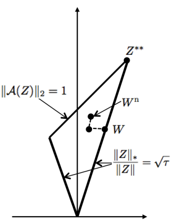
   Figure 1: Illustration of the proof for $\rho>1$.

   Actually we will show that $\rho>1$. If $\|Z^{**}\|_{*}<\sqrt{\tau}\|Z^{**}\|_{\mathrm{F}}$, we are done. If not (i.e., $\|Z^{**}\|_{*}=\sqrt{\tau}\|Z^{**}\|_{\mathrm{F}}$), as illustrated in Figure 1, we consider $W=\frac{\eta_{0}}{\gamma^{*}}Z^{**}$, which satisfies

   $$\|\mathcal{A}(W)\|_{2}=\frac{\eta_{0}}{\gamma^{*}}<1,$$ (102)

   $$\|W\|_{\mathrm{F}}=\eta_{0},\text{\ and \ }$$ (103)

   $$\|W\|_{*}=\sqrt{\tau}\eta_{0}.$$ (104)

   Suppose $\boldsymbol{\sigma}$ is the singular value vector of $W$. To get $W^{\mathrm{n}}$ as shown in Figure 1, pick the smallest non-zero singular value, and scale it by a small positive constant $\kappa$ less than $1$. Because $\tau>1$, $\boldsymbol{\sigma}$ has more than one non-zero components, elementary mathematics then show that this first scaling will decrease the ratio $\|\boldsymbol{\sigma}\|_{1}/\|\boldsymbol{\sigma}\|_{2}$. We then scale the entire vector $\boldsymbol{\sigma}$ so that its $\ell_{2}$ norm restores to its original value. This latter process of course does not change the ratio $\|\boldsymbol{\sigma}\|_{1}/\|\boldsymbol{\sigma}\|_{2}$.

   If the scaling constant $\kappa$ is close enough to $1$, $\|\mathcal{A}(W^{\mathrm{n}})\|_{2}$ will remain less than 1 due to continuity. But the good news is that the ratio $\|{\boldsymbol{\sigma}}\|_{1}/\|\boldsymbol{\sigma}\|_{2}=\|W^{\mathrm{n}}\|_{*}/\|W^{\mathrm{n}}\|_{\mathrm{F}}$ decreases, and hence $\rho\geq\frac{\sqrt{\tau}\|{W}^{\mathrm{n}}\|_{\mathrm{F}}}{\|{W}^{\mathrm{n}}\|_{*}}$ becomes greater than 1.

   Now we proceed to obtain a contradiction that $f_{\tau}(\eta^{*})>\eta^{*}$. If $\|Z^{\mathrm{c}}\|_{*}\leq\sqrt{\tau}\cdot\eta^{*}$, then it is a feasible point of

   $$\max_{Z}\|Z\|_{\mathrm{F}}$$ (105)

   $$\text{\ s.t. \ }\|\mathcal{A}(Z)\|_{2}\leq 1,\|Z\|_{*}\leq\sqrt{\tau}\cdot\eta^{*}.$$

   As a consequence, $f_{\tau}(\eta^{*})\geq\|Z^{\mathrm{c}}\|_{\mathrm{F}}\geq\eta_{0}>\eta^{*}$, contradicting $\eta^{*}$ is a fixed point and we are done. If this is not the case, i.e., $\|Z^{\mathrm{c}}\|_{*}>\sqrt{\tau}\cdot\eta^{*}$, we define a new point

   $$Z^{\mathrm{n}}=\tau Z^{\mathrm{c}}$$ (106)

   with

   $$\tau=\frac{\sqrt{\tau}\cdot\eta^{*}}{\|Z^{\mathrm{c}}\|_{*}}<1.$$ (107)

   Note that $Z^{\mathrm{n}}$ is a feasible point of the optimization problem defining $f_{\tau}(\eta^{*})$ since

   $$\|\mathcal{A}(Z^{\mathrm{n}})\|_{2}=\tau\|\mathcal{A}(Z^{\mathrm{c}})\|_{2}<1,$$ (108)

   $$\|Z^{\mathrm{n}}\|_{*}=\tau\|Z^{\mathrm{c}}\|_{*}=\sqrt{\tau}\cdot\eta^{*}.$$ (109)

   Furthermore, we have

   $$\|Z^{\mathrm{n}}\|_{\mathrm{F}}=\tau\|Z^{\mathrm{c}}\|_{\mathrm{F}}=\rho\eta^{*}.$$ (110)

   As a consequence, we obtain a contradiction

   $$f_{\tau}(\eta^{*}) \geq \rho\eta^{*}>\eta^{*}.$$ (111)

   

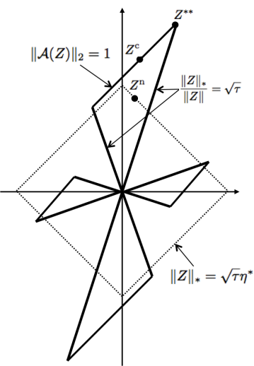
   Figure 2: Illustration of the proof for $f_{\tau}(\eta^{*})\geq\rho\eta^{*}$.

   Therefore, for the fixed point $\eta^{*}$, we have $\eta^{*}=\gamma^{*}=1/\rho_{\tau}(\mathcal{A})$.

7. This property simply follows from the continuity, the uniqueness, and property 4).

8. We use contradiction to show the existence of $\rho_{1}(\epsilon)$ in 8). In view of 4), we need only to show the existence of such a $\rho_{1}(\epsilon)$ that works for $\eta_{L}\leq\eta\leq(1-\epsilon)\eta^{*}$ where $\eta_{L}=\sup\{\eta:f_{\tau}(\xi)\geq\sqrt{\tau}\xi,\forall 0<\xi\leq\eta\}$. Suppose otherwise, we then construct sequences $\{\eta^{(k)}\}_{k=1}^{\infty}\subset[\eta_{L},(1-\epsilon)\eta^{*}]$ and $\{\rho_{1}^{(k)}\}_{k=1}^{\infty}\subset(1,\infty)$ with

   $$\lim_{k\rightarrow\infty}\rho_{1}^{(k)}=1,$$

   $$f_{\tau}(\eta^{(k)})\leq\rho^{(k)}\eta^{(k)}.$$ (112)

   Due to the compactness of $[\eta_{L},(1-\epsilon)\eta^{*}]$, there must exist a subsequence $\{\eta^{(k_{l})}\}_{l=1}^{\infty}$ of $\{\eta^{(k)}\}$ such that $\lim_{l\rightarrow\infty}\eta^{(k_{l})}=\eta_{\mathrm{lim}}$ for some $\eta_{\mathrm{lim}}\in[\eta_{L},(1-\epsilon)\eta^{*}]$. As a consequence of the continuity of $f_{\tau}(\eta)$, we have

   $$f_{\tau}(\eta_{\mathrm{lim}}) = \lim_{l\rightarrow\infty}f_{\tau}(\eta^{(k_{l})})$$ (113)

   $$\leq \lim_{l\rightarrow\infty}\rho_{1}^{(k_{l})}\eta^{(k_{l})}=\eta_{\mathrm{lim}}.$$

   Again due to the continuity of $f_{\tau}(\eta)$ and the fact that $f_{\tau}(\eta)>\eta$ for $\eta<\eta_{L}$, there exists $\eta_{c}\in[\eta_{L},\eta_{\mathrm{lim}}]$ such that

   $$f_{\tau}(\eta_{c}) = \eta_{c},$$ (114)

   contradicting the uniqueness of the fixed point for $f_{\tau}(\eta)$. The existence of $\rho_{2}(\epsilon)$ can be proved in a similar manner.

∎

Appendix D Proof of Proposition 2

In this appendix, we provide a proof of Proposition 2. For any $r$ such that the set $V\left(r\right)=\left\{X\in\mathbb{R}^{n_{1}\times n_{2}}:\left\|\Sigma_{1}^{1/2}X\Sigma_{2}^{1/2}\right\|_{F}=1,\left\|X\right\|_{\ast}\leq r\right\}$ is non-empty, define a random variable

$$M\left(r,\mathcal{A}_{\Sigma_{1},\Sigma_{2}}\right):=1-\inf_{X\in V\left(r\right)}\left\|\mathcal{A}_{\Sigma_{1},\Sigma_{2}}\left(X\right)\right\|_{2}$$ (115)

$$= \sup_{X\in V\left(r\right)}\left\{1-\left\|\mathcal{A}_{\Sigma_{1},\Sigma_{2}}\left(X\right)\right\|_{2}\right\}$$

We first show that

$$\mathbb{E}M\left(r,\mathcal{A}_{\Sigma_{1},\Sigma_{2}}\right)$$

$$\leq\frac{1}{4}+\frac{\sqrt{\operatorname*{trace}\left(\Sigma_{1}\right)}+\sqrt{\operatorname*{trace}\left(\Sigma_{2}\right)}}{\sqrt{m}}r.$$ (116)

To this end, we define two Gaussian processes indexed by $\boldsymbol{u}\in S^{m-1},X\in V\left(r\right)$

$$Y_{\boldsymbol{u},X} = \left\langle\boldsymbol{u},\mathcal{A}_{\Sigma_{1},\Sigma_{2}}\left(X\right)\right\rangle$$ (117)

$$= \sum_{k,i,j}u_{k}G^{k}_{ij}\left(\Sigma_{1}^{1/2}X\Sigma_{2}^{1/2}\right)_{ij},$$

$$Z_{\boldsymbol{u},X} = \left\langle\boldsymbol{u},\boldsymbol{g}\right\rangle+\left\langle\Sigma_{1}^{1/2}X\Sigma_{2}^{1/2},G\right\rangle,$$ (118)

where $S^{m-1}$ is the unit sphere in $\mathbb{R}^{m}$, and $g_{k},G_{ij},G_{ij}^{k}$ are i.i.d. $\mathcal{N}\left(0,1/m\right)$ random variables. Observe that

$$\sup_{X\in V\left(r\right)}\inf_{\boldsymbol{u}\in S^{m-1}}Y_{\boldsymbol{u},X}=-\inf_{X\in V\left(r\right)}\sup_{\boldsymbol{u}\in S^{m-1}}Y_{\boldsymbol{u},X}$$ (119)

$$= -\inf_{X\in V\left(r\right)}\left\|\mathcal{A}_{\Sigma_{1},\Sigma_{2}}\left(X\right)\right\|_{2}.$$

We apply Gordon’s comparision theorem [25, Chapter 3.1] which states that if

$$\mathbb{E}\left(Y_{\boldsymbol{u},X}-Y_{\boldsymbol{u}^{\prime},X^{\prime}}\right)^{2}\leq\mathbb{E}\left(Z_{\boldsymbol{u},X}-Z_{\boldsymbol{u}^{\prime},X^{\prime}}\right)^{2},$$ (120)

for all $\left(\boldsymbol{u},X\right)$, $\left(\boldsymbol{u}^{\prime},X^{\prime}\right)\operatorname*{in}S^{m-1}\times V\left(r\right)$ and the inequality becomes equality when $X=X^{\prime}$, then

$$\mathbb{E}\sup_{X\in V\left(r\right)}\inf_{\boldsymbol{u}\in S^{m-1}}Y_{\boldsymbol{u},X}\leq\mathbb{E}\sup_{X\in V\left(r\right)}\inf_{\boldsymbol{u}\in S^{m-1}}Z_{\boldsymbol{u},X}.$$ (121)

Elementary calculations show that

$$\mathbb{E}\left(Y_{\boldsymbol{u},X}-Y_{\boldsymbol{u}^{\prime},X^{\prime}}\right)^{2}$$ (122)

$$= \frac{1}{m}\sum_{k,i,j}\left(u_{k}\left(\Sigma_{1}^{1/2}X\Sigma_{2}^{1/2}\right)_{ij}-u_{k}^{\prime}\left(\Sigma_{1}^{1/2}X^{\prime}\Sigma_{2}^{1/2}\right)_{ij}\right)^{2}$$

$$\leq \frac{1}{m}\sum_{k}\left(u_{k}-u_{k}^{\prime}\right)^{2}$$

$$+\frac{1}{m}\sum_{i,j}\left(\left(\Sigma_{1}^{1/2}X\Sigma_{2}^{1/2}\right)_{ij}-\left(\Sigma_{1}^{1/2}X^{\prime}\Sigma_{2}^{1/2}\right)_{ij}\right)^{2}$$

$$= \mathbb{E}\left(Z_{\boldsymbol{u},X}-Z_{\boldsymbol{u}^{\prime},X^{\prime}}\right)^{2}$$

and

$$\mathbb{E}\left(Y_{\boldsymbol{u},X}-Y_{\boldsymbol{u}^{\prime},X}\right)^{2} = \mathbb{E}\left(Z_{\boldsymbol{u},X}-Z_{\boldsymbol{u}^{\prime},X}\right)^{2}$$ (123)

$$= \frac{1}{m}\sum_{k}\left(u_{k}-u_{k}^{\prime}\right)^{2}.$$

As a consequence, we upper bound the expectation of $M\left(r,\mathcal{A}_{\Sigma_{1},\Sigma_{2}}\right)$ as follows:

$$\mathbb{E}M\left(r,\mathcal{A}_{\Sigma_{1},\Sigma_{2}}\right)$$

$$=1+\mathbb{E}\sup_{X\in V\left(r\right)}\inf_{\boldsymbol{u}\in S^{m-1}}Y_{\boldsymbol{u},X}$$

$$\leq 1+\mathbb{E}\sup_{X\in V\left(r\right)}\inf_{\boldsymbol{u}\in S^{m-1}}Z_{\boldsymbol{u},X}$$

$$\leq 1-\mathbb{E}\left\|\boldsymbol{g}\right\|_{2}+\mathbb{E}\sup_{X\in V\left(r\right)}\left|\left\langle\Sigma_{1}^{1/2}X\Sigma_{2}^{1/2},G\right\rangle\right|.$$ (124)

For $\mathbb{E}\left\|\boldsymbol{g}\right\|_{2}$, we use a simple lower bound $\mathbb{E}\left\|\boldsymbol{g}\right\|_{2}\geq\frac{3}{4}\sqrt{\frac{m}{m}}=\frac{3}{4}$ [27]. For the last term in (124), by the definition of $V\left(r\right)$, we have

$$\mathbb{E}\sup_{X\in V\left(r\right)}\left|\left\langle\Sigma_{1}^{1/2}X\Sigma_{2}^{1/2},G\right\rangle\right|$$ (125)

$$= \mathbb{E}\sup_{X\in V\left(r\right)}\left|\left\langle X,\Sigma_{1}^{1/2}G\Sigma_{2}^{1/2}\right\rangle\right|$$

$$\leq \mathbb{E}\left\|X\right\|_{\ast}\left\|\Sigma_{1}^{1/2}G\Sigma_{2}^{1/2}\right\|$$

$$\leq r\mathbb{E}\left\|\Sigma_{1}^{1/2}G\Sigma_{2}^{1/2}\right\|.$$

The problem then boils down to estimating $\mathbb{E}\left\|\Sigma_{1}^{1/2}G\Sigma_{2}^{1/2}\right\|$, which is achieved by applying Slepian’s comparison theorem [25, Chapter 3.1] to the following two Gaussian processes indexed by $\boldsymbol{u}\in S^{n_{1}-1},\boldsymbol{v}\in S^{n_{2}-1}$:

$$Y_{\boldsymbol{u},\boldsymbol{v}} = \boldsymbol{u}^{T}\Sigma_{1}^{1/2}G\Sigma_{2}^{1/2}\boldsymbol{v},$$ (126)

$$Z_{\boldsymbol{u},\boldsymbol{v}} = \boldsymbol{u}^{T}\Sigma_{1}^{1/2}\boldsymbol{g}+\boldsymbol{v}^{T}\Sigma_{2}^{1/2}\boldsymbol{h},$$ (127)

where $\boldsymbol{g}\sim\mathcal{N}\left(0,\frac{1}{m}I_{n_{1}}\right)$ and $\boldsymbol{h}\sim\mathcal{N}\left(0,\frac{1}{m}I_{n_{2}}\right)$. It is easy to verify that the variance condition for Slepian’s comparison theorem holds:

$$\mathbb{E}\left(Y_{\boldsymbol{u},\boldsymbol{v}}-Y_{\boldsymbol{u}^{\prime},\boldsymbol{v}^{\prime}}\right)^{2}\leq\mathbb{E}\left(Z_{\boldsymbol{u},\boldsymbol{v}}-Z_{\boldsymbol{u}^{\prime},\boldsymbol{v}^{\prime}}\right)^{2}.$$ (128)

Slepian’s inequality $\mathbb{E}\sup_{\boldsymbol{u},\boldsymbol{v}}Y_{\boldsymbol{u},\boldsymbol{v}}\leq\mathbb{E}\sup_{\boldsymbol{u},\boldsymbol{v}}Z_{\boldsymbol{u},\boldsymbol{v}}$ and Jensen’s inequality then imply

$$\mathbb{E}\left\|\Sigma_{1}^{1/2}G\Sigma_{2}^{1/2}\right\|$$ (129)

$$\leq \mathbb{E}\left\|\Sigma_{1}^{1/2}\boldsymbol{g}\right\|_{2}+\mathbb{E}\left\|\Sigma_{2}^{1/2}\boldsymbol{h}\right\|_{2}$$

$$\leq \sqrt{\mathbb{E}\left\|\Sigma_{1}^{1/2}\boldsymbol{g}\right\|_{2}^{2}}+\sqrt{\mathbb{E}\left\|\Sigma_{2}^{1/2}\boldsymbol{h}\right\|_{2}^{2}}$$

$$= \frac{1}{\sqrt{m}}\left(\sqrt{\operatorname*{trace}\left(\Sigma_{1}\right)}+\sqrt{\operatorname*{trace}\left(\Sigma_{2}\right)}\right).$$

Plugging back into (124) yields

$$\mathbb{E}M\left(r,\mathcal{A}_{\Sigma_{1},\Sigma_{2}}\right)$$

$$\leq\frac{1}{4}+\frac{\sqrt{\operatorname*{trace}\left(\Sigma_{1}\right)}+\sqrt{\operatorname*{trace}\left(\Sigma_{2}\right)}}{\sqrt{m}}r.$$ (130)

We next obtain a high probability result using concentration of measure in Gauss space for Lipschitz functions. Denote $\boldsymbol{e}_{k}$ as the $k$th canonical basis vector. The following manipulation of

$$h\left(G^{1},\cdots,G^{m}\right)$$

$$:=\sup_{X\in V\left(r\right)}\left(1-\left\|\sum_{k}\left\langle G^{k},\Sigma_{1}^{1/2}X\Sigma_{2}^{1/2}\right\rangle\boldsymbol{e}_{k}\right\|_{2}\right)$$

$$=M\left(r,\mathcal{A}_{\Sigma_{1},\Sigma_{2}}\right)$$ (131)

as a function of $\left\{G^{1},\cdots,G^{m}\right\}$:

$$h\left(G^{1},\cdots,G^{m}\right)$$ (132)

$$\leq 1+\sup_{X\in V\left(r\right)}-\left\|\sum_{k}\left\langle G^{\prime k},\Sigma_{1}^{1/2}X\Sigma_{2}^{1/2}\right\rangle\boldsymbol{e}_{k}\right\|_{2}$$

$$+\sup_{X\in V\left(r\right)}\left\|\sum_{k}\left\langle G^{k}-G^{\prime k},\Sigma_{1}^{1/2}X\Sigma_{2}^{1/2}\right\rangle\boldsymbol{e}_{k}\right\|_{2}$$

$$\leq h\left(G^{\prime 1},\cdots,G^{\prime m}\right)+\sqrt{\sum_{k}\left\|G^{k}-G^{\prime k}\right\|_{F}^{2}}$$

shows that the Liptchitz constant of $h\left(G^{1},\cdots,G^{m}\right)$ is 1. Here we have used the triangle inequality for the first inequality,  Cauchy-Schwarz inequality and $\Sigma_{1}^{1/2}X\Sigma_{2}=1$ on $V\left(r\right)$ for the last inequality. By concentration of measure in Gauss space [36], we obtain

$$\mathbb{P}\left\{\left|M\left(r,\mathcal{A}_{\Sigma_{1},\Sigma_{2}}\right)-\mathbb{E}M\left(r,\mathcal{A}_{\Sigma_{1},\Sigma_{2}}\right)\right|\geq t\left(r\right)/2\right\}$$ (133)

$$\leq 2\exp\left(-mt^{2}\left(r\right)/8\right)$$

where $t\left(r\right):=\frac{1}{4}+\frac{\sqrt{\operatorname*{trace}\left(\Sigma_{1}\right)}+\sqrt{\operatorname*{trace}\left(\Sigma_{2}\right)}}{\sqrt{m}}r$, implying

$$\mathbb{P}\left\{M\left(r,\mathcal{A}_{\Sigma_{1},\Sigma_{2}}\right)\geq\frac{3t\left(r\right)}{2}\right\}$$ (134)

$$\leq 2\exp\left(-mt^{2}\left(r\right)/8\right).$$

To complete the proof, we need the following lemma whose proof is based on a peeling argument:

Lemma 3 (Lemma 3 of [27])

Consider a random objective function $f\left(\boldsymbol{v};\boldsymbol{u}\right)$ with ${\boldsymbol{u}}$ the underlying random variable and $\boldsymbol{v}\in\mathbb{R}^{p}$ the variable to be optimized with. Suppose that $g:\mathbb{R}^{p}\rightarrow\mathbb{R}_{+}$ specifies an increasing constraint function, namely, $\left\{\boldsymbol{v}:g\left(\boldsymbol{v}\right)\leq r\right\}\subseteq\left\{\boldsymbol{v}:g\left(\boldsymbol{v}\right)\leq r^{\prime}\right\}$ for $r\leq r^{\prime}$, $\Omega$ is a non-empty constraint set, and

$$E=\left\{\boldsymbol{u}:\exists\boldsymbol{v}\in\Omega\operatorname*{such}\operatorname*{that}f\left(\boldsymbol{v};\boldsymbol{u}\right)\geq 2q\left(g\left(\boldsymbol{v}\right)\right)\right\},$$

where $q:\mathbb{R}\rightarrow\mathbb{R}$ is non-negative and strictly increasing with $q\left(r\right)\geq\mu$ for all $r\geq 0$. Further assume that there exists constant $d>0$ (which may depend on some other parameters) such that

$$\mathbb{P}\left\{\boldsymbol{u}:\sup_{\boldsymbol{v}\in\Omega,g\left(\boldsymbol{v}\right)\leq r}f\left(\boldsymbol{v};\boldsymbol{u}\right)\geq q\left(r\right)\right\}$$ (135)

$$\leq 2\exp\left(-dq^{2}\left(r\right)\right).$$

Then we have

$$\mathbb{P}\left\{E\right\} \leq \frac{2\exp\left(-4d\mu^{2}\right)}{1-\exp\left(-4d\mu^{2}\right)}.$$ (136)

We apply Lemma 3 to the objective function $f\left(X;\mathcal{A}_{\Sigma_{1},\Sigma_{2}}\right)=1-\left\|\mathcal{A}_{\Sigma_{1},\Sigma_{2}}\left(X\right)\right\|_{2}$, the constraint function $g\left(X\right)=\left\|X\right\|_{\ast}$, the constraint set $\Omega=\left\{X:\left\|\Sigma_{1}^{1/2}X\Sigma_{2}^{1/2}\right\|_{F}=1\right\}$, $q\left(r\right)=\frac{3}{2}t\left(r\right)=\frac{3}{8}+\frac{3}{2}\frac{\sqrt{\operatorname*{trace}\left(\Sigma_{1}\right)}+\sqrt{\operatorname*{trace}\left(\Sigma_{2}\right)}}{\sqrt{m}}r$, and $\mu=3/8$. Since

$$\mathbb{P}\left\{\sup_{g\left(X\right)\leq r,X\in\Omega}f\left(X;\mathcal{A}_{\Sigma_{1},\Sigma_{2}}\right)\geq q\left(r\right)\right\}$$ (137)

$$\leq 2\exp\left(-cmq^{2}\left(r\right)\right),$$

Lemma 3 implies that for properly chosen constant $c>0$ the event

$$E=\{\exists X\in\Omega\text{\ such that\ }1-\left\|\mathcal{A}_{\Sigma_{1},\Sigma_{2}}(X)\right\|_{2}$$

$$\geq\frac{3}{4}+3\frac{\sqrt{\operatorname*{trace}\left(\Sigma_{1}\right)}+\sqrt{\operatorname*{trace}\left(\Sigma_{2}\right)}}{\sqrt{m}}\left\|X\right\|_{\ast}\}$$ (138)

has probability

$$\mathbb{P}\left\{E\right\} \leq 2\exp\left(-cm\right).$$ (139)

So with probability at least $1-2\exp\left(-cm\right)$ we have

$$\left\|\mathcal{A}_{\Sigma_{1},\Sigma_{2}}\left(X\right)\right\|_{2}$$

$$\geq\frac{1}{4}\left\|\Sigma_{1}^{1/2}X\Sigma_{2}^{1/2}\right\|_{F}$$

$$-3\frac{\sqrt{\operatorname*{trace}\left(\Sigma_{1}\right)}+\sqrt{\operatorname*{trace}\left(\Sigma_{2}\right)}}{\sqrt{m}}\left\|X\right\|_{\ast}.$$ (140)

Gongguo Tang (S’09–M’11) received the B.Sc. degree in mathematics from the Shandong University, China, in 2003, and the M.Sc. degree in systems science from Chinese Academy of Sciences, in 2006, and the Ph.D. degree in electrical and systems engineering from Washington University in St. Louis, St. Louis, MO, in 2011. He is currently a Postdoctoral Research Associate at the Department of Electrical and Computer Engineering, University of Wisconsin-Madison. His research interests are in the area of signal processing, convex optimization, statistics, and their applications.

Arye Nehorai (S’80–M’83–SM’90–F’94) is the Eugene and Martha Lohman Professor and Chair of the Preston M. Green Department of Electrical and Systems Engineering (ESE) at Washington University in St. Louis (WUSTL). He serves as the Director of the Center for Sensor Signal and Information Processing at WUSTL. Earlier, he was a faculty member at Yale University and the University of Illinois at Chicago. He received the B.Sc. and M.Sc. degrees from the Technion, Israel and the Ph.D. from Stanford University, California. Dr. Nehorai served as Editor-in-Chief of IEEE Transactions on Signal Processing from 2000 to 2002. From 2003 to 2005 he was the Vice President of the IEEE Signal Processing Society (SPS), the Chair of the Publications Board, and a member of the Executive Committee of this Society. He was the founding editor of the special columns on Leadership Reflections in IEEE Signal Processing Magazine from 2003 to 2006. He has been a Fellow of the IEEE since 1994 and of the Royal Statistical Society since 1996.

References

- [1] E. J. Candès and T. Tao, “Near-optimal signal recovery from random projections: Universal encoding strategies?,” IEEE Trans. Inf. Theory, vol. 52, no. 12, pp. 5406–5425, dec 2006.
- [2] D. L. Donoho, “Compressed sensing,” IEEE Trans. Inf. Theory, vol. 52, no. 4, pp. 1289–1306, apr 2006.
- [3] B. Recht, M. Fazel, and P. A. Parrilo, “Guaranteed minimum-rank solutions of linear matrix equations via nuclear norm minimization,” SIAM Review, vol. 52, no. 3, pp. 471–501, 2010.
- [4] M. Fazel, Matrix Rank Minimization with Applications, Ph.D. thesis, Stanford University, 2002.
- [5] E. J. Candès and Y. Plan, “Tight oracle inequalities for low-rank matrix recovery from a minimal number of noisy random measurements,” IEEE Trans. Inf. Theory, vol. 57, no. 4, pp. 2342–2359, apr 2011.
- [6] J. B. Tenenbaum, V. de Silva, and J. C. Langford, “A global geometric framework for nonlinear dimensionality reduction,” Science, vol. 290, no. 5500, dec 2000.
- [7] S. T. Roweis and L. K. Saul, “Nonlinear dimensionality reduction by locally linear embedding,” Science, pp. 2323–2326, dec 2000.
- [8] L. El Ghaoui and P. Gahinet, “Rank minimization under LMI constraints: A framework for output feedback problems,” in European Control Conf. Groningen, Netherland, Jun 1993.
- [9] M. Fazel, H. Hindi, and S. Boyd, “A rank minimization heuristic with application to minimum order system approximation,” in Proc. American Control Conf., vol. 6, pp. 4734–4739. 2001.
- [10] E. J. Candès and B. Recht, “Exact matrix completion via convex optimization,” Found. Comput. Math., vol. 9, no. 6, pp. 717–772, 2009.
- [11] E. J. Candès and Y. Plan, “Matrix completion with noise,” Proc. of the IEEE, vol. 98, no. 6, pp. 925–936, jun 2010.
- [12] D. Gross, Y. Liu, S. T. Flammia, S. Becker, and J. Eisert, “Quantum state tomography via compressed sensing,” Phys. Rev. Lett., vol. 105, no. 15, pp. 150401–150404, oct 2010.
- [13] R. Basri and D. W. Jacobs, “Lambertian reflectance and linear subspaces,” IEEE Trans. Pattern Anal. Mach. Intell., vol. 25, no. 2, pp. 218 – 233, feb 2003.
- [14] E. J. Candès, X. Li, Y. Ma, and J. Wright, “Robust principal component analysis?,” J. ACM, vol. 58, no. 3, pp. 1–37, jun 2011.
- [15] N. Linial, E. London, and Y. Rabinovich, “The geometry of graphs and some of its algorithmic applications,” Combinatorica, vol. 15, pp. 215–245, 1995.
- [16] A. K. Gupta and D. K. Nagar, Matrix Variate Distributions, Chapman & Hall/CRC, Boca Raton, FL, 1999.
- [17] S. Ma, D. Goldfarb, and L. Chen, “Fixed point and Bregman iterative methods for matrix rank minimization,” Mathematical Programming, vol. 120, no. 2, pp. 1–33, 2009.
- [18] P. Bickel, Y. Ritov, and A. Tsybakov, “Simultaneous analysis of Lasso and Dantzig selector,” Ann. Statist., vol. 37, no. 4, pp. 1705–1732, 2009.
- [19] N. Meinshausen and B. Yu, “Lasso-type recovery of sparse representations for high-dimensional data,” Ann. Statist., vol. 37, pp. 246–270, 2009.
- [20] B. Recht, W. Xu, and B. Hassibi, “Null space conditions and thresholds for rank minimization,” Mathematical Programming, vol. 127, no. 1, pp. 175–202, 2011.
- [21] K. J. B or oczky and R. Schneider, “Mean width of circumscribed random polytopes,” Canadian Math. Bull., vol. 53, pp. 614–628, 2010.
- [22] D. Stroock, Probability theory: An analytic view, Cambridge University Press, 1993.
- [23] K. Davidson and S. Szarek, “Local operator theory, random matrices and banach spaces,” in Handbook of the Geometry of Banach Spaces, W. B. Johnson and J. Lindenstrauss, Eds., vol. 1, pp. 317–366. North Holland, New York, NY, 2001.
- [24] R. Vershynin, Lecture notes on non-asymptotic random matrix theory, 2007.
- [25] M. Ledoux and M. Talagrand, Probability in Banach spaces: Isoperimetry and processes, Springer-Verlag, New York, 1991.
- [26] S. Mendelson, A. Pajor, and N. Tomczak-Jaegermann, “Reconstruction and subgaussian operators in asymptotic geometric analysis,” Geometric And Functional Analysis, vol. 14, no. 7, pp. 1248–1282, nov 2007.
- [27] G. Raskutti, M. J. Wainwright, and B. Yu, “Restricted eigenvalue properties for correlated Gaussian designs,” Journal of Machine Learning Research, vol. 11, pp. 2241– 2259, 2010.
- [28] M. Rudelson and S. Zhou, “Reconstruction from anisotropic random measurements,” ArXiv e-prints, June 2011.
- [29] S. Negahban and M. J. Wainwright, “Estimation of (near) low-rank matrices with noise and high-dimensional scaling,” ArXiv e-prints, Dec. 2009.
- [30] G. Tang and A. Nehorai, “Verifiable and computable performance analysis of sparsity recovery,” ArXiv e-prints, Feb. 2011.
- [31] G. Tang and A. Nehorai, “Fixed point theory and semidefinite programming for computable performance analysis of block-sparsity recovery,” ArXiv e-prints, Oct. 2011.
- [32] E. J. Candès, “The restricted isometry property and its implications for compressed sensing,” Compte Rendus de l’Academie des Sciences, Paris, Serie I, vol. 346, pp. 589–592, 2008.
- [33] G. Tang and A. Nehorai, “Performance analysis of sparse recovery based on constrained minimal singular values,” IEEE Trans. Signal Process., vol. 59, no. 12, pp. 5734–5745, Dec. 2011
- [34] C. Berge, Topological Spaces, Dover Publications, Mineola, NY, reprinted 1997 in paperback.
- [35] A. Tarski, “A lattice-theoretical fix point theorem and its applications,” Pacific Journal of Mathematics, vol. 5, pp. 285–309, 1955.
- [36] P. Massart, Concentration inequalities and model selection, Springer, New York, 2003.