A bipolar outflow from the massive protostellar core W51e2-E

Abstract

We present high resolution images of the bipolar outflow from W51e2, which are produced from the Submillimeter Array archival data observed for CO(3-2) and HCN(4-3) lines with angular resolutions of $0.^{\prime\prime}8\times 0.^{\prime\prime}6$ and $0.^{\prime\prime}3\times 0.^{\prime\prime}2$, respectively. The images show that the powerful outflow originates from the protostellar core W51e2-E rather than from the ultracompact H_II region W51e2-W. The kinematic timescale of the outflow from W51e2-E is about 1000 yr, younger than the age ($\sim$5000 yr) of the ultracompact H_II region W51e2-W. A large mass-loss rate of $\sim 1\times 10^{-3}$M_☉ yr^-1 and a high mechanical power of 120 $L_{\sun}$ are inferred, suggesting that an O star or a cluster of B stars are forming in W51e2-E. The observed outflow activity along with the inferred large accretion rate indicates that at present W51e2-E is in a rapid phase of star formation.

1. INTRODUCTION

Molecular outflows from protostellar cores provide a critical means to transport angular momentum from the accretion disk into the surrounding environment. The molecular outflows and infalls vigorously affect the turbulence and dissipation of molecular gas in molecular cores, playing an important role in the formation and evolution of massive stars. Observations of outflows can reveal the history of mass-loss processes in a protostellar system. In particular, high angular resolution observations of outflows can precisely determine the origin of an outflow and separate the outflow from the infall in a protostellar core. Nearly half of the observed molecular outflows are driven by massive protostars ($L_{\rm bol}>10^{3}L_{\sun}$) and have a typical dynamical age of $\sim 10^{4}$ yr and a mass outflow rate of $\sim 10^{-3}$ M_☉ yr^-1 (e.g. Churchwell, 2002).

W51e2, located at a distance of 5.1 kpc (Xu et al., 2009), is a prototypical core for massive star formation. The molecular core is associated with an ultracompact H_II region (e.g. Scott, 1978; Gaume et al., 1993) and a possible inflow (e.g. Ho & Young, 1996; Zhang et al., 1998; Sollins et al., 2004; Shi et al., 2010). With high-resolution observations using the Submillimeter Array (SMA) at the wavelengths of 0.85 and 1.3 mm, W51e2 was resolved into four sub-cores (Shi et al., 2010) including the ultracompact H_II region (W51e2-W) and a massive protostellar core (W51e2-E). From the analysis of the HCN(4-3) absorption line, Shi et al. (2010) showed that the bright dust core, W51e2-E, $0.^{\prime\prime}9$ east of W51e2-W, dominates the mass accretion in the region. A bipolar outflow has been detected in the W51e2 region (Keto & Klaassen, 2008) based on the SMA observations of CO(2-1) line with an angular resolution of $\sim 1\arcsec$. However, the resolution of the CO(2-1) observation was not adequate to determine the origin of the molecular outflow.

High angular resolution observations are imperative to identify the origin of the molecular outflow. In this Letter, we present high-resolution images of the bipolar outflow using the SMA data of the HCN(4-3) and CO(3-2) lines observed at 0.85 and 0.87 mm with angular resolutions of $0.^{\prime\prime}3\times 0.^{\prime\prime}2$ and $0.^{\prime\prime}8\times 0.^{\prime\prime}6$, respectively. We determine and discuss the physical properties of W51e2-E and W51e2-W cores, and assess the roles of the outflow in the process of massive star formation in W51e2.

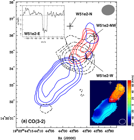
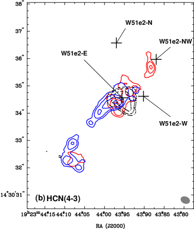
Figure 1.— (a) SMA image of W51e2 for CO(3-2) line emission at 0.87 mm, integrated from the velocity ranges of $-124$ to $-12$ km s^-1 (blue contours) and +10 to +116 km s^-1 (red contours). The integrated absorption (dashed contours) corresponds to the velocity range $-11$ to +9 km s^-1. The contours are $\pm 5\sigma\times 2^{n}$ Jy beam^-1 km s^-1 ($n=0$, 1, 2, 3, …), where $\sigma=$1.2, 1.3, and 0.63 Jy beam^-1 km s^-1 for the blue-, red-shifted emission, and absorption, respectively. The FWHM beam is $0.^{\prime\prime}79\times 0.^{\prime\prime}62$ (P.A.=$-80\arcdeg$) shown at top right. The top left inset is the CO(3-2) absorption spectrum toward W51e2-E. The bottom right inset is the intensity-weighted velocity image derived from the CO(3-2) line data (the color wedge representing the velocity range $-64$ to +76 km s^-1 relative to V_LSR=53.9 km s^-1), excluding the absorption and insignificant emission ($<3\sigma$). Crosses mark the positions of the sub-cores in W51e2 (Shi et al., 2010). (b) SMA image of W51e2 for HCN(4-3) line at 0.85 mm, integrated from the same velocity range as CO(3-2) in (a). The contours are $\pm 5\sigma\times 2^{n}$ Jy beam^-1 km s^-1 ($n=0$, 1, 2, 3, …), where $\sigma=$0.71, 0.67, and 0.31 Jy beam^-1 km s^-1 for the blue-, red-shifted emission, and absorption, respectively. The FWHM beam is $0.^{\prime\prime}33\times 0.^{\prime\prime}24$ (P.A.=$68\arcdeg$) shown at bottom right.

2. Data reduction

The interferometer data for the HCN(4-3) and CO(3-2) lines at $\nu_{0}=$ 354.505 and 345.796 GHz were acquired from the SMA archive, observed on 2007 June 18 and 2008 July 13 with the “very extended” and “extended” array configurations, respectively. The reduction for the HCN(4-3) line data was made in Miriad (Sault et al., 1995) following the reduction instructions for SMA data, which has been discussed in Shi et al. (2010). We constructed image cubes for the HCN(4-3) line with a channel width of 1 km s^-1 and an FWHM beam of $0.^{\prime\prime}33\times 0.^{\prime\prime}24$ (P.A.=68$\arcdeg$). The typical rms noise in a channel image is 0.07 Jy beam^-1.

The CO(3-2) line is included in the SMA observations at 0.87 mm for the polarization study of W51e2 that was discussed by Tang et al. (2009). The cross-polarization data were flagged before processing the data in Miriad. The data scans on 3C454.3 were used for bandpass calibration. QSO J$1751+096$ was used for calibration of the complex gains, and Uranus was used to determine the flux-density scale. The continuum level was subtracted from the line channels using UVLIN. The continuum-free line data were used for imaging with the natural weighting and a channel width of 1 km s^-1. A typical rms noise of 0.14 Jy beam^-1 and an FWHM beam of $0.^{\prime\prime}79\times 0.^{\prime\prime}62$ (P.A.=$-80\arcdeg$) were achieved for a channel image.

The shortest UV lengths in the visibility data are 30 k$\lambda$ and 54 k$\lambda$, corresponding to angular sizes of about 7$\arcsec$ and 4$\arcsec$ for the CO and HCN structure, respectively. The compact structure ($<$3″) of the outflow in both CO and HCN appears to be adequately sampled in the SMA observations. However, the total line flux density of the outflow may be underestimated due to missing short spacing. From a visibility model for the outflow source with a $uv$ coverage identical to the SMA data, we assess that $\leq$2% and $\leq$8% in the CO and HCN line flux densities may be underestimated, respectively.

3. Results

3.1. Morphologies of the bipolar outflow

Figure 1(a) shows the CO(3-2) image of W51e2 for the integrated blue-shifted ($-$124 to $-$12 km s^-1) and red-shifted (+10 to +116 km s^-1) emission and absorption ($-$11 to +9 km s^-1) with respect to the systemic velocity of $V_{\rm LSR}=$ 53.9 km s^-1 (Shi et al., 2010). The outflow velocities discussed throughout the Letter are with respect to this systemic velocity. The low velocity limits were determined by the velocities at the boundary of the absorption region. The high velocity limits correspond to the velocities at which the high-velocity wing profiles drop to the 1$\sigma$ level. The ranges of velocities for the outflow wings are also valid for the CO(2-1) and HCN(4-3) line profiles. The CO(3-2) line profiles appear to be contaminated by three narrow ($\Delta V_{\rm FWHM}\approx 6$ km s^-1) anonymous lines at the velocities of –104, –89 and +70 km s^-1. Prior to integrating the CO(3-2) line from the outflow, the line emission in the velocity ranges from –117 to –79 and from +62 to +76 km s^-1 is blanked. Thus, about 20% and 10% of the line fluxes are missing in the blue- and red-shifted outflow lobes shown in Figure 1(a), respectively.

The CO(3-2) image shows a stronger blue-shifted lobe in the southeast with a position angle of $140\arcdeg\pm 6\arcdeg$ (from north to east) and a weaker red-shifted lobe in northwest ($-40\arcdeg\pm 11\arcdeg$), which are in agreement with the outflow structure revealed in the CO(2-1) image (Keto & Klaassen, 2008). With Gaussian fitting, we determined the intrinsic sizes of $2.^{\prime\prime}3\times 0.^{\prime\prime}6$ and $1.^{\prime\prime}1\times 0.^{\prime\prime}6$ for the blue- and red-shifted lobes, respectively. Our high resolution CO(3-2) image clearly shows that the molecular bipolar outflow originates from W51e2-E (the protostellar core) rather than W51e2-W (the ultracompact H_II region). The bright emission ridge along the northeast edge of the blue-shifted lobe corresponds to a high-velocity component of the outflow, or an outflow jet (see the velocity distribution image in the lower right inset of Figure 1(a)). The weak, relatively extended emission along the southwest edge of the blue-shifted lobe may indicate a backflow of the molecular gas from the interaction between the outflows and the medium surrounding the W51e2 core. In addition, a velocity gradient is present along the major axis of the red-shifted lobe, with higher velocities near the core, indicating that the gas in the red-shifted outflow is decelerated. By averaging the intensity-weighted velocities along the bright emission ridges in both the blue- and red-shifted lobes, we infer the mean radial velocities of $\bar{V}_{\rm blue}=-34\pm 7$ and $\bar{V}_{\rm red}=+52\pm 2$ km s^-1 for the outflow lobes. The CO(3-2) spectrum toward W51e2-E also shows a large fraction of absorption to be red-shifted relative to the systemic velocity (top left inset of Figure 1(a)), suggesting the presence of infalling gas, which agrees with the results from the observations of the CO(2-1) and HCN(4-3) lines (Shi et al., 2010).

Table 1Outflow Parameters from CO(3-2) and CO(2-1) Lines.

Quantities	CO(3-2)		CO(2-1)
	Blue	Red	Blue	Red
$V$ range (km s-1)	–124 to –12	+10 to +116	–124 to –12	+10 to +116
$\bar{V}$ (km s-1)	$-34\pm 7$	$+52\pm 2$	…	…
$\Delta V$ (km s-1)a	19$\pm$5	33$\pm$8	14$\pm$2	19$\pm$4
Outflow intrinsic size $\theta_{\rm Maj}$ (″)	$2.3\pm 0.3$	$1.1\pm 0.4$	…	…
Outflow intrinsic size $\theta_{\rm Min}$ (″)	$0.6\pm 0.5$	$0.6\pm 0.6$	…	…
Outflow P.A. (°)	$140\pm 6$	$-40\pm 11$	…	…
$\int\Delta I(v){\rm d}v$ (Jy beam-1 km s-1)a	$120_{-18}^{+30}$	$80_{-12}^{+15}$	$59\pm 6$	$25\pm 3$
$\Delta I(\nu_{\rm p})$ (Jy beam-1)a	6.5$\pm$1.0	2.4$\pm$0.4	4.3$\pm$0.4	1.3$\pm$0.2
$\Delta T_{\rm L}(\nu_{\rm p})$ (K)a,b	112$\pm$17	41$\pm$7	$>100$	$>30$
$f_{\rm B}^{\rm b}$	0.6	0.6	$\leq 1$	$\leq 1$
$T_{\rm ex}$ (K)	120	65	120	65
$\tau_{\rm L}(\nu_{\rm p})$	3.9	1.3	1.9	0.7
$N_{\rm H_{2}}$ ($10^{22}$cm-2)c	6.4	1.3	…	…
$M_{\rm out}$ (M☉)	1.3	0.1	…	…
$t_{\rm out}$ (yr)d	1600/tan($i$)	500/tan($i$)	…	…
Notes:
aThe quantities at the maximum positions of the CO(3-2) flux. $\Delta V=\int\Delta I(v){\rm d}v/\Delta I(\nu_{p})$.
bThe beam filling factor ($f_{\rm B}$) is the ratio of the minor-axis size to the beam size projected on the minor axis and
$\Delta T_{\rm L}(\nu_{\rm p})=\frac{c^{2}}{2k}\nu_{\rm p}^{-2}\Delta I(\nu_{\rm p})f_{\rm B}^{-1}$.
c${N_{\rm H_{2}}=8\times 10^{17}T_{\rm ex}{\rm exp}\left(\frac{16.6}{T_{\rm ex}}\right)\left[{1-{\rm exp}(\frac{-16.6}{T_{\rm ex}})}\right]^{-1}\int\tau_{L}{\rm d}v}$ $\approx 5\times 10^{16}{\rm cm^{-2}}T_{\rm ex}^{2}{\rm exp}\left(\frac{16.6}{T_{\rm ex}}\right)\tau_{L}(\nu_{\rm p})\Delta V$ for CO(3-2)
assuming an abundance of ${\left[N_{\rm CO}\right]/\left[N_{\rm H_{2}}\right]=10^{-4}}$.
d$i$ is the angle between the major axis of outflow and line of sight.

The HCN(4-3) image in Figure 1(b) shows the high-density gas components in the bipolar outflow. At the resolution of $0.^{\prime\prime}3\times 0.^{\prime\prime}2$, the SMA image unambiguously verifies that W51e2-E is the driving source for the bipolar outflow in the region. We also noticed that the HCN emission traces the northeast edge of the blue-shifted lobe where the CO(3-2) emission shows a sharp gradient both in intensity and velocity, suggesting that the line emission of the molecular HCN is likely enhanced near the shocked or compressed regions of an outflow (Bachiller & Perez Gutierrez, 1997). In addition, at the southeastern tip of the blue-shifted outflow lobe, an “L” shape structure is detected in the HCN(4-3) emission with a double spectral feature at $\rm V\approx-14$ and +16 km s^-1, each of the spectral profiles having a line width of $\Delta V_{\rm FWHM}\sim 15$ km s^-1. The HCN line emission suggests that the gas in the region is swept up by the suspected bow shock at the tip of the outflow.

The polarization emission detected in the W51e2 region shows a “hourglass” shape in magnetic fields, which is probably related to the gas infall and disk rotation (Tang et al., 2009). Our images for the bipolar outflow in both the CO(3-2) and HCN(4-3) lines (Figures 1(a) and (b)) show that, located near the “hourglass” center, W51e2-E appears to be the energy source responsible for both the magnetic fields and the bipolar outflow. The “hourglass” structure appears to slightly extend along the major axis of the outflow, suggesting that the magnetic fields might also be tangled with the outflow motions.

3.2. Physical properties

The bipolar outflows from W51e2-E have been detected in both CO(3-2) and CO(2-1) with the SMA. In order to assess the physical conditions of the outflow gas, we re-processed the CO(2-1) data and convolved the CO(3-2) image to the same beam size as that of the CO(2-1) image ($1.^{\prime\prime}4\times 0.^{\prime\prime}7$). For both the CO(3-2) and CO(2-1) lines, the line peak ($\nu=\nu_{\rm p}$) brightness temperatures $\Delta T_{L}(\nu_{\rm p})$ of the blue- and red-shifted line profiles can be determined from the maximum positions of the CO(3-2) line fluxes in Figure 1. Then, the optical depth at the line peak can be estimated if the gas is in local thermal equilibrium (LTE) (Rohlfs & Wilson, 2004) and the cosmic microwave background (CMB) radiation is negligible,

$$\tau_{L}(\nu)=-{\rm ln}\left[1-\frac{\Delta T_{L}(\nu)}{T_{0}(\nu)}\left({\rm e}^{\frac{T_{0}(\nu)}{T_{\rm ex}}}-1\right)\right],$$ (1)

where $T_{\rm ex}$ is the excitation temperature of the transition and $T_{0}(\nu)=h\nu/k$. Thus, each of $\tau(\nu)_{(3-2)}$ and $\tau(\nu)_{(2-1)}$ can be determined independently from Equation (1) at a given $T_{\rm ex}$. On the other hand, under the assumption of LTE, the optical-depth ratio between CO(3-2) and CO(2-1) can be independently expressed as

$$\frac{\tau_{L}(\nu)_{(3-2)}}{\tau_{L}(\nu)_{(2-1)}} = \frac{(S\mu^{2})_{(3-2)}}{(S\mu^{2})_{(2-1)}}\frac{{\rm e}^{\frac{T_{0}(3-2)}{T_{\rm ex}}}-1}{{\rm e}^{\frac{T_{0}(2-1)}{T_{\rm ex}}}-1}{\rm e}^{-\frac{T_{0}(3-2)}{T_{\rm ex}}},$$ (2)

where $S$ and $\mu$ are the line strength and the permanent electric dipole moment, respectively. For the two given transitions, such as CO(3-2) and CO(2-1), the ratio of the optical depth ($\displaystyle\tau_{L(3-2)}/\tau_{L(2-1)}$) depends only on the excitation temperature $T_{\rm ex}$ (Equation (2)). By giving an initial value of $T_{\rm ex}$, the three unknown quantities ($\tau_{L(3-2)}$, $\tau_{L(2-1)}$, and $T_{\rm ex}$) can be solved with a few iterative steps from Equations (1) and (2), constrained by the measured quantities $\Delta T_{L(3-2)}$ and $\Delta T_{L(2-1)}$ for each of the blue- and red-shifted lobes.

Table 1 summarizes the results of the physical parameters determined for the molecular outflow. For the quantities directly determined from the CO images, the estimated 1$\sigma$ uncertainties are given. The excitation temperatures of 120 and 65 K are derived for the blue- and red-shifted CO outflow lobes, respectively. The optical depths of the blue-shifted CO lines are $\tau_{L(3-2)}=$3.9 and $\tau_{L(2-1)}=$ 1.9, and the red-shifted lobe are $\tau_{L(3-2)}=$1.3 and $\tau_{L(2-1)}=$ 0.7. Uncertainties of $\sim$30% in the derived values for $T_{\rm ex}$ and $\tau_{L}$ are mainly due to the uncertainties in the determination of the line flux densities. The H₂ column density (6.4$\times 10^{22}$ cm^-2) in the blue-shifted lobe appears to be a few times greater than the value derived from the red-shifted lobe ($1.3\times 10^{22}$ cm^-2). Considering the intrinsic size of the outflow, we infer that the total outflow mass is about 1.4 M_☉. From the intrinsic sizes ($\theta_{\rm Maj}$) and the intensity-weighted mean velocity ($\bar{V}$) of the outflow components, the kinematic timescale ($t_{\rm out}$) is found to be $\sim$1000 yr if the outflow inclination angle is taken as $i\sim 45$°. Therefore, the mass-loss rate and momentum rate are 1$\times 10^{-3}$ M_☉ yr^-1 and 0.04 M_☉ km s^-1 yr^-1 from W51e2-E, respectively. The mass-loss rate has the same order of magnitude as the value of the accretion rate ($>1\times 10^{-3}$ M_☉ yr^-1; Shi et al., 2010) derived from the HCN(4-3) absorption line toward W51e2-E. The momentum rate corresponds to a mechanical power of 120 $L_{\sun}$, which is at least an order of magnitude greater than that of an early type B star (e.g. Churchwell, 1999; Arce et al., 2007), suggesting that the protostellar core W51e2-E is forming an O type star or a cluster of B type stars.

4. Discussions

The current star formation activities in the W51e2 complex are shown by the powerful bipolar outflow originating from W51e2-E, in contrast to the ultracompact H_II region W51e2-W detected at 6 cm (Scott, 1978). The central region of W51e2-W ($<0.06\arcsec$), characterized by a hypercompact H_II component (see the H26$\alpha$ line emission region in Figure 2) with $T_{e}=12,000$ K, is surrounded by an expanding ionized component with a mean temperature of 4900 K (Shi et al., 2010). The mean density of $3.0\times 10^{5}$ cm^-3 and a Lyman photon rate of $3.0\times 10^{48}$ s^-1 were also derived. Using a classic model for the expansion of an H_II region (Garay & Lizano, 1999), we estimated the dynamic age of the H_II region as the time of the sound wave traveling from the initial ionization front at a radius close to the Str$\ddot{\rm o}$mgren radius ($r_{s}$; Strömgren, 1939) to the current ionization front at a radius of $r_{i}$:

$$t=\frac{4}{7}\left[\left(\frac{r_{i}}{r_{s}}\right)^{7/4}-1\right]\frac{r_{s}}{C_{\rm II}}.$$ (3)

Here $r_{i}$ can be determined from radio continuum observations of the H_II region, we adopted the size of $<2.5\arcsec$ which corresponds to $r_{i}<0.03$ pc from the result of 3.6 cm continuum observation by Mehringer (1994). We derived the Str$\ddot{\rm o}$mgren radius of 0.008 pc using the mean physical parameters inferred above. The sound speed of the ionized medium is $C_{\rm II}=\sqrt{\gamma kT_{e}/m_{p}}$, where $m_{p}$ is the mass of the proton and $k$ is the Boltzmann constant. Assuming the adiabatic index $\gamma=\frac{5}{3}$ and an average $T_{e}=4900$ K, we found $C_{\rm II}\approx 8.2$ km s^-1. Therefore, the dynamic age for the ultracompact H_II region W51e2-W is about $5000$ yr, which appears to be a few times older than the outflow from W51e2-E (see $t_{\rm out}$ in Table 1).

High-resolution observations of absorption spectra of the HCN(4-3) from W51e2-E and W51e2-W show that at present W51e2-E dominates the gas accretion from the molecular core W51e2 (see the HCN(4-3) absorption region, blue color in Figure 2). If the accretion rate is a constant of 1.3$\times 10^{-3}$ M_☉ yr^-3 (Shi et al., 2010), W51e2-E would have accreted a total of $\sim$6 M_☉ over the 5000 yr period, $<$5% of the total mass (140 M_☉; Shi et al. 2010) of the sub-core. Thus, most of the mass accumulation for W51e2-E probably occurred before the star(s) formed in the ultracompact H_II region W51e2-W. After an O8 star or a cluster of B type stars formed in W51e2-W, the overwhelming radiation pressure and strong turbulence in W51e2-W halted the accretion in the sub-core region. Therefore, W51e2-E might speed up its formation of stars since W51e2-W is no longer competing for accretion.

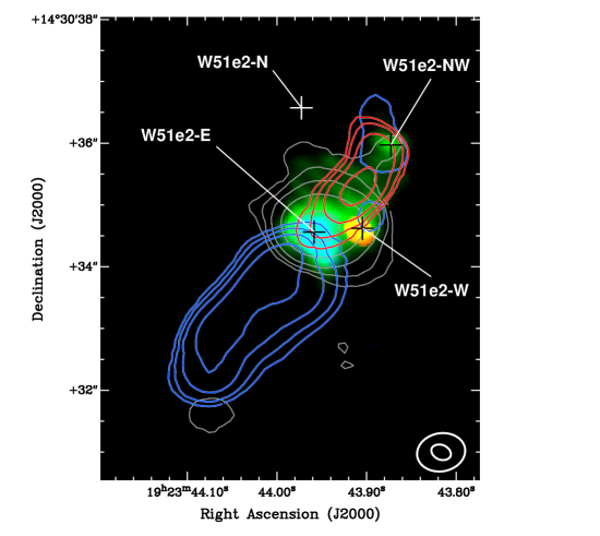
Figure 2.— RGB composition image of H26$\alpha$ emission (red), 0.85 mm continuum emission (green), and HCN(4-3) absorption (blue) observed with the SMA at a resolution of $0.^{\prime\prime}33\times 0.^{\prime\prime}24$ (P.A.=68$\arcdeg$; Shi et al., 2010) overlaid with the contour map of CO(3-2) outflow (red and blue) and absorption (grey) (Figure 1a). Crosses mark the positions of the sub-cores.

In summary, a bipolar molecular outflow in W51e2 is confirmed and the massive protostellar core W51e2-E is identified to be the origin of this powerful outflow. In comparison to the ultracompact H_II region W51e2-W, W51e2-E appears to be the dominant accretion source at present, where the active formation of massive stars takes place.

References

- Arce et al. (2007) Arce, H. G., Shepherd, D., Gueth, F., Lee, C.-F., Bachiller, R., Rosen, A., & Beuther, H. 2007, in Protostars and Planets V, ed.B.Reipurth, D.Jewitt, & K.Keil (Tucson, AZ: Univ. Arizona Press), 245
- Bachiller & Perez Gutierrez (1997) Bachiller, R. & Perez Gutierrez, M. 1997, ApJ, 487, L93
- Churchwell (1999) Churchwell, E. 1999, in NATO ASIC Proc. 540, The Origin of Stars and Planetary Systems, ed. C. J. Lada & N. D. Kylafis (Dordrecht: Kluwer), 515
- Churchwell (2002) Churchwell, E. 2002, ARA&A, 40, 27
- Garay & Lizano (1999) Garay, G. & Lizano, S. 1999, PASP, 111, 1049
- Gaume et al. (1993) Gaume, R. A., Johnston, K. J., & Wilson, T. L. 1993, ApJ, 417, 645
- Ho & Young (1996) Ho, P. T. P. & Young, L. M. 1996, ApJ, 472, 742
- Keto & Klaassen (2008) Keto, E. & Klaassen, P. 2008, ApJ, 678, L109
- Mehringer (1994) Mehringer, D. M. 1994, ApJS, 91, 713
- Rohlfs & Wilson (2004) Rohlfs, K. & Wilson, T. L. 2004, Tools of Radio Astronomy, ed. Rohlfs, K. & Wilson, T. L. (Berlin: Springer)
- Sault et al. (1995) Sault, R. J., Teuben, P. J., & Wright, M. C. H. 1995, ASP Conf. Ser. 77, Astronomical Data Analysis Software and Systems IV, ed. R. A. Shaw, H. E. Payne, & J. J. E. Hayes (San Francisco, CA: ASP), 433
- Scott (1978) Scott, P. F. 1978, MNRAS, 183, 435
- Shi et al. (2010) Shi, H., Zhao, J.-H., & Han, J. L. 2010, ApJ, 710, 843
- Sollins et al. (2004) Sollins, P. K., Zhang, Q., & Ho, P. T. P. 2004, ApJ, 606, 943
- Strömgren (1939) Strömgren, B. 1939, ApJ, 89, 526
- Tang et al. (2009) Tang, Y.-W., Ho, P. T. P., Koch, P. M., Girart, J. M., Lai, S.-P., & Rao, R. 2009, ApJ, 700, 251
- Xu et al. (2009) Xu, Y., Reid, M. J., Menten, K. M., Brunthaler, A., Zheng, X. W., & Moscadelli, L. 2009, ApJ, 693, 413
- Zhang et al. (1998) Zhang, Q., Ho, P. T. P., & Ohashi, N. 1998, ApJ, 494, 636