Model of the response function of large mass bolometric detectors

Abstract

Large mass bolometers are used in particle physics experiments to search for rare processes. By operating at low temperature, they are able to detect particle energies from few keV up to several MeV, measuring the temperature rise produced by the energy released. This study was performed on the bolometers of the CUORE experiment. The response function of these detectors is not linear in the energy range of interest, and it changes with the operating temperature. The non-linearity is found to be dominated by the thermistor and its biasing circuit, and is modeled using few measurable parameters. A method to obtain a linear response is the result of this work. It allows a great simplification of the data analysis.

I Introduction

Bolometers are detectors where the energy of particle interactions is converted into heat and measured via temperature variation. They provide an excellent energy resolution, although they are slow compared to conventional detectors. These features make them a suitable choice for experiments looking to rare processes, like neutrinoless double beta decay and dark matter interactions.

The CUORE experiment searches for neutrinoless double beta decay in ${}^{130}\mathrm{Te}$ Ardito et al. (2005), using bolometers made of $\mathrm{TeO}_{2}$ crystals whose temperature is measured by neutron transmutation doped (NTD) Germanium semiconductor thermistors Wang et al. (1990); Itoh et al. (1994). Operated at temperatures of about $10\mathrm{\,mK}$, these detectors maintain a resolution of few keV over their energy range, extending from few keV up to several MeV. In this range the response function is found to be non-linear. The conversion from signal amplitude to energy is complicated and the shape of the signal depends on the energy itself. Moreover the amplitude of the signal depends on the temperature of the detector, which cannot be kept stable by current cryostats at a level that would not perturb the resolution. Understanding the non-linearities is important to have a reliable calibration, to control the signal shape and to improve the resolution.

Electrothermal models for large mass bolometers have been already proposed JONES (1953); Alessandrello et al. (1993); McCammon (2004). Based on systems of differential equations, they describe the behavior of the detector and reproduce the shape of the signal and some features of the calibration function. However, they rely on many parameters that are difficult to measure with the necessary precision in working conditions. These models are useful to describe the response of a bolometer, but they cannot produce tools to be used on a real detector.

In this paper a model based on few parameters is proposed. It shows that the non-linearities are dominated by the thermal sensor and by the biasing circuit that is used to read it. These elements are fully measurable in working conditions, so that the model can be applied to the detector. A method to remove the non-linearities is derived. Its application in the data analysis linearizes the response function, improving the results.

II Description of the detector

A CUORE bolometer is composed of two main parts, a $\mathrm{TeO}_{2}$ crystal and a NTD-Ge thermistor. The crystal is cube-shaped, weighs 750$\mathrm{\,g}$ and its heat capacitance $C$ at the working temperature of 10$\mathrm{\,mK}$ is of order 2$\mathrm{\,nJ/K}$ Barucci et al. (2001). It is held by Teflon supports on copper frames, which are connected to the mixing chamber of a dilution refrigerator. The thermistor is glued to the crystal and the biasing wires are glued to the copper frames (see Fig. 1) .

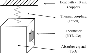
Figure 1: Sketch of a CUORE bolometer. The $\mathrm{TeO}_{2}$ crystal is held by Teflon supports, the thermistor is glued to the crystal and its wires are glued to copper frames. The supports and the thermistor wires thermally couple the crystal to the copper frames, which act as heat bath.

When an amount of energy $E$ is released in the crystal, its temperature increases by $E/C$ and then returns to equilibrium via the thermal conductance of the supports and of the thermistor. The latter acts as thermometer, converting temperature, $T$, into resistance, $R$, according to the relationship Mott (1969):

$$R(T)=R_{0}\exp\left(T_{0}/T\right)^{\gamma}$$ (1)

where $R_{0}$ and $T_{0}$ are parameters that depend on the dimensions and on the material of the thermistor. Their value is about $1.1\mathrm{\,\mathrm{\,\Omega}}$ and $3.4\mathrm{\,K}$ respectively. At 10$\mathrm{\,mK}$ the parameter $\gamma$ can be considered constant and equal to $1/2$  Efros and Shklovskii (1984); Itoh et al. (1996).

To read out the signal, the thermistor is biased with constant current, which is provided by a voltage generator, $V_{B}$, and a load resistor, $R_{L}$, in series with the thermistor. The resistance of the thermistor varies in time with the temperature, $R(t)$, and the voltage across it, $V(t)$, is the bolometer signal. The value of $R_{L}$ is chosen to be much higher than $R(t)$ so that $V(t)$ is almost proportional to $R(t)$. Since from Eq. (1) positive temperature variations induce negative resistance variations, the voltage $V_{B}$ is chosen to be negative in order to obtain positive signals. The connecting wires add in parallel to the thermistor a parasitic capacitance $c_{p}$ (see Fig. 2). The signal $V(t)$ is amplified, filtered with a 6-pole active Bessel filter and then acquired with an 18 bit DAQ system. The front end electronics, which provide the bias, the load resistors, and the amplifier, are placed outside the cryostat, at room temperature Arnaboldi et al. (2002).

Figure 2: Biasing circuit of the thermistor. A voltage generator $V_{B}$ biases the thermistor resistance $R(t)$ in series with a load resistance $R_{L}$. The bolometer signal is the voltage $V(t)$ across $R(t)$. The wires used to read $V(t)$ have a non-negligible capacitance $c_{p}$.

At 10$\mathrm{\,mK}$ the value of $R(T)$ is of order $100\mathrm{\,M\mathrm{\,\Omega}}$, $R_{L}$ is chosen as $\sim 50\mathrm{\,G\mathrm{\,\Omega}}$ and $V_{B}$ as $\sim 5$$\mathrm{\,V}$. The $c_{p}$ value depends on the length of the wires that carry the signal out of the cryostat, typically it is of order 400$\mathrm{\,pF}$. The amplifier gain, the Bessel frequency bandwidth, the duration of the acquisition window and the sampling frequency are set typically at 5000$\mathrm{\,V/V}$, 12$\mathrm{\,Hz}$, 5.008$\mathrm{\,s}$ and 125$\mathrm{\,Hz}$ respectively.

A typical signal acquired by the ADC, is shown in Fig. 3.

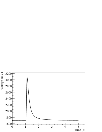
Figure 3: Pulse generated by a 2615$\mathrm{\,keV}$ $\gamma$ particle. The baseline is related to the temperature of the thermistor before the particle interaction, the amplitude carries information on the amount of energy released.

The signal was generated by a 2615$\mathrm{\,keV}$ $\gamma$ particle fully absorbed in the crystal. The baseline voltage of the pulse is related to the thermistor temperature before the particle interaction, and the amplitude is related to the energy released.

III Non-linearities of the response function

The data analyzed in this paper have been obtained by exposing the bolometer to a ²³²Th source. This source, together with an $\alpha$ line generated by ²¹⁰Po contamination of the crystal, allows the analysis of an energy range up to 5407$\mathrm{\,keV}$ (see the energy spectrum in Fig. 4).

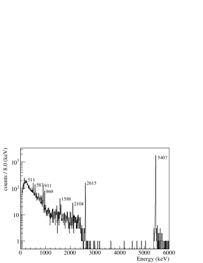
Figure 4: Energy Spectrum. The $\alpha$ line at 5407$\mathrm{\,keV}$ is generated by ²¹⁰Po contamination of the crystal, the rest of the spectrum is due to $\gamma$’s and $\beta$’s generated by a ²³²Th source. The most prominent peaks are labeled with their energy (in keV).

In this range several non-linearities of the response function are observed:

1. The shape of the pulse is not constant with energy. The rise and the decay time, computed as the time difference between the 10% and the 90% of the trailing edge and the 90% and 30% of the leading edge respectively, are correlated with energy (see Fig. 5). This effect makes any pulse shape discrimination in the data analysis difficult.

   

   

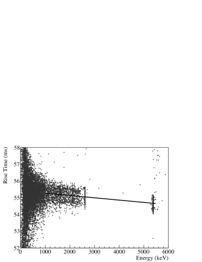
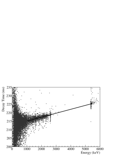
   Figure 5: Pulse shape parameters versus energy. The rise time (a) and the decay time (b) are anti-correlated and correlated with energy respectively.

2. The amplitude of the pulse depends on the base temperature. In figure 6 the amplitude of 5407$\mathrm{\,keV}$ events is plotted with respect to the pulse baseline, showing a clear anti-correlation. The temperature variation of the baseline is about $40\mathrm{\,\mu K}$, which corresponds to an energy variation of the crystal of about $400\mathrm{\,keV}$. The pulse amplitude changes by about $1\%$, worsening the resolution of the detector. This effect can be partially corrected by applying a calibrated heat source to the detector Alessandrello et al. (1998); Arnaboldi et al. (2003) and stabilizing the base temperature Arnaboldi et al. (2005).

   

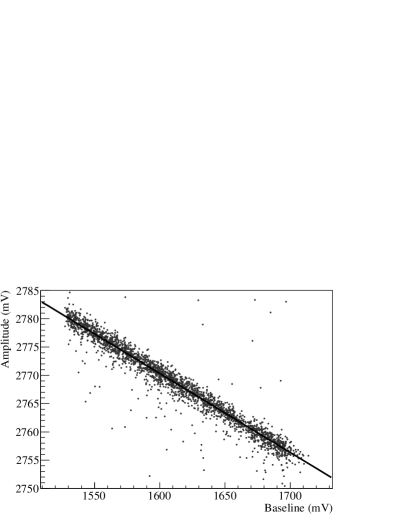
   Figure 6: Amplitude of 5407$\mathrm{\,keV}$ pulses versus baseline. A change in the bolometer temperature also changes its response, worsening the resolution.

3. The amplitude dependence on energy is not linear, and is usually parameterized with a polynomial function. The deviation from linearity of the data is estimated using a linear calibration function

   $$\rm{Energy}=\rm{constant}\cdot\rm{Amplitude}$$ (2)

   and then the difference between the energy estimated with this function and the nominal one is computed. The residuals evaluated on the peaks labeled in Fig. 4 are shown in Fig. 7. The 5407$\mathrm{\,keV}$ line is not included, since $\alpha$ particles have a quenching factor different from $\gamma$ and $\beta$ particles Alessandrello et al. (1998). If the true calibration function were a line, the residuals would be much smaller than the energy resolution, that is of order 5$\mathrm{\,keV}$ FWHM. The data, however, clearly indicate that a line is not sufficient to describe the calibration function.

   

   Figure 7: Residuals obtained using a linear calibration function. The difference $\Delta E$ between the estimated energy and the nominal one is not compatible with zero, considering that the energy resolution is $\sim 5\mathrm{\,keV\,FWHM}$. The error bars refer to the uncertainty on the estimated peak position, that depends on the FWHM and on the number of events $N$ in the peak as ${\rm FWHM}/(2.35\sqrt{N})$.

IV Thermistor and biasing circuit models

The detector contains many elements that can generate the observed non-linearities. The heat capacitance and conductance of the crystal, of the Teflon supports and of the thermistor, all depend on the temperature. The crystal capacitance for example is not linear in temperature, as it follows the Debye law ($C\propto T^{3}$). The problem of modeling the response function is that not all elements can be measured with satisfactory precision. In particular the contact heat conductance between the crystal and its supports changes with the detector configuration and the heat conductance of the glue varies from bolometer to bolometer because of the weak reproducibility of the glue deposition. In principle the knowledge of all parameters is needed if we want to predict the response function. However, we can narrow our focus to the aspects of the physical system which produce the dominant contributions to the non-linearity. In this section we will develop a model of the thermistor response and of the biasing circuit. It will be shown that they can account for all the observable non-linearities, without using any thermal model.

First we have to extract the temperature of the thermistor from the measured resistance. Unfortunately we cannot use Eq. (1), since parameters $R_{0}$ and $T_{0}$ cannot be measured with precision. This is due to the fact that when the thermistor is attached to the crystal, the glue stresses the device modifying its features in an unpredictable way. However, since we are interested in measuring energy depositions and not absolute temperatures, we can just evaluate the temperature variation. The resistance variation, $\Delta R$, in terms of the temperature variation, $\Delta T$, can be approximated as:

$$\Delta R(\Delta T) =R(T+\Delta T)-R(T)$$

$$\simeq R(T)\left[\exp(-\eta\Delta T/T)-1\right]$$ (3)

where:

$$\eta=\left|\frac{d\log{R}}{d\log T}\right|={\gamma}\log\frac{R(T)}{R_{0}}$$ (4)

is the sensitivity of the thermistor and its value is of order 10. The reason for expanding the exponential argument in terms of $\Delta T/T$ instead of the entire formula is that it provides a better approximation. The approximation is valid for $\Delta T/T\ll 1$, or, in terms of particle energy, for $E\ll C\,T$. Since $C\,T$ is of order $100\mathrm{\,MeV}$ ($C$ and $T$ are about 10$\mathrm{\,MeV/mK}$ and 10$\mathrm{\,mK}$ respectively), the approximation holds in the entire energy range . The advantage of Eq. (IV) is that it allows $\Delta T$ to be extracted from $\Delta R$ using a measurable parameter (the resistance $R(T)$) and that the unmeasurable parameter ($\eta/T$) is just a scale factor. In order to simplify the notation we define $\sigma=\eta/T$ for future calculations.

In the next section we will put in evidence the non-linearities generated by Eq. (IV) making the following assumptions:

1. The temperature response of the detector after an energy deposition $E$ can be parametrized as

   $$\Delta T(t,E)=A(E)\,U(t)$$ (5)

   where $U(t)$ is a function representing the time evolution of the temperature pulse and $A(E)$ is the amplitude of the pulse, which depends on the energy deposited.

2. The pulse shape $U(t)$ is independent of the energy and has unitary amplitude.

3. The amplitude $A(E)$ is proportional to the energy.

4. Both $A$ and $U$ are independent of the baseline temperature (the temperature before the energy deposition).

The properties of the resistance signal, $\Delta R(t)$, obtained under these assumptions will be compared with the measured voltage signal, assuming that the biasing circuit does not add non-linearities.

The dependence of the shape parameters on energy (see Fig. 5) is obtained computing the time derivative of the signal $\Delta R(t,E)$ normalized to its amplitude $A_{R}(E)$:

$$\frac{\Delta R^{\prime}(t,E)}{A_{R}(E)} =-\frac{\exp[-\sigma A(E)\,U(t)]\,\sigma\,A(E)\,U^{\prime}(t)}{\exp[-\sigma A(E)]-1}$$

$$\simeq U^{\prime}(t)\left[1-\sigma A(E)\,U(t)\right]\,,$$ (6)

where $A_{R}(E)=\min_{t}[\Delta R(t,E)]$ (since $\Delta R(t,E)$ is a negative signal) and $U^{\prime}(t)$ is the time derivative of $U(t)$. This expression indicates that the signal is slower when the energy increases, the same effect seen on the decay time of the pulse. This equation does not explain the behavior of the rise time, that is dominated by the biasing circuit (see later in the text).

The dependence of the pulse amplitude on baseline is also straightforward to derive. The resistance variation of the pulse baseline depends on the temperature according to the expression:

$$\Delta R_{B}=R(T)\left[\exp(-\sigma\Delta T_{B})-1\right]$$ (7)

where $\Delta T_{B}$ is the temperature variation with respect to $T$. When energy is released, the temperature increases by $A(E)$, and the total resistance change will be:

$$\Delta R_{Tot}=R(T)\left[\exp(-\sigma(\Delta T_{B}+A(E)))-1\right].$$ (8)

The amplitude of the pulse, however, is computed with respect to the baseline. In terms of resistance variation it will be:

$$A_{R}(E,\Delta R_{B}) =\Delta R_{Tot}-\Delta R_{B}$$

$$\simeq\left[1+\frac{\Delta R_{B}}{R(T)}\right]A_{R}(E,\Delta R_{B}=0)\,.$$ (9)

Recalling that a baseline increase in Volts corresponds to a resistance decrease, this expression describes the anti-correlation of the pulse amplitude with its baseline (see Fig. 6).

The non-linearity of the calibration function comes directly from Eq. (IV). If we assume that $A(E)=E/C$, the pulse amplitude $A_{R}(E)$ at the second order increases with energy as:

$$A_{R}(E)=R(T)\left[-\sigma\frac{E}{C}+\left(\sigma\frac{E}{C}\right)^{2}+\ldots\right]\,.$$ (10)

Recalling that the signal in Volts has opposite sign of the resistance variation, this is the same behavior of Fig. 7.

The thermistor formula (IV) explains at this point at least qualitatively all the data, except for the rise time of the pulse. The calculations showed in fact that the shape parameters should get slower with amplitude. The rise time, however, becomes faster (see Fig. 5). This effect can be generated by the biasing circuit, whose parasitic capacitance, $c_{p}$, introduces a cutoff that varies with the pulse amplitude. We solve the circuit of Fig. 2 approximately, using $R_{L}\gg R$ and $R_{L}\gg\Delta R(t)$. We have that the voltage signal $\Delta V(t)$ in terms of the resistance signal $\Delta R(t)$ can be expressed as:

$$\Delta V(t)+\left[R(T)+\Delta R(t)\right]c_{p}\Delta V^{\prime}(t)=-\frac{V_{B}}{R_{L}}\Delta R(t),$$ (11)

where $\Delta V(t)=V(t)-V_{R}$, and $V_{R}$ is the voltage corresponding to the static resistance $R(T)$: $V_{R}=-V_{B}\,R(T)/[R(T)+R_{L}]$. Expression (11) has the form of a low pass filter whose cutoff, $[c_{p}(R(T)+\Delta R(t))]^{-1}$, depends on $\Delta R(t)$ and hence on its amplitude. The higher is the absolute value of the amplitude, the higher is the cutoff (since the amplitude is negative), making the voltage pulse faster. Since $R(T)c_{p}$ is of order 30$\mathrm{\,ms}$, this effect is visible only on the fast part of the voltage pulse (the rise time) and competes with the thermistor slowing down.

V Linearization of the response function

It has been shown that the behavior of the data can be explained assuming that the thermal response $\Delta T(t)$ does not depend on the energy released or on the variation of the baseline bolometer temperature. The non-linearities of the voltage signal seem to be generated by the thermistor and by the biasing circuit. Here we derive an algorithm to extract a signal proportional to $\Delta T(t)$, and we will test its performance on data.

First the variation of the thermistor resistance is extracted from $V(t)$ solving the biasing circuit of Fig. 2:

$$\Delta R(t)=-\frac{\Delta V(t)[R(T)+R_{L}]+R_{L}\,R(T)\,c_{p}\Delta V^{\prime}(t)}{\Delta V(t)+R_{L}c_{p}\Delta V^{\prime}(t)+V_{B}\,R_{L}/[R(T)+R_{L}]}\,,$$ (12)

where $\Delta V(t)$ is defined in the previous section. Then from Eq. (IV) the quantity $\Delta S(t)=\sigma\,\Delta T(t)$ is computed:

$$\Delta S(t)=-\log\left[1+\frac{\Delta R(t)}{R(T)}\right]\,.$$ (13)

The advantage of this algorithm is that it depends on parameters that can be measured with sufficient precision. These parameters are the static bolometer resistance $R(T)$ and the voltage across it $V_{R}$, the load resistance $R_{L}$, the parasitic capacitance $c_{p}$ and the bias voltage $V_{B}$. The unknown quantities have been hidden in a common scale factor $(\sigma)$, that is not relevant if we are only interested in removing the non-linearities. This algorithm has been implemented as a digital filter on the voltage data sampled by the ADC. The derivative of $\Delta V$ has been computed as $\Delta V^{\prime}_{i}=(V_{i+1}-V_{i-1})/(2\,\Delta t)$, where $i$ is the sample index and $\Delta t$ is the sampling period. A comparison between the original $\Delta V(t)$ signal and the same signal transformed into $\Delta R(t)$ and $\Delta S(t)$ is shown in Fig. 8.

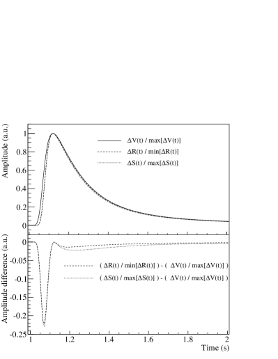
Figure 8: Comparison between the original $\Delta V(t)$ signal generated by a 2615 keV $\gamma$ particle, and the same signal transformed into $\Delta R(t)$ and $\Delta S(t)$. The $\Delta R(t)$ signal is faster than the $\Delta V(t)$ one, because the low pass filter of the biasing circuit has been deconvoluted. The $\Delta S(t)$ signal is even faster since the thermistor slowing down effect has been removed.

The $\Delta S$ data have been analyzed with the same analysis procedure applied on $\Delta V$ data. The features of the transformed signal are:

1. The shape of the pulse has a much weaker dependence on energy. The correction is particularly evident on the decay time, where the correlation has been reduced by a factor 6 (see Fig. 9).

   

   

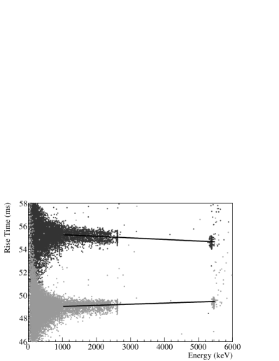
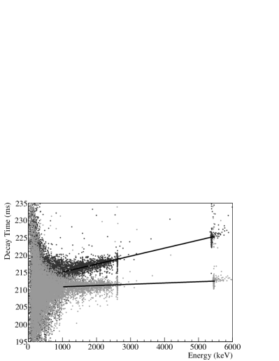
   Figure 9: Pulse shape parameters versus energy. The $\Delta S$ data (light gray) are less dependent on energy than $\Delta V$ data (dark gray), the correction is particularly effective on the decay time (b). The rise time (a) of $\Delta S$ data is faster, because the low pass filter of the biasing circuit has been deconvoluted.

2. The amplitude dependence on the baseline is removed. The slope is reduced by a factor 20 (see Fig. 10).

   

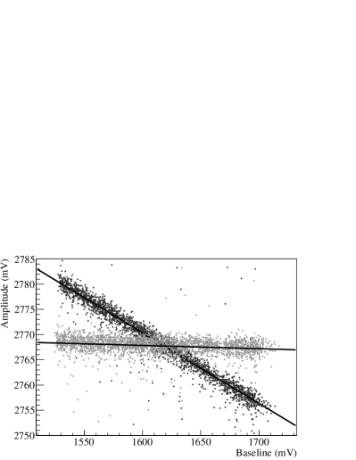
   Figure 10: Amplitude of 5407$\mathrm{\,keV}$ pulses versus baseline. The $\Delta S$ data (light gray) are less correlated with the baseline than $\Delta V$ data (dark gray). The ratio of the slopes is about 20.

3. The calibration function is a line. The comparison of the residuals clearly indicates that the non-linearities of the calibration function have been removed (see Fig. 11).

   

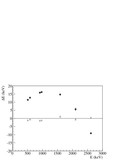
   Figure 11: Residuals of the linear calibration function. The residuals of $\Delta S$ data (light gray) are very close to zero and have no trend compared to $\Delta V$ data (dark gray).

In conclusion, the model we have developed describes nearly all the observable non-linearities of the response function. It relies only on fixed parameters, that can be measured on the detector. The data transformed with an algorithm derived from the model provide a much more linear response function, improving the operation and the data analysis of these detectors.