Transitions in turbulent rotating Rayleigh-Bénard convection

Abstract

Numerical simulations of rotating Rayleigh-Bénard convection are presented for both no slip and free slip boundaries. The goal is to find a criterion distinguishing convective flows dominated by the Coriolis force from those nearly unaffected by rotation. If one uses heat transport as an indicator of which regime the flow is in, one finds that the transition between the flow regimes always occurs at the same value of a certain combination of Reynolds, Prandtl and Ekman numbers for both boundary conditions. If on the other hand one uses the helicity of the velocity field to identify flows nearly independent of rotation, one finds the transition at a different location in parameter space.

1 Introduction

At least two flow regimes exist in rotating Rayleigh-Bénard convection in plane layers: Near the onset of convection, the nonlinear advection terms are small and the Coriolis force dominates the dynamics, provided the Ekman number is small enough. The controlling effect of the Coriolis force is the distinguishing feature of the first regime. If the Rayleigh number is increased at fixed Ekman and Prandtl numbers, the advection term in the Navier-Stokes equation becomes larger than the Coriolis term (which is linear in velocity) so that rotation becomes irrelevant and the flow behaves as if rotation was absent. This defines the second regime. For the purpose of predicting the Nusselt number, it was found useful in Schmitz and Tilgner (2009) to introduce a transitional regime into the classification, in which the Nusselt number obeys a power law different from those observed in the two other regimes. There is an ongoing debate concerning the parameters at which the transition between the first and second regimes occurs (Rossby (1969); Aurnou (2007); Liu and Ecke (2009); King et al. (2009); Schmitz and Tilgner (2009)). While there is by now ample evidence that the naive criterion that the Rossby number equals one at the transition is inadequate, there is no agreement on what the correct criterion is. Recently, it was shown by King et al. (2009) that experimental heat flux data are compatible with the idea that the flow is in one regime or the other depending on whether the thermal boundary layer is thicker than the Ekman layer or vice versa. A numerical study by Schmitz and Tilgner (2009) avoided Ekman boundary layers by employing stress free boundary conditions. A transition between the two regimes still occurs and an analysis of the asymptotic behavior of the Nusselt number leads to a transition criterion based upon a combination of the Reynolds, Prandtl and Ekman numbers.

The present paper follows up on the numerical simulations presented in Schmitz and Tilgner (2009) and intends to answer two questions: First, how important are the boundary conditions? Is the criterion found in Schmitz and Tilgner (2009) still relevant for no slip boundaries? And second, is the classification of a given flow into the different regimes independent of the quantity used for that classification? Both Schmitz and Tilgner (2009) and King et al. (2009) classified flows according to their Nusselt number. Here, we will also look at a quantity derived from the velocity field which is important for the dynamo effect, namely the helicity.

2 The mathematical model

A plane layer of thickness $d$, filled with fluid of kinematic viscosity $\nu$, thermal diffusivity $\kappa$, and thermal expansion coefficient $\alpha$ rotates with angular velocity $\Omega$ about the $z-$axis. This axis is perpendicular to the layer. Gravitational acceleration $g$ is pointing in the negative $z-$direction. The temperatures of the top and bottom boundaries are fixed at $T_{0}$ and $T_{0}+\Delta T$, respectively. These two boundaries are assumed to be either free slip or no slip, whereas periodic boundary conditions are applied in the $x-$ and $y-$directions. The equations of evolution are made non-dimensional by using $d^{2}/\kappa$, $d$ and $\Delta T$ for units of time, length, and temperature, respectively. These equations then become within the Boussinesq approximation for the dimensionless velocity $\bm v(\bm r,t)$ and temperature $T(\bm r,t)$:

$$\partial_{t}\bm v+(\bm v\cdot\nabla)\bm v+2\frac{Pr}{Ek}\hat{\bm z}\times\bm v=-\nabla p+Pr~{}\nabla^{2}\bm v+Ra~{}Pr~{}T\hat{\bm z}$$ (1)

$$\nabla\cdot\bm v=0$$ (2)

$$\partial_{t}T+\bm v\cdot\nabla T=\nabla^{2}T$$ (3)

$\hat{\bm z}$ is the unit vector in $z-$direction and $p$ collects the pressure and the centrifugal acceleration. The boundary conditions state in terms of the adimensional quantities that $T(z=0)=1$, $T(z=1)=0$, and free slip boundary conditions require that $v_{z}=\partial_{z}v_{x}=\partial_{z}v_{y}=0$ at both $z=0$ and $z=1$, whereas $v_{x}=v_{y}=v_{z}=0$ for no slip boundaries. Three independent dimensionless control parameters appear: The Rayleigh number $Ra$, the Ekman number $Ek$, and the Prandtl number $Pr$. They are defined by:

$$Ra=\frac{g\alpha\Delta Td^{3}}{\kappa\nu}~{}~{}~{},~{}~{}~{}Ek=\frac{\nu}{\Omega d^{2}}~{}~{}~{},~{}~{}~{}Pr=\frac{\nu}{\kappa}.$$ (4)

The Reynolds number $Re$ and the Nusselt number $Nu$ are computed as:

$$Re=\frac{1}{Pr}\sqrt{\frac{1}{V}\int\overline{\bm v^{2}}dV}~{}~{}~{},~{}~{}~{}Nu=-\frac{1}{A}\int\overline{\partial_{z}T}dA.$$ (5)

The overbar denotes average over time and the integrals extend over the computational volume $V$ for $Re$ and over the surface $A$ of either the top or the bottom boundary for $Nu$.

The equations of motion were solved with the same spectral method as used in Schmitz and Tilgner (2009). Resolutions reached up to 129 Chebychev polynomials for the discretization of the $z-$coordinate and $256\times 256$ Fourier modes in the $(x,y)-$plane. The periodicity lengths along the $x-$ and $y-$ directions were always chosen to be identical. Since the typical size of flow structures varies considerably as a function of the control parameters in rotating convection, it is not useful to use a single aspect ratio throughout all simulations, where the aspect ratio is defined as the ratio of the periodicity length in the $(x,y)-$plane and the layer height. The aspect ratio was adjusted for each $Ek$ to fit at least 8 columnar vortices along both the $x-$ and $y-$directions at the onset of convection, and kept constant as $Pr$ and $Ra$ were varied.

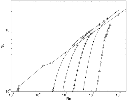
Figure 1: $Nu$ as a function of $Ra$ for no slip boundaries at $Pr=7$ and $Ek=3.4\times 10^{-3}$ (x), $Ek=1.7\times 10^{-3}$ (+), $Ek=8.7\times 10^{-4}$ (*), $Ek=4.7\times 10^{-4}$ ($\bullet$), and $Ek=2\times 10^{-4}$ ($\Delta$). The open circles are for zero rotation.

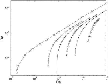
Figure 2: $Re$ as a function of $Ra$ for no slip boundaries at $Pr=7$ and $Ek=3.4\times 10^{-3}$ (x), $Ek=1.7\times 10^{-3}$ (+), $Ek=8.7\times 10^{-4}$ (*), $Ek=4.7\times 10^{-4}$ ($\bullet$), and $Ek=2\times 10^{-4}$ ($\Delta$). The open circles are for zero rotation.

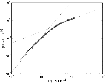
Figure 3: $(Nu-1)Ek^{1/3}$ as a function of $Re\,Pr\,Ek^{1/2}$ for the same data and with the same symbols as in figs. 1 and 3. The dashed lines are power laws with exponents 2 and 2/3. The points inside the interval delineated by the two vertical lines reappear in figure 4.

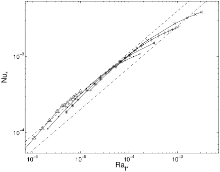
Figure 4: $Nu_{*}$ as a function of $Ra_{f*}$. The symbols have the same meaning as in fig. 1. This figure contains only those data points which lie in the interval marked by vertical lines in fig. 3. The straight lines indicate the functions $Nu_{*}=0.11\cdot Ra_{f*}^{0.55}$ (lower, dot dashed line) which fits well to simulations with free slip boundaries, and $Nu_{*}=0.17\cdot Ra_{f*}^{0.55}$ (upper, dashed line).

3 No slip boundaries

Computations for no slip boundaries are much more demanding than in the free slip case. That’s why the parameter range covered by the data in figure 1 is smaller than in the equivalent figure in Schmitz and Tilgner (2009). Nonetheless, the data suffice to show that the behavior is essentially the same for both types of boundary conditions. Figure 1 shows $Nu(Ra)$ for no slip boundary conditions. One recognizes the well known pattern of a delayed onset of convection followed by a steep rise. $Nu$ in the rotating flow may even exceed its value for zero rotation for no slip boundary conditions (Zhong et al. (2009)). The delayed onset of convection is also visible in the graph of Reynolds number versus Rayleigh number (figure 2).

Figure 3 uses a data reduction motivated by the results for free slip boundary conditions . Some of the arguments of Schmitz and Tilgner (2009) are recapitulated here to make the paper self-contained. Low values of ${Re}\,{Pr}\,{Ek}^{1/2}$ correspond to laminar flows near the onset of convection. Forming the dot product of eq. (1) and $\bm v$, integrating over the whole volume and averaging over time, one finds

$$\epsilon=({Nu}-1){Ra}$$ (6)

where $\epsilon=\frac{1}{V}\int<(\partial_{i}v_{j})(\partial_{i}v_{j})>dV$ is the adimensional average dissipation rate of kinetic energy. In a laminar flow, one expects $\epsilon\propto({Re}\,{Pr})^{2}/\lambda^{2}$, where $\lambda$ is a characteristic length scale of the flow. For ${Pr}>0.676$, convection starts at a critical Rayleigh number ${Ra}_{c}$ obeying ${Ra}_{c}\propto{Ek}^{-4/3}$ and forms stationary cells of size $\lambda_{c}$ with $\lambda_{c}\propto{Ek}^{1/3}$ (Chandradekhar (1961)). Eq. (6) becomes ${Ek}^{-2/3}{Re}^{2}{Pr}^{2}\propto({Nu}-1){Ra}$. Close to onset, ${Ra}\approx{Ra}_{c}$ and therefore $({Nu}-1)\propto{Re}^{2}{Pr}^{2}{Ek}^{2/3}$. For large values of ${Re}\,{Pr}\,{Ek}^{1/2}$, one should approach the non-rotating case and find a law independent of ${Ek}$. There is no reliable theory for convection far from the onset so that we have to rely on numerical results. Simulations show that $({Nu}-1)\propto({Re}\,{Pr}\,)^{2/3}$ for zero rotation. Both asymptotes, near onset and far from it, become straight lines in a logarithmic plot of $({Nu}-1){Ek}^{1/3}$ vs. ${Re}\,{Pr}\,{Ek}^{1/2}$.

Figure 3 shows $(Nu-1)Ek^{1/3}$ as a function of $Re\,Pr\,Ek^{1/2}$ for no slip boundary conditions and should be compared with figure 2 of Schmitz and Tilgner (2009). The dashed lines have the slopes of the asymptotes which $(Nu-1)Ek^{1/3}$ has to follow either in the limit of large Rayleigh numbers (when rotation plays no role) or near the onset of convection. The prefactors in these power laws are obtained from best fits to the simulations with free slip boundary conditions of Schmitz and Tilgner (2009) so that a direct comparison is possible with the results of computations with no slip boundary conditions shown by points in the figure. It is seen that both boundary conditions have asymptotes with the same exponents. Most importantly, for both boundary conditions, the crossing of the two asymptotes near $Re\,Pr\,Ek^{1/2}=2$ separates the convection dominated by rotation from the convection virtually unaffected by rotation.

It is noteworthy that in the no slip case of figure 3, the asymptotes provide us with reasonably good fits throughout the entire parameter range. In the case of free slip boundary conditions in Schmitz and Tilgner (2009), the interval $1/2<Re\,Pr\,Ek^{1/2}<10$ (indicated by vertical bars in figure 3) required special treatment. It turned out to be useful to introduce nondimensional parameters independent of molecular diffusivities already discussed in previous work (Christensen (2002); Aurnou (2007)): $Nu_{*}=Nu\,Ek/Pr=Q/(\rho c_{p}\Delta T\Omega d)$ and $Ra_{f*}=Nu_{*}\,Ra\,Ek^{2}/Pr=(g\alpha Q)/(\rho c_{p}\Omega^{3}d^{2})$, where $\rho$ denotes density and $c_{p}$ heat capacity. An envelope to the data in the interval $1/2<Re\,Pr\,Ek^{1/2}<10$ is given by $Nu_{*}=0.11\cdot Ra_{f*}^{0.55}$ for free slip boundaries. Figure 4 shows that a similar conclusion holds for no slip boundaries after a change in the prefactor: $Nu_{*}=0.17\cdot Ra_{f*}^{0.55}$ is more appropriate in this case.

4 Free slip boundaries: Helicity

In order to quantify the influence of rotation on the flow structure, we investigate the helicity $H$, or more precisely the correlation between vorticity and velocity, defined by:

$$H=\frac{(\nabla\times\bm v)\cdot\bm v}{|\nabla\times\bm v|\,|\bm v|}.$$ (7)

This correlation is now averaged over horizontal planes, and ideally over time. However, helicity was not saved during the production runs so that it had to be deduced from single snapshots. Assuming ergodicity of the flow, the spatial average replaces to some extent the temporal average. The noise in the figures below is low enough so that further simulations did not seem warranted. The average helicity $\langle H\rangle$, defined by

$$\langle H\rangle=\frac{1}{A}\int dx\int dy\,H$$ (8)

where $A$ is the area of a horizontal plane, is shown in figure 5. As expected (Chandradekhar (1961)), rotation introduces helicity of one sign in one half of layer and of the opposite sign in the other half ($z=0.5$ is not an exact plane of symmetry in figure 5 because of the missing time average). As $Ra$ increases, the advection term increases compared with the Coriolis term and the helicity decreases. The maximum of $\langle H\rangle$ is reached at a point at a smaller and smaller distance from the boundaries as $Ra$ is increased. Helicity is induced by the presence of the boundaries because they force in- and outflow out of departing or arriving plumes which is spun up by the Coriolis force. When turbulence tends to destroy the correlation between vorticity and velocity present in helical structures, it is easiest to do so away from the walls.

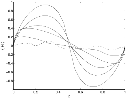
Figure 5: Average helicity $\langle H\rangle$ as a function of height $z$ for no slip boundaries, $Ek=2\times 10^{-3}$ and $Pr=7$. In going from the curve drawn with a continuous line of largest amplitude to the one with smallest amplitude, the Rayleigh number is $Ra=1.0\times 10^{5}$, $2.0\times 10^{5}$, $5.0\times 10^{5}$, $1.0\times 10^{6}$, and $1.0\times 10^{7}$. The dashed curve is for $Ra=1.0\times 10^{8}$.

A suitable global measure for the influence of the rotation on the velocity field is the rms fluctuation in $\langle H\rangle(z)$, i.e.

$$H_{rms}=\int_{0}^{1}\langle H\rangle^{2}dz.$$ (9)

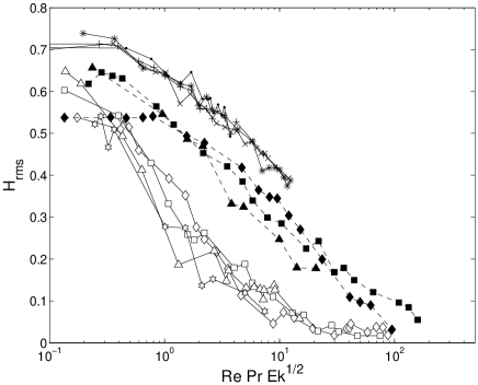
Figure 6: $H_{rms}$ as a function of $Re\,Pr\,Ek^{1/2}$. The filled symbols are for $Pr=7$ and the empty symbols for $Pr=0.7$. The Ekman numbers are $Ek=2.0\times 10^{-2}$ (diamonds), $2.0\times 10^{-3}$ (squares), $2.0\times 10^{-4}$ (triangles) and $2.0\times 10^{-5}$ (stars). The remaining symbols indicate no slip boundaries and $Ek=1.7\times 10^{-3}$ (x), $Ek=8.7\times 10^{-4}$ (+), $Ek=4.7\times 10^{-4}$ (*), and $Ek=2\times 10^{-4}$ ($\bullet$), all for $Pr=7$.

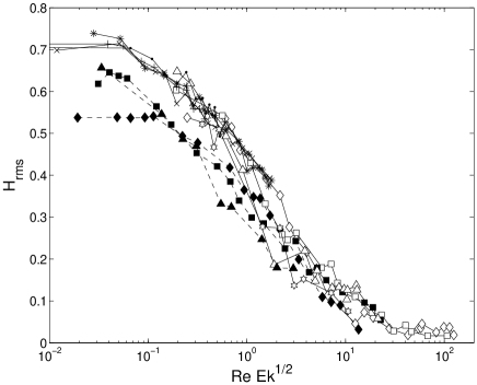
Figure 7: $H_{rms}$ as a function of $Re\,Ek^{1/2}$. The symbols are the same as in figure 6.

Figure 6 gives $H_{rms}$ as a function of $Re\,Pr\,Ek^{1/2}$. There is a reasonable collapse of the data for a given $Pr$, which shows that the combination $Re\,Pr\,Ek^{1/2}$ captures the right $Re$ and $Ek$ dependences, but the points for different $Pr$ do not fall on top of each other. However, if one plots $H_{rms}$ as a function of $Re\,Ek^{1/2}$, one again obtains a good collapse of the data points, at least at large $Re\,Ek^{1/2}$ (see figure 7). Within the noise on $H_{rms}$, the flow is indistinguishable from nonrotating convection for $Re\,Ek^{1/2}>50$. The transition criteria are thus not identical when based on the Nusselt number or on the helicity. The transition occurs at a certain value of $Re\,Pr\,Ek^{1/2}$ in as far as heat flux is concerned, and at a certain value of $Re\,Ek^{1/2}$ for helicity.

5 Discussion and conclusion

It was shown in section 3 that according to the Nusselt number, $Re\,Pr\,Ek^{1/2}=2$ separates flows dominated by the Coriolis force from flows unaffected by rotation for both types of boundary conditions, free slip and no slip. The combination $Re\,Pr\,Ek^{1/2}$ can be recognized as the Peclet number based on the thickness of the Ekman layer. This interpretation is not directly useful, however. It is not clear why this Peclet number should matter for the heat flux, because the heat flux is crossing diffusively the velocity boundary layer in which velocity and temperature gradient are mostly perpendicular to each other so that $\bm v\cdot\nabla T=0$ and $\bm v$ does not enter the temperature equation (3) within the boundary layers. In addition, there is no Ekman layer for free slip boundaries, and yet, the transition occurs at the same values of the control parameters.

One may argue that a length scaling as $Ek^{1/2}$ is not completely foreign to free slip boundaries, either. Hide (1964) calculates a velocity boundary layer thickness in $Ek^{1/2}$ near a free slip boundary provided that the density of the fluid varies along the surface. This cannot be the case within the Boussinesq approximation on an isothermal boundary, so that this mechanism cannot create a length in $Ek^{1/2}$ in our simulations. Julien et al. (1996) also find an $Ek^{1/2}$ layer in the velocity field if the thermal boundary layer thickness varies laterally. Their calculation posits a lateral temperature variation which is not advected by the horizontal velocity, so that this result is not directly applicable to self-consistent simulations. Nonetheless, these analytical calculations are motivation enough to scan the velocity profiles obtained from the numerical simulations for a length scaling as rapidly as $Ek^{1/2}$ as a function of the Ekman number. However, no such length could be found in the case of free slip boundaries.

As section 4 has shown, the transition from a flow dominated by rotation to a flow unaffected by rotation is not well defined, anyway. The transition occurs at different values of the control parameters depending on whether the classification is based on the Nusselt number or on the helicity of the velocity field. The helicity is down to negligible magnitude for $Re\,Ek^{1/2}>50$. We will now apply this result to the Earth’s core. Most data in this paper were obtained for free slip boundaries, but the close agreement between free slip and no slip boundaries found here encourages us to apply the transition criteria to the Earth’s core nonetheless. For the Earth’s core, the generally accepted values of $\nu=5\times 10^{-7}m^{2}/s$, $\Omega=7.29\times 10^{-5}s^{-1}$ and a typical flow velocity of $5\times 10^{-4}m/s$ lead to $Re\,Ek^{1/2}=82$. This estimate casts doubts on the picture of a geodynamo operating as an $\alpha^{2}-$dynamo with an $\alpha-$effect due to the helicity of the flow.

This work was supported by the Deutsche Forschungsgemeinschaft (DFG).

References

- Aurnou (2007) Aurnou, J.M., Planetary core dynamics and convective heat transfer scaling. Geophys. Astrophys. Fluid Dynamics 2007, 101, 327–345.
- Chandradekhar (1961) Chandradekhar, S., Hydrodynamic and Hydromagnetic Stability, 1961 (Oxford: Oxford University Press).
- Christensen (2002) Christensen, U.R., Zonal flow driven by strongly supercritical convection in rotating spherical shells. J. Fluid Mech. 2002, 470, 115–133.
- Hide (1964) Hide, R., The viscous boundary layer at the free surface of a rotating baroclinic flow. Tellus 1964, A 16, 523–529.
- Julien et al. (1996) Julien, K., Legg, S., McWilliams, J. and Werne, J., Rapidly rotating turbulent Rayleigh-Bénard convection. J. Fluid Mech. 1996, 322, 243–273.
- King et al. (2009) King, E.M., Stellmach, S., Noir, J., Hansen, U. and Aurnou, J.M., Boundary layer control of rotating convection systems. Nature 2009, 457, 301–304.
- Liu and Ecke (2009) Liu, Y. and Ecke, R., Heat transport measurements in turbulent rotating Rayleigh-Bénard convection. Phys. Rev. E 2009, 80, 036314.
- Rossby (1969) Rossby, H.T., A study of Bénard convection with and without rotation. J. Fluid Mech. 1969, 36, 309–335.
- Schmitz and Tilgner (2009) Schmitz, S. and Tilgner, A., Heat transport in rotating convection without Ekman layers. Phys. Rev. E 2009, 80, 015305(R).
- Zhong et al. (2009) Zhong, J.Q., Stevens, R.J.A.M., Clercx, H.J.H., Verzicco, R., Lohse, D. and Ahlers, G., Prandtl-, Rayleigh-, and Rossby-Number Dependence of Heat Transport in Turbulent Rotating Rayleigh-Bénard Convection. Phys. Rev. Lett. 2009, 102, 044502.