Testing non-locality of single photons using cavities

Abstract

A scheme is formulated for testing nonlocality of single photons by considering the state of a single photon that could be located within one of two spatially separated cavities. The outcomes of four experiments on this state involving the resonant interactions of two-level atoms with these cavities and a couple of other auxiliary ones is shown to lead to a contradiction with the criterion of locality.

Introduction.—

In classical physics two distantly separated particles obey Einstein’s locality, i.e., the outcome of a measurement on one of the particles does not effect what is being measured on the other. On the other hand, the nonlocal nature of the quantum world has for long attracted deep attention among physicists ever since the famous EPR paper EPR . Specifically, though information cannot be transmitted between spacelike separated observers, any realistic hidden variable theory capable of reproducing the results of quantum theory would have to be nonlocal. A precise identification of nonlocality as a crucial ingredient of distinction between classical and quantum physics was performed by Bell in his seminal paper Bell . The violation of Bell’s inequality which has been demonstrated in a number of experiments Expt1 , underlines the nonlocality of quantum states of two or more particles.

If nonlocality is to be regarded as an inherent feature of the quantum world, it is difficult to understand why this feature should be manifest only at the level of two or more particles. A quantum state should reveal its nonlocal property irrespective of the number of particles associated with it. At the field theoretic level particles are regarded as excitations of the quantum vacuum, and there is no fundamental difference between a single particle excitation, and a two-particle one. Specifically, a single particle should also be able to exhibit nonlocality under particular circumstances, as was indeed indicated by Einstein in 1927 solvay while presenting the collapse of a single particle wave packet to a near eigenstate as an example of quantum nonlocality. It took more than half a century since then for the concept of nonlocality of single particles to be more precisely formulated by Tan, Walls and Collett TWC through the idea that measurements made on two output channels from a source could violate locality even if one particle is emitted from the source at a time. However, additional assumptions in this proposal narrowed down the scope of its implementation considerably twc2 . In this context it may be noted that a single particle could carry two or more degrees of freedom (i.e., the spatial and polarization variables in case of a photon), and it is possible to demonstrate the violation of Bell-type inequalities in such cases signifying the violation of non-contextuality at the level of a single particle home . Further, entanglement between different degrees of freedom of the same particle could be exploited as resource for performing information processing tasks pramanik . On the other hand, the establishment of nonlocality at the level of a single particle has still remained a subtle issue.

A demonstration of quantum nonlocality for two entangled particles without the use of mathematical inequalities, was formulated by Hardy hardy0 . Subsequently, he proposed a scheme to demonstrate the nonlocality of single photons Hardy without the supplementary assumptions made in the work of Tan, Walls and Collett TWC . Hardy’s scheme was criticized for not being experimentally realizable by Greenberger, Horne and Zeilinger (GHZ) ghz who in turn proposed their own scheme which required additional particles for implementation. Here again, the issue of whether nonlocality is purely a multipartite effect could not be settled since it could be debated that the additional particles were responsible for introducing nonlocality into the system. Another proposal showing an incompatibility between quantum mechanics and any local deterministic ontological model in terms of particle coordinates was formulated for single photon states HA . Recently, Dunningham and Vedral DV have formulated a scheme for demonstrating nonlocality of single photons, overcoming several problems of earlier proposals. Their scheme which relies on the use of mixed states, is experimentally realizable, as claimed by the authors, but has still not been practically performed.

The notion of single particle nonlocality is of such conceptual importance in the physical interpretation of quantum theory, that it is worthwhile to think of more proposals in order to demonstrate it beyond any reasonable doubt. In this regard, it may be noted that as different from the case of nonlocality of two particles, single particle nonlocality has still not been conclusively demonstrated experimentally in a manner free of conceptual loopholes. Note here that an experiment performed earlier by Hessmo et al. hessmo for exhibiting single photon nonlocality was based on the schemes of Tan, Walls and Collett TWC and Hardy Hardy , and hence, not free of the conceptual problems raised by GHZ ghz and others DV . The scheme proposed by Dunningham and Vedral DV promises to circumvent those problems, but is yet to be experimentally implemented. With the above perspective, in this paper we present a proposal for demonstrating nonlocality of single photons inside cavities. The formulation of our scheme is based on atom-photon interactions in cavities, a well-studied arena on which controlled experiments have been performed for many years now Haroche . The ingredients for our proposal are two-level atoms, and single-mode high-Q cavities which are tuned to resonant transitions between the atomic levels. For example, the use of Rydberg atoms and microwave cavities in testing several fundamental aspects of quantum mechanics have been proposed majumdar , and various interesting experiments have been performed by keeping dissipative effects under control cavexpts .

Atom-cavity interaction dynamics.—

We consider the dynamics of a two-level atom passing through a cavity, which under the dipole and rotating wave approximations is described by the Jaynes-Cummings interaction Hamiltonian apr2 ; apr4

$$H^{I}(r)=G(r)(a\sigma_{+}+a^{\dagger}\sigma_{-}),$$ (1)

where $\sigma_{\pm}=\sigma_{x}\pm\sigma_{y}$ denote the Pauli spin operators for a two-level atom, and $a$, $a^{\dagger}$ are the annihilation and creation operators, respectively, for a photon in single mode cavity. The atom-field coupling strength may be expressed as $G(r)=\Omega_{0}(\hat{\bf{d}}_{eg}.\hat{\bf{e}}(r))f(r)$, where $\Omega_{0}$ is the peak atomic Rabi frequency, $\hat{\bf{d}}_{eg}$ is the orientation of the atomic dipole moment, and $\hat{\bf{e}}(r)$ is the direction of the electric field vector at the position of the atom. The profile $f(r)$ has an exponential envelop centered about the point in the atom’s trajectory that is nearest to the centre of the cavity, $r_{0}$ apr2 ; apr4 . Within this envelope, the field intensity oscillates sinusoidally, and for the fixed dipole orientation, variations in the relative orientation of the dipole and electric field gives a sinusoidal contribution, i.e.,

$$f(r)=e^{-\frac{|r-r_{0}|}{R_{def}}}\cos[\frac{\pi}{a_{l}}(r-r_{0})],$$ (2)

where $R_{def}$ defines the spatial extent of the mode which is at most a few times the lattice constant ($a_{l}$) for a strongly confined mode in a photonic band gap apr2 .

The atom-field state after an initially excited atom has passed through a cavity (which is initaially is in zero photon state) can be written as

$$|\phi_{e}\rangle=\alpha_{1}(t)|e\rangle|0\rangle+\alpha_{2}(t)|g\rangle|1\rangle,$$ (3)

where $\alpha_{1(2)}$ is the amplitude of the atom being in excited (ground) state and $t$ is the interaction time of the atom with the cavity, with

$$\alpha_{1}(t)=\cos[\int_{0}^{t}G(t^{\prime})dt^{\prime}]$$

$$\alpha_{2}(t)=\sin[\int_{0}^{t}G(t^{\prime})dt^{\prime}],$$ (4)

where we have replaced $(r-r_{0})$ by $(vt-b)$ with $v$ being the velocity of the atom in the cavity and $2b$ the effective length of interaction in the cavity. Setting the value of the interaction time $t=2b/v$, it is possible to obtain the exact expressions for the $\alpha_{1(2)}$, i.e.,

$$\alpha_{1(2)}=\cos(\sin)\Biggl{[}\frac{2a_{l}R_{def}\Omega_{0}ke^{-\frac{b}{R_{def}}}\left(a_{l}e^{\frac{b}{R_{def}}}+\pi R_{def}\sin\left(\frac{\pi b}{a_{l}}\right)-a_{l}\cos\left(\frac{\pi b}{a_{l}}\right)\right)}{v\left(a_{l}^{2}+\pi^{2}R^{2}_{def}\right)}\Biggr{]}$$ (5)

with $k=\hat{{\bf d}}_{eg}.\hat{{\bf e}}({\bf r})$, which can be chosen to take values from $0$ to $1$. Following apr4 , we henceforth set $a=624nm=R_{def}$, $b=10R_{def}$, and $\Omega_{0}=1.1\times 10^{10}rad/s$ in our calculations.

State preparation.—

The scheme for demonstrating nonlocality that we use in the present work is set up as follows. Let Alice and Bob be two spatially well separated parties who possess two cavities $C_{1}$ and $C_{2}$, respectively, an atom $a_{1}$ and a detector $D_{1}$ used in the state preparation process. Alice and Bob also possess an auxiliary cavity and an additional atom each, viz., $C_{4}$, $a_{3}$ and $C_{3}$, $a_{2}$ respectively, as well as two detectors $D_{2}$ and $D_{3}$, respectively, which they could either use or remove depending on the choice of the four different experiments they perform, as described below.

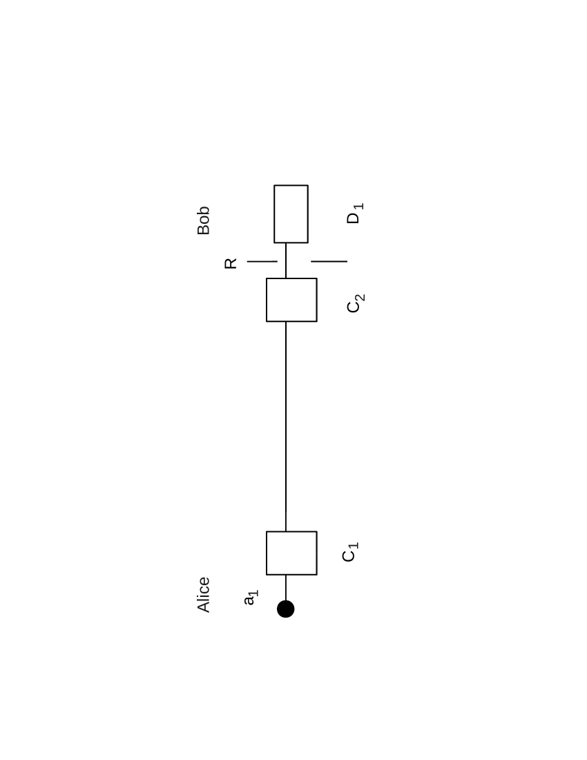
Figure 1: Experimental set up for creating the state given by Eq.(6). A two-level atom in its upper level traverses the cavities $C_{1}$ and $C_{2}$, before being detected in its lower level by the detector $D_{1}$. ($v_{a_{1}}=179\text{m/s}$, $k(a_{1};C_{1})=0.979$, $k(a_{1};C_{2})=1$).

We begin by describing the state preparation process for single photons (see Fig. 1), that we will use for the argument of nonlocality. Initially, the two cavities $C_{1}$ and $C_{2}$ are empty, i.e., in zero photon states denoted by $|0\rangle_{C_{1}}$ and $|0\rangle_{C_{2}}$. Now an atom (say atom-1), initially in the upper of its two possible levels, $|e\rangle_{a_{1}}$ traverses $C_{1}$ with flight time $t_{11}$ and then traverses $C_{2}$ with flight time $t_{12}$. The cavities are tuned to the resonant frequency for transitions between the upper and lower levels of the atom. Now, a $\frac{\pi}{2}R_{1}$ Ramsey pulse is applied at a frequency resonant with the atomic transition at the departure path of atom-1 (the $R_{1}$ pulse is essentially a part of the detection mechanism Haroche and causes the transitions $|e\rangle\to\frac{|e\rangle-|g\rangle}{\sqrt{2}}$ and $|g\rangle\to\frac{|e\rangle+|g\rangle}{\sqrt{2}}$). Let us consider the case when atom-1 is detected in the state $|g\rangle_{a_{1}}$ at the detector $D_{1}$. Since the atom is intially prepared in its excited state, and both the cavities are devoid of any photons intially, the atom can make a transition to its lower state only by dumping a single photon in either of the two cavities. It then follows that after detection of the atom the state of the single photon is given by

$$|\psi\rangle=-\alpha_{1}(t_{11})\alpha_{1}(t_{12})|0\rangle_{C_{1}}|0\rangle_{C_{2}}+\alpha_{2}(t_{11})|1\rangle_{C_{1}}|0\rangle_{C_{2}}+\alpha_{1}(t_{11})\alpha_{2}(t_{12})|0\rangle_{C_{1}}|1\rangle_{C_{2}}$$ (6)

where the second (third) term on the r.h.s represents the single photon in cavity $C_{1}$ ($C_{2}$) and no photon in cavity $C_{2}$ ($C_{1}$). The first term arises as a result of the $\frac{\pi}{2}R_{1}$ pulse introduced as part of the detection mechanism. This completes our state preparation process. Note that though Eq.(6) representing the state prepared for the following experiments is similar to the single photon states used by Hardy Hardy and Dunningham and Vedral DV in their arguments on single photon nonlocality, the physical constituents are quite different.

It is important to mention here that in the present scheme the state preparation process is separate from the experimental procedure (described below) to infer the nonlocality of the prepared state. Any additional particles introduced by Alice and Bob in the experiments using the state (6), will not cause any additional nonlocality to be introduced in the state (6), as is evident from the following argument. The combined state of all the resources possessed by Alice and Bob together at the beginning of the experiment can be described as

$$|\psi\rangle_{expt}=|\psi\rangle\otimes|0\rangle_{C_{4}}\otimes|e\rangle_{a_{3}}\otimes|0\rangle_{C_{3}}\otimes|e\rangle_{a_{2}}$$ (7)

where the second and fourth term on the r.h.s correspond to the zero photon states inside auxiliary cavities possessed by Alice and Bob respectively, and the third and fith term correspond to the excited atomic states of Alice and Bob, respectively. In their experiments Alice and Bob have the choice of performing local unitary operations using their above resources, and detecting their atoms by their respective detectors $D_{2}$ and $D_{3}$. It is clear that such operations will not in any way impact the nonlocal property of the state $|\psi\rangle$ (6) that we wish to demonstrate. Any nonlocal feature must already have been introduced at the stage of preparation of the state described above.

The scheme.—

Alice and Bob have two options each to proceed. In one of them, they can find out directly whether the photon is inside their own cavity. Operationally, Alice (Bob) has to take an auxiliary atom in a ground state and pass it through her (his) cavity with the choice of parameters $v=161m/s$ and $k=1$, (making $\alpha_{1}=0$ and $\alpha_{2}=1$), ensuring that if the photon is present inside the cavity, then the atom is detected in the state $|e\rangle$. On the other hand, if the atom is detected in the state $|g\rangle$, then Alice (Bob) concludes that the photon was not present in her (his) cavity. In the second option Alice (Bob) places an auxiliary (initially empty) cavity in front her (his) cavity. Then an atom in the state $|e\rangle$ is sent through the two cavities successively before being detected by $D_{2}$ ($D_{3}$). These choices lead us to the following four experiments.

Experiment 1.- Alice and Bob both decide to check whether the photon is present inside their own cavity, $C_{1}$ and $C_{2}$, respectively. In this case, it is clear that (from Eq.6) Alice (Bob) either finds a single photon inside her (his) cavity, or nothing. They can not both find one photon each in their cavities, as the atom-1 dumps only one photon either in $C_{1}$ or in $C_{2}$. This means that detecting one photon by Alice and one photon by Bob never happens together.

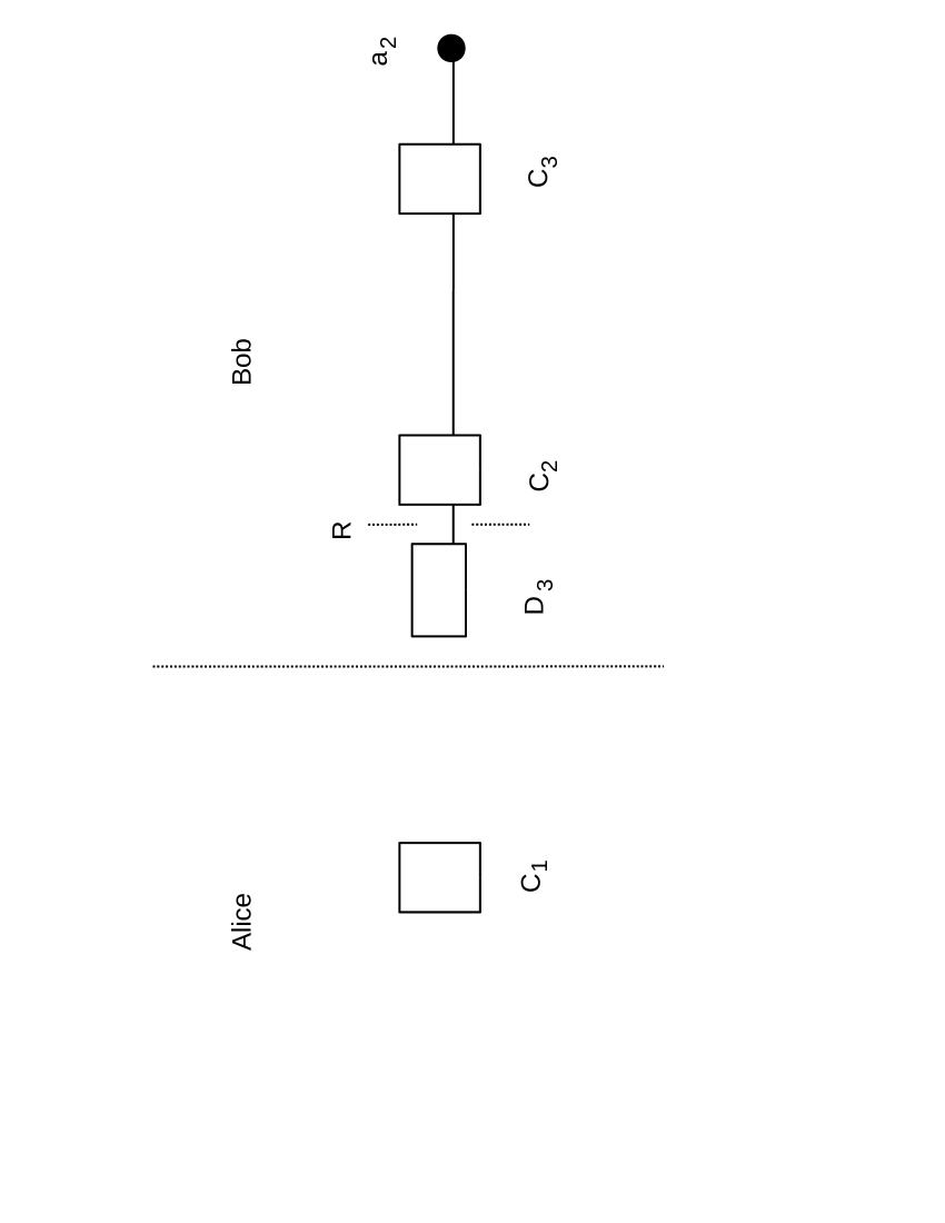
Figure 2: Set-up for Experiment-2. Alice checks directly for a photon in cavity $C_{1}$. Bob passes the atom $a_{2}$, initially in its upper level, through $C_{3}$ and $C_{2}$, before detecting it at $D_{3}$ again in its upper level. ($v_{a_{2}}=161\text{m/s}$, $k(a_{2};C_{2})=1$, $k(a_{2};C_{3})<1$).

Experiment 2.- In this case Alice checks whether the photon is present inside her cavity $C_{1}$, as in experiment 1. Bob takes his auxiliary cavity $C_{3}$ in state $|0\rangle_{C_{3}}$ and passes another atom $a_{2}$ in state $|e\rangle_{a_{2}}$ (shown in Fig. 2) through $C_{3}$ and $C_{2}$ with flight times $t_{23}$ and $t_{22}$ respectively. Bob then applies a $\frac{\pi}{2}R_{1}$ pulse on $a_{2}$, before detecting it at $D_{3}$. Now consider the case when Alice detects no photon inside her cavity $C_{1}$. The probability for this case happening is given by $\alpha_{1}^{2}(t_{11})$. Then, after Bob passes $a_{2}$ through his cavities $C_{3}$ and $C_{2}$, and applies the $\frac{\pi}{2}R_{1}$ pulse, suppose that $a_{2}$ is detected in the state $|e\rangle_{a_{2}}$. The atom $a_{2}$ was initially in the state $|e\rangle_{a_{2}}$ as well, and hence this means that in its flight it has not lost its energy by dumping any photon. Now choosing the velocity of $a_{2}$ (corresponding to the flight time $t_{22}$) through the cavity $C_{2}$ to be $v_{a_{2}}=161m/s$ and $k(a_{2};C_{2})=1$, it follows that in this case Bob’s state is given by

$$|\psi\rangle_{B}=N_{1}((-\alpha_{1}(t_{12})\alpha_{1}(t_{23})+\alpha_{2}(t_{12})\alpha_{1}(t_{23}))|1\rangle_{C_{2}}|0\rangle_{C_{3}}-(\alpha_{1}(t_{12})\alpha_{2}(t_{23})+\alpha_{2}(t_{12})\alpha_{2}(t_{23}))|0\rangle_{C_{2}}|1\rangle_{C_{3}})$$ (8)

where, $N_{1}=1/\sqrt{1-2\alpha_{2}(t_{12})\alpha_{1}(t_{12})(\alpha_{1}^{2}(t_{23})-\alpha_{2}^{2}(t_{23}))}$. Note here that with the above choice of the velocity $v_{a_{2}}$ and $k(a_{2};C_{2})$, the possibility of obtaining a two-photon state such as $|1\rangle_{C_{2}}|1\rangle_{C_{3}}$ gets ruled out (since $\alpha_{1}(t_{22})=0$ and $\alpha_{2}(t_{22})=1$). Further, let us choose $v_{a_{1}}=179\text{ m/s}$ and $k(a_{1};C_{2})=1$ (i.e., $\alpha_{1}(t_{12})=1/\sqrt{2}=\alpha_{2}(t_{12})$), such that the first term on the r.h.s. of Eq.(8) vanishes. With such a choice of the interaction parameters, it follows that Bob can find the photon in cavity $C_{3}$ only, but not in $C_{2}$. In other words, in the case when Alice detects no photon in her cavity $C_{1}$, if Bob detects a single photon, it must be in cavity $C_{3}$, and not in cavity $C_{2}$. Now, reversing this argument, if Bob detects a photon in cavity $C_{2}$, and nothing in $C_{3}$ (it follows from Eqs.(6) and (8), that such an outcome occurs with a finite probability given by $1-\alpha_{1}^{2}(t_{11})\alpha_{2}^{2}(t_{23})$), then Alice cannot detect no photons inside her cavity $C_{1}$, i.e., she must detect a single photon there, since this is the only other possible outcome.

Note here that in the above argument we have specifically chosen to describe the case when the atom is detected in the excited state $|e\rangle_{a_{2}}$. However, it needs to be mentioned that a similar argument can also be constructed in the case when the atom is detected in the ground state $|g\rangle_{a_{2}}$. The only difference between the two cases are the values of the experimental parameters required for the scheme to work out. For example, the state corresponding to Eq.(8) in the latter case would be given by $N_{1}[-\alpha_{1}(t_{23})(\alpha_{1}(t_{12})+\alpha_{2}(t_{12})|10\rangle_{C_{2}C_{3}}+\alpha_{2}(t_{23})(\alpha_{2}(t_{12})-\alpha_{1}(t_{12}))|01\rangle_{C_{2}C_{3}}]$, where $N_{1}^{2}=1/(1+2\alpha_{1}(t_{12})\alpha_{2}(t_{12})(\alpha_{1}^{2}(t_{23})-\alpha_{2}^{2}(t_{23})))$ with the probability of detection of $a_{2}$ in ground state being $1/(2N_{1}^{2})$. It follows that in this case one would require $v_{a_{1}}=146m/s$ (in stead of $179m/s$ as required in the former case) in order to ensure that the photon is found in cavity $C_{3}$ and not in $C_{2}$.

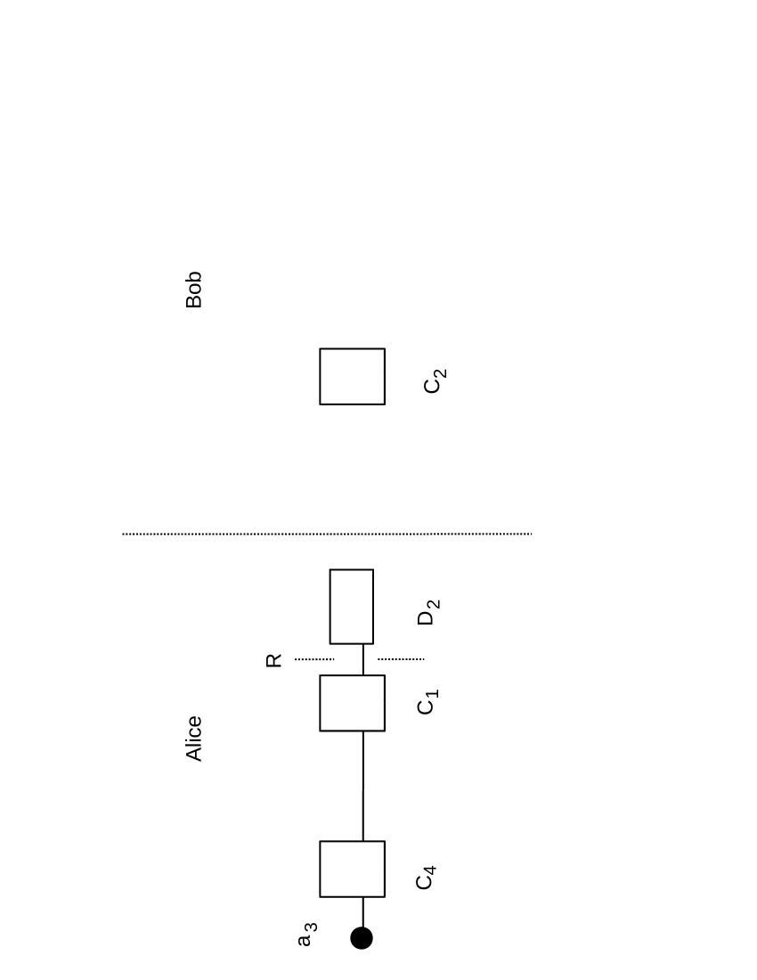
Figure 3: Set-up for Experiment-3. Bob checks directly for a photon in cavity $C_{2}$. Alice passes the atom $a_{3}$, initially in its upper level, through $C_{4}$ and $C_{1}$, before detecting it at $D_{2}$ again in its upper level. ($v_{a_{3}}=161\text{m/s}$, $k(a_{3};C_{1})=1$, $k(a_{3};C_{4})<1$).

Experiment 3.- This is similar to experiment-2, with the roles of Alice and Bob reversed. Bob checks whether the photon is present inside his cavity $C_{2}$, as in experiment 1. Alice takes her auxiliary cavity $C_{4}$ in state $|0\rangle_{C_{4}}$ and passes another atom $a_{3}$ in state $|e\rangle_{a_{3}}$ (shown in Fig. 3) through $C_{4}$ and $C_{1}$ with flight times $t_{34}$ and $t_{31}$ respectively. Alice then applies a $\frac{\pi}{2}R_{1}$ pulse on $a_{3}$, before detecting it at $D_{2}$. Now consider the case when Bob detects no photon inside his cavity $C_{2}$. Further, suppose that $a_{3}$ is detected by Alice in the state $|e\rangle_{a_{3}}$. Then, by choosing the value $v_{a_{3}}=161\text{ m/s}$ and $k(a_{3};C_{1})=1$, it follows that in this case Alice’s state is given by

$$|\psi\rangle_{A}=N_{3}((-\alpha_{1}(t_{11})\alpha_{1}(t_{12})\alpha_{1}(t_{34})+\alpha_{1}(t_{34})\alpha_{2}(t_{11}))|0\rangle_{C_{4}}|1\rangle_{C_{1}}$$

$$-(\alpha_{1}(t_{11})\alpha_{1}(t_{12})\alpha_{2}(t_{34})+\alpha_{2}(t_{34})\alpha_{2}(t_{11}))|1\rangle_{C_{4}}|0\rangle_{C_{1}})$$ (9)

with $N_{3}=1/\sqrt{\frac{\alpha_{1}^{2}(t_{11})}{2}+\alpha_{2}^{2}(t_{11})-\sqrt{2}\alpha_{1}(t_{11})\alpha_{2}(t_{11})(\alpha_{1}^{2}(t_{34})-\alpha_{2}^{2}(t_{34}))}$. Using the value of $\alpha_{1}(t_{12})=1/\sqrt{2}$ from Experiment-2, it follows that the first term on the r.h.s. of Eq.(9) vanishes when we set $v_{a_{1}}=179\text{ m/s}$ and $k(a_{1};C_{1})=0.979$, (i.e., $\alpha_{1}(t_{11})=\sqrt{2}\alpha_{2}(t_{11})$). Hence, Alice can find the photon in cavity $C_{4}$ only, but not in $C_{1}$. In other words, in the case when Bob detects no photon in his cavity $C_{2}$, if Alice detects a single photon, it must be in cavity $C_{4}$, and not in cavity $C_{1}$. Now, reversing this argument, if Alice detects a photon in cavity $C_{1}$, and nothing in $C_{4}$ (it follows from Eqs.(6) and (9), that such an outcome occurs with a finite probability given by $1-\alpha_{2}^{2}(t_{34})\alpha_{1}^{2}(t_{11})$), then Bob cannot detect no photons inside his cavity $C_{2}$, i.e., he must detect a single photon there, since this is the only other possible outcome.

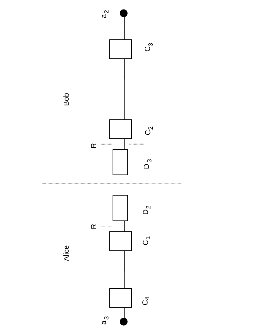
Figure 4: Set-up for Experiment-4. Alice does the same as she did in experiment-3, while Bob does the same as in experiment-2.

Experiment 4.- In this experiment (shown in Fig. 4) Alice and Bob both use there auxiliary cavities. Alice passes her atom $a_{3}$ through $C_{4}$ and $C_{1}$, and Bob passes his atom $a_{2}$ through $C_{3}$ and $C_{2}$. Further, both apply $\frac{\pi}{2}R_{1}$ pulses on their atoms which are subsequently detected in their upper states $|e\rangle_{a_{3}}$ and $|e\rangle_{a_{2}}$ respectively. One of the possibilities of this experiment is that Alice detects a photon in cavity $C_{1}$ and nothing in $C_{4}$, while Bob detects a photon in cavity $C_{2}$ and nothing in $C_{3}$, as is reflected from the following term

$$|\psi\rangle_{AB}=[-\alpha_{1}(t_{11})\alpha_{1}(t_{12})\alpha_{1}(t_{23})\alpha_{1}(t_{34})\alpha_{2}(t_{31})\alpha_{2}(t_{22})+\alpha_{1}(t_{11})\alpha_{1}(t_{12})\alpha_{1}(t_{23})\alpha_{1}(t_{34})\alpha_{2}(t_{31})$$

$$+\alpha_{2}(t_{11})\alpha_{1}(t_{23})\alpha_{1}(t_{34})\alpha_{2}(t_{22})]|1\rangle_{C_{1}}|1\rangle_{C_{2}}|0\rangle_{C_{3}}|0\rangle_{C_{4}}+......$$ (10)

in their joint state $|\psi\rangle_{AB}$. Such an outcome occurs with the probability $0.0847\alpha_{1}^{2}(t_{23})\alpha_{1}^{2}(t_{34})$. Note here that one can choose values for the parameters $k(a_{2}:C_{3})$ and $k(a_{3};C_{4})$ such that this probability is non-vanishing. The maximum probability $0.0847$ occurs for $k(a_{2}:C_{3})=k(a_{3};C_{4})=0.8$ ($\alpha_{1}(t_{23})=\alpha_{1}(t_{34})=1$).

The result of experiment-4 leads to a contradiction when combined with the other experiments, as follows. Once Alice finds a photon in cavity $C_{1}$, following the logic of experiment-3 she infers that Bob must find a photon if he were to check directly for it in his cavity $C_{2}$ without using auxiliary resources of $C_{3}$ and $a_{2}$. Similarly, on finding a photon in cavity $C_{2}$, Bob infers using the logic of experiment-2 that Alice would find a photon in $C_{1}$ if she were to check directly for it in her cavity $C_{1}$ without using auxiliary resources of $C_{4}$ and $a_{3}$. However, they both cannot be right, since it follows from the result of experiment-1 that both Alice and Bob could never detect a photon each by directly checking for it in their respective cavities $C_{1}$ and $C_{2}$ without using their auxiliary resources. The contradiction arises from the fact that the above inferences of Alice and Bob are based on the criterion of locality Hardy . The consideration of locality leads to the assumption that the probability of Bob obtaining an outcome is independent of the experiment Alice performs, and vice-versa. There is no contradiction if one does not use this assumption of locality, and hence, the conclusion follows about the nonlocality of the single photon state (6).

Concluding remarks.—

Before concluding, it is worth mentioning certain points of comparison of our proposal for testing the nonlocality of single photon states using cavities and two-level atoms, with the earlier schemes of Hardy Hardy and Dunningham and Vedral DV . Apart from the analogous nature of the argument leading to the above-mentioned contradiction with the locality assumption, the algebra of the relevant states bears formal resemblance to those used in the earlier works Hardy ; DV . This is to be expected since at the level of state preparation what we have done in the present scheme is to replace the beam-splitter and incident vacuum modes by a two-level atom passing through two intially empty cavities. There are some additional differences from the earlier schemes in the detection mechanism used in the experiments-2, 3 and 4. Here we employ auxiliary cavities and additional two-level atoms, in stead of the homodyne detection scheme. In the present scheme two-photon terms simply drop out by the choice of interaction parameters, whereas, in the scheme DV state truncation is required to ensure that the possibility of the presence of two photon states is avoided. Note that the choice of the velocities of the atoms that we have proposed in the various experiments ($v_{a_{1}}=179\text{m/s}$, and $v_{a_{2}}=161\text{m/s}=v_{a_{3}}$) fall within the thermally accessible range of velocities apr2 ; apr4 . The values for the other interaction parameter ($k\equiv\hat{{\bf d}}_{eg}.\hat{{\bf e}}({\bf r})$) that we have chosen ($k(a_{1};C_{1})=0.979$, $k(a_{1};C_{2})=k(a_{2};C_{2})=k(a_{3};C_{1})=1$, and $k(a_{2};C_{3})<1$, $k(a_{3};C_{4})<1$), should also be attainable. Further, making use of resonant interactions between atoms and cavities enables us to avoid using coherent Hardy or mixed DV states that may be difficult to create experimentally. To summarize, our proposal is based on generating atom-cavity entanglement that has already been practically operational for many years now cavexpts . Thus, our scheme should facilitate testing the nonlocality of single photons in an actual experiment free of conceptual loopholes.

Acknowledgements ASM and DH acknowledge support from the DST project no. SR/S2/PU-16/2007. DH thanks Centre for Science, Kolkata for support.

References

- (1) A. Einstein, B. Podolsky, and N. Rosen, Phys. Rev. 47, 777 (1935).
- (2) J. S. Bell, Physics 1, 195 (1964).
- (3) A. Aspect, P. Grangier, and G. Roger, Phys. Rev. Lett. 47, 460 (1981); A. Aspect, P. Grangier, and G. Roger, Phys. Rev. Lett. 49, 91 (1982); A. Aspect, J. Dalibard, and G. Roger, Phys. Rev. Lett. 49, 1804 (1982); W. Tittel, J. Brendel, H. Zbinden, N. Gisin, Phys. Rev. Lett. 81, 3563 (1998); J. W. Pan, D. Bouwmeester, M. Daniell, H. Weinfurter, A. Zeilinger, Nature 403, 515 (2000).
- (4) M. Jammer, The Philosophy of Quantum Mechanics, (Wiley-Interscience Publications, New York, 1974) p 115.
- (5) S. M. Tan, D. F. Walls, and M. J. Collett, Phys. Rev. Lett. 66, 252 (1991).
- (6) E. Santos, Phys. Rev. Lett. 68, 894 (1992); S. M. Tan, D. F. Walls, and M. J. Collett, Phys. Rev. Lett. 68, 895 (1992).
- (7) S. Basu, S. Bandyopadhyay, G. Kar and D. Home, Phys. Lett. A 279, 281 (2001); Y. Hasegawa, R. Loidl, G. Badurek, M. Baron and H. Rauch, Nature 425, 45 (2003).
- (8) S. Adhikari, A. S. Majumdar, D. Home, A. K. Pan, Europhys. Lett. 89, 10005 (2010); T. Pramanik, S. Adhikari, A. S. Majumdar, D. Home, A. K. Pan, Phys. Lett. A 374, 1121 (2010).
- (9) L. Hardy, Phys. Rev. Lett. 71, 1665 (1993).
- (10) L. Hardy, Phys. Rev. Lett. 73, 2279 (1994).
- (11) D. M. Greenberger, M. A. Horne and A. Zeilinger, Phys. Rev. Lett. 75, 2064 (1995).
- (12) D. Home and G. S. Agarwal, Phys. Lett. A 209, 1 (1995).
- (13) J. Dunningham, and V. Vedral Phys. Rev. Lett. 99, 180404 (2007).
- (14) B. Hessmo, P. Usavech, H. Heydari, G. Bjork, Phys. Rev. Lett. 92, 180401 (2004).
- (15) J. M. Raimond, M. Brune, S. Haroche Rev. Mod. Phys. 73, 565 (2001).
- (16) B.-G. Englert, M. O. Scully and H. Walther, J. Mod. Opt. 47, 2213 (2000); A. S. Majumdar and N. Nayak, Phys. Rev. A 64, 013821 (2001); A. Datta, B. Ghosh, A. S. Majumdar and N. Nayak, Europhys. Lett. 67, 934 (2004); P. Lougovski, H. Walther and E. Solano, Eur. J. Phys. D 38, 423 (2006); B. Ghosh, A. S. Majumdar, N. Nayak, Phys. Rev. A 74, 052315 (2006).
- (17) G. Rempe, F. Schmidt-Kaler and H. Walther, Phys. Rev. Lett. 64, 2783 (1990); M. Brune, S. Haroche, V. Lefevre, J. M. Raimond, and N. Zagury, Phys. Rev. Lett. 65, 976 (1990); M. O. Scully, G. M. Meyer and H. Walther, Phys. Rev. Lett. 76, 4144 (1996); A. Rauschenbeutel, G. Nogues, S. Osnaghi, P. Bertet, M. Brune, J. M. Raimond, and S. Haroche, Phys. Rev. Lett. 83, 5166 (1999); F. Cassagrande, A. Ferraro, A. Lulli, R. Bonifacio, E. Solano and H. Walther, Phys. Rev. Lett. 90, 183601 (2003); P. Maioli, T. Meunier, S. Gleyzes, A. Auffeves, G. Nogues, M. Brune, J. M. Raimond, and S. Haroche, Phys. Rev. Lett. 94, 113601 (2005).
- (18) B. Sherman, G. Kurizki, A. Kadyshevitch, Phys. Rev. Lett. 69, 1927 (1992); M. Konpka and V. Buek, Eur. Phys. J. D 10, 285 (2000); N. Vats and T. Rudolph, J. Mod. Opt. 48, 1495 (2001).
- (19) D. G. Angelakis and P. L. Knight, Eur. Phys. J. D 18, 247 (2002).