High-dimensional Bell test for a continuous variable state in phase space and its robustness to detection inefficiency

Abstract

We propose a scheme for testing high-dimensional Bell inequalities in phase space. High-dimensional Bell inequalities can be recast into the forms of a phase-space version using quasiprobability functions with the complex-valued order parameter. We investigate their violations for two-mode squeezed states while increasing the dimension of measurement outcomes, and finally show the robustness of high-dimensional tests to detection inefficiency.

I Introduction

Quantum nonlocality confirms the validity of quantum mechanics against the local-realistic theories by violations of the constraints on the correlation between local measurement outcomes. Such constraints, called Bell inequalities, were first proposed by Bell Bell64 , and to date, many versions have been proposed and investigated CHSH69 ; Collins02 ; WSon05 . Probably the best known version of Bell inequalities is Clauser, Horne, Shimony, and Holt’s (CHSH) inequality CHSH69 , which has been used for verifying nonlocal correlations in a two-dimensional Hilbert space. However, since most physical systems are composed of many particles with many degrees of freedom and thus exhibit their properties in a higher-dimensional Hilbert space, studying high-dimensional quantum correlation is essential. Recently, orbital angular momentum states of photon pairs Mair2001 and hyperentangled states Barreiro2005 have been of great interest. It has been shown that high-dimensional versions of quantum information processing offer some advantages e.g. a robust quantum key distribution Bruss2002 , superdense coding Barreiro2008 , and fast high fidelity quantum computation Vallone2008 .

Several types of high-dimensional Bell inequalities have been proposed and investigated in various ways. For example, the type proposed by Collins et al. Collins02 is in the form of a combination of joint probabilities, which we will call the CGLMP inequality throughout this paper. The violation of the CGLMP inequality was demonstrated for arbitrary high-dimensional entangled states and experimentally realized for three-dimensional systems Vaziri2002 . The type proposed by Son et al. WSon05 , which we will call the SLK inequality, is in the form of a combination of correlation functions. A generalized structure of high-dimensional Bell inequalities was formulated both in joint probability and correlation function representation where two representations are in Fourier transform relations SWLee07 .

Phase-space formalism has been used successfully for describing various quantum properties (especially for optical quantum states), since any quantum state can be perfectly characterized by quasiprobability functions such as the Wigner function, the $Q$-function, and the $P$-function Cahill69 . Bell inequalities in the forms of the CHSH inequality and the CH inequality (another version of two-dimensional Bell inequality CH74 ) were proposed by the Wigner and $Q$-functions, respectively Banaszek99 . Recently, a generalized version merging the CHSH and CH types was formulated, which provides a way of testing quantum nonlocality using quasiprobability functions with an arbitrary nonpositive order parameter (which includes the $Q$-function and the Wigner function) SWLee09 . However, so far high-dimensional quantum nonlocality has been rarely studied in phase-space formalism, in spite of a recent study WSon06 , probably because of the difficulty in discriminating multi-level outcomes efficiently.

Indeed, the inefficiency of realistic detectors is one of the biggest problems when implementing a Bell inequality test for optical quantum states. The lowest efficiency bound for observing the violation of local realism free from the detection loophole is known to be very high (e.g. about 83% for a Bell-CHSH inequality test using an entangled photon pair), and such a high efficiency is extremely difficult to achieve using current technology. It was shown that the $Q$-function permits the lowest bound efficiency for observing nonlocality in phase space SWLee09 . An entanglement witness was proposed in phase space, which enables detecting entanglement (but not nonlocality) even with significantly low detection efficiencies SWLee10 . Very recently, it was shown that high-dimensional Bell tests provide a lower bound for detection-loophole-free nonlocality tests Tamas2010 .

In this paper we present a scheme for testing high-dimensional Bell inequalities in phase-space formalism and show their robustness to detection inefficiencies. The CHSH ineq,uality can be tested in phase space Banaszek99 exploiting the fact that the Wigner function is given as an expectation of the parity measurement on photon number outcomes, i.e., $W(0)=(2/\pi)\langle(-1)^{\hat{n}}\rangle$. This is a projection of photon number statistics of a given quantum state to the two-dimensional Hilbert space with two outcomes, $+1$ and $-1$. In our approach we increase the number of outcomes to an arbitrary number $d$ by mapping the photon number into a discrete phase in polar representation, and thus, the outcomes are given as a complex variable $\langle\omega^{\hat{n}}\rangle$, where $\omega=\exp({2\pi i/d})$. The expectation value of $d$-level outcomes can be regarded as a generalized quasiprobability function with a complex order parameter. This approach has been already used in WSon06 to demonstrate the violation of the CGLMP inequality for two-mode squeezed vacuum states. In this paper, we (i) reformulate the CGLMP and SLK inequalities in the forms of generalized structure using quasiprobability functions, (ii) investigate their violations for two-mode squeezed vacuum states with different numbers of outcomes, and (iii) finally show that the CGLMP inequality can offer more robust nonlocality tests to detection inefficiency than the CHSH inequality.

This paper is organized as follows. In Sec. II we reformulate two types of high-dimensional Bell inequalities, CGLMP and SLK, in the complex variable representation. We then investigate their violations for two-mode squeezed vacuum states in Sec. III and compare their tendencies as the number of measurement outcomes $d$ increases. We also investigate the effect of detection inefficiencies on the violations of high-dimensional Bell inequalities by comparing it to the two-dimensional case. Finally, we discuss and conclude our study in Sec. IV.

II High-dimensional Bell inequalities in the complex-variable representation

In this section, we reformulate two types of high-dimensional Bell inequalities, CGLMP and SLK, in the complex-variable representation. Suppose that each observer independently chooses one of two observables, $A_{1}$ or $A_{2}$ for Alice and $B_{1}$ or $B_{2}$ for Bob with outcomes $k$ for Alice and outcomes $l$ for Bob, where $k,l\in\{0,1,...,N-1\}$. Outcomes of each observable are binned to $d$ subsets by assigning complex variables $\omega^{k}$ and $\omega^{l}$, where $\omega=\exp(2\pi i/d)$. We can define a correlation function based on complex variables and then rewrite two types of Bell inequalities in the complex-variable representation.

II.1 Correlation functions mapped to complex variable

A correlation function of two separately measured outcomes is generally given in the form

$$C=\sum^{N-1}_{k,l=0}\mu(k,l)P(A=k,B=l),$$ (1)

where $P(A=k,B=l)$ is the joint probability of Alice and Bob obtaining outcomes $k$ and $l$ and $\mu(k.l)$ is the correlation weight as a function of outcomes $k$ and $l$. We assume here that the correlation weight $\mu(k,l)$ satisfies certain conditions SWLee07 : (C1) The correlation expectation vanishes for a bipartite system with a locally unpolarized subsystem, $\sum_{k}\mu(k,l)=0,\forall l$ and $\sum_{l}\mu(k,l)=0,\forall k$. (C2) The correlation weight is unbiased over possible outcomes of each subsystem (i.e., translational symmetry within modulo $d$), $\mu(k,l)=\mu(k+\gamma,l+\gamma),\forall\gamma$. (C3) The correlation weight is uniformly distributed modulo $d$, $|\mu(k+1,l)-\mu(k,l)|=|\mu(k,l+1)-\mu(k,l)|,\forall k,l$. These are naturally required conditions for a symmetrical and locally unbiased nature assigned to the correlation functions.

A correlation weight $\omega^{k-l}$ satisfies all these conditions (though it is not a unique type), which is obtained by extending correlation functions to complex variables. Higher-order ($n$) correlations are represented by the $n$-th power of correlation weight, $\omega^{n(k-l)}$ where $n$ is a positive integer. Thus, the $n$-th order correlation function is

$$C^{(n)}=\sum_{k,l=0}^{N-1}\omega^{n(k-l)}P(A=k,B=l),$$ (2)

which shows the periodicity of $C^{(d+n)}=C^{(n)}$. Note that any Hermitian observable operator $\hat{H}$ can be associated with a unitary operator $\hat{U}$ by the simple correspondence $\hat{U}=\exp{(i\hat{H})}$. Therefore, any $N$-dimensional outcomes of $A$ and $B$ can be mapped into complex values $\omega^{k}$ and $\omega^{l}$ with a given $d$.

II.2 CGLMP inequality

We can reformulate the CGLMP inequality in complex variable representation. The CGLMP function was originally proposed as a combination of joint probabilities Collins02 and can be written in a generalized form SWLee07 :

$${\cal B}=\sum^{2}_{a,b=1}\sum_{k^{\prime},l^{\prime}=0}^{d-1}\epsilon_{ab}(k^{\prime},l^{\prime})P(\omega^{A_{a}}=\omega^{k^{\prime}},\omega^{B_{b}}=\omega^{l^{\prime}}),$$ (3)

with coefficients

$$\epsilon_{11}(k^{\prime},l^{\prime})=1-\frac{2\dot{(k^{\prime}-l^{\prime})}}{d-1},~{}~{}\epsilon_{12}(k^{\prime},l^{\prime})=1-\frac{2\dot{(l^{\prime}-k^{\prime})}}{d-1},$$

$$\epsilon_{21}(k^{\prime},l^{\prime})=-1+\frac{2\dot{(l^{\prime}-k^{\prime})}}{d-1},~{}~{}\epsilon_{22}(k^{\prime},l^{\prime})=1-\frac{2\dot{(k^{\prime}-l^{\prime})}}{d-1},$$

where the overdot implies the positive residue modulo $d$. The Bell function (3) should be bounded by $2$ in local-realistic theories. The joint probability $P(\omega^{A}=\omega^{k^{\prime}},\omega^{B}=\omega^{l^{\prime}})$ indicates the probability that the outcomes by positive residue modulo $d$ of $A$ and $B$ are equal to $k^{\prime}$ and $l^{\prime}$, respectively. This is the expectation of the projection operator $\sum^{m-1}_{p=0}|pd+k^{\prime}\rangle\langle pd+k^{\prime}|\otimes\sum^{m-1}_{q=0}|qd+l^{\prime}\rangle\langle qd+l^{\prime}|$ in $d$-dimensional Hilbert space where we assume that $N=dm$ and $m$ is an integer.

We can rewrite the CGLMP function in terms of the correlation functions (2). On the basis of the generalized formalism in SWLee07 , any Bell type inequality can be written by the sum of high-order correlation functions $C^{(n)}$ in complex space:

$${\cal B}=\sum^{2}_{ab=1}\sum^{d-1}_{n=0}f_{ab}(n)C^{(n)}_{ab},$$ (4)

where the coefficients $f_{ab}(n)$ are functions of the correlation order $n$ and the measurement configurations $a,b$. Note that it is sufficient to consider first order to $d-1$-order correlation functions due to the periodicity $C^{(d+n)}=C^{(n)}$. The zeroth-order correlation has no meaning as it simply shifts the value of ${\cal B}$ by a constant value and is thus here chosen to vanish, i.e., $\sum_{a,b}f_{ab}(0)=0$. The CGLMP inequality can then be recast into

$${\cal B}_{\mathrm{CGLMP}} = \frac{2}{d-1}\sum_{n=1}^{d-1}\frac{1}{1-\omega^{-n}}\biggl{[}C^{(n)}_{11}-\omega^{-n}C^{(n)}_{12}$$ (5)

$$~{}~{}~{}~{}~{}~{}~{}~{}~{}~{}~{}~{}~{}~{}~{}-C^{(n)}_{21}+C^{(n)}_{22}\biggr{]}\leq 2,$$

where $C^{(n)}_{ab}=\sum^{d-1}_{k^{\prime},l^{\prime}=0}\omega^{n(k^{\prime}-l^{\prime})}P(\omega^{A_{a}}=\omega^{k^{\prime}},\omega^{B_{b}}=\omega^{l^{\prime}})$ is the $n$-th order correlation function. Note that the expectation value of the Bell function in Eq. (5) is always real even though it is represented by complex variables. The correlation function can be obtained as an expectation value of the correlation operator,

$$\hat{C}^{(n)}_{ab} = \sum^{d-1}_{k^{\prime},l^{\prime}=0}\omega^{n(k^{\prime}-l^{\prime})}\sum^{m-1}_{p=0}|pd+k^{\prime}\rangle_{a}\langle pd+k^{\prime}|$$ (6)

$$~{}~{}~{}~{}~{}~{}~{}~{}~{}~{}~{}~{}~{}\otimes\sum^{m-1}_{q=0}|qd+l^{\prime}\rangle_{b}\langle qd+l^{\prime}|,$$

$$= \sum^{N-1}_{k,l=0}\omega^{n(k-l)}|k\rangle_{a}\langle k|\otimes|l\rangle_{b}\langle l|,$$

where each local measurement basis, denoted by the notation $a$, $b$ can be differentiated by unitary operation in $d$-dimensional Hilbert space. Note that when $d=2$, Eq. (5) becomes the CHSH inequality $C_{11}+C_{12}-C_{21}+C_{21}\leq 2$ where $\hat{C}_{ab}=\sum^{N-1}_{k,l=0}(-1)^{k+l}|k\rangle_{a}\langle k|\otimes|l\rangle_{b}\langle l|$.

II.3 SLK inequality

We then consider the SLK inequality in the complex-variable representation. On the basis of the generalized structure in Eq. (4), we can obtain the SLK function in the form of Eq. (3) with the coefficients SWLee07

$$\epsilon_{11}(k^{\prime},l^{\prime})=S(k^{\prime}-l^{\prime}+\frac{1}{4}),~{}~{}\epsilon_{12}(k^{\prime},l^{\prime})=S(k^{\prime}-l^{\prime}-\frac{1}{4}),$$

$$\epsilon_{21}(k^{\prime},l^{\prime})=S(k^{\prime}-l^{\prime}+\frac{3}{4}),~{}~{}\epsilon_{22}(k^{\prime},l^{\prime})=S(k^{\prime}-l^{\prime}+\frac{1}{4}),$$

where $S(x\neq 0)=(1/4)(\cot{\frac{\pi x}{d}}\sin{2\pi x}-\cos{2\pi x}-1)$ and $S(x=0)=(d-1)/2$. The local-realistic bound of the SLK function is given as a function of the number of outcomes $d$ by $\frac{1}{4}(3\cot{\frac{\pi}{4d}}-\cot{\frac{3\pi}{4d}})-1$. In order to compare it to the CGLMP inequality with a fixed local-realistic bound $2$, we recast the original form of the SLK inequality into

$${\cal B}_{\mathrm{SLK}} = \frac{1}{R(d)}\sum_{n=1}^{d-1}\biggl{[}(\omega^{\frac{n}{4}}+\omega^{\frac{n-d}{4}})C^{(n)}_{11}$$ (7)

$$+(\omega^{-\frac{n}{4}}+\omega^{-\frac{n-d}{4}})C^{(n)}_{12}+(\omega^{\frac{3n}{4}}+\omega^{\frac{3(n-d)}{4}})C^{(n)}_{21}$$

$$~{}~{}~{}~{}~{}~{}~{}~{}~{}~{}~{}~{}~{}~{}~{}~{}+(\omega^{\frac{n}{4}}+\omega^{\frac{n-d}{4}})C^{(n)}_{22}\biggr{]}\leq 2,$$

where $R(d)=3\cot{\frac{\pi}{4d}}-\cot{\frac{3\pi}{4d}}-4$. Note that the expectation value of Eq. (7) is always real and when $d=2$ it becomes equivalent to the CHSH inequality.

Two high-dimensional Bell inequalities in the complex-variable representation given in Eqs. (5) and (7) can be effectively used for testing arbitrary $N$-dimensional quantum states by arbitrary $d$-dimensional measurement. If we consider the case $N=\infty$, we can perform high-dimensional Bell tests for continuous-variable quantum states, as we will show in the following section.

III Violations of high-dimensional Bell inequalities by a continuous variable state

In this section, we investigate violations of two types of high-dimensional Bell inequalities, CGLMP and SLK, for continuous variable entangled states. We consider here the two-mode squeezed vacuum states (TMSSs)

$$|\Psi\rangle_{\mathrm{TMSS}}=\sum_{j=0}^{\infty}\frac{\tanh^{j}{r}}{\cosh{r}}|j,j\rangle,$$ (8)

where $r>0$ is the squeezing parameter and $|j\rangle$ is the number state of each mode. This can be realized by non degenerate optical parametric amplifiers Reid88 , and highly entangled photon pairs can be generated for testing Bell inequalities zhang07 . Such states are well suited to Bell inequality tests since entangled photon pairs can be generated and distributed over long distances Weihs98 ; Tittel98 .

III.1 Bell tests by reconstructing quasiprobability functions

Let us consider high-dimensional Bell tests by reconstructing quasiprobability functions. An entangled state generated from a source of correlated photons is distributed to two spatially separated parties called Alice and Bob. Each party performs a local measurement by counting photon numbers. The bases of each local measurement are differentiated by the displacement operation $\hat{D}(\alpha)$ for Alice and $\hat{D}(\beta)$ for Bob where $\alpha$ and $\beta$ are complex variables associated with points in phase space Cahill69 . If we bin the measured photon numbers alternatively into two-dimensional outcomes ($+1$ and $-1$), the expectation value of local measurement is given as a Wigner function at the point displaced $\alpha$ (or $\beta$) in phase space, i.e., $W(\alpha)=(2/\pi)\langle(-1)^{\hat{n}(\alpha)}\rangle$, where $\hat{n}(\alpha)=\hat{D}(\alpha)\hat{n}\hat{D}(-\alpha)$ is a displaced number operator. A detail experimental setup for reconstructing quasiprobability functions by photon counting is given in Banaszek96 .

For high-dimensional outcomes, we bin the counted photon numbers $k$ for Alice and $l$ for Bob into arbitrary $d$-dimensional outcomes by assigning complex variables $\omega^{k}$ and $\omega^{l}$, respectively. Therefore, the local measurement operator for Alice is given by

$$\hat{A}(\alpha)=\sum^{\infty}_{k=0}\omega^{k}\hat{D}(\alpha)|k\rangle\langle k|\hat{D}(-\alpha)\equiv\omega^{\hat{k}(\alpha)},$$ (9)

and likewise for Bob $\hat{B}(\beta)\equiv\omega^{\hat{l}(\beta)}$. The $n$th-order correlation function is then given by

$$C^{(n)}_{\alpha\beta} = \langle\hat{A}(\alpha)^{n}\hat{B}^{{\dagger}n}(\beta)\rangle$$ (10)

$$= \sum_{k,l=0}^{\infty}\omega^{n(k-l)}P_{k,l}(\alpha,\beta),$$

where $P_{k,l}(\alpha,\beta)$ is the joint probability of counting $k$ and $l$ photons at the local measurement setup of two modes displaced by $\alpha$ and $\beta$, respectively. We can rewrite the correlation function in Eq. (10) as

$$C^{(n)}=\sum^{\infty}_{k,l=0}\biggl{(}\frac{s_{n}+1}{s_{n}-1}\biggr{)}^{k-l}P_{k,l}(\alpha,\beta),$$ (11)

where $s_{n}\equiv-i\cot(n\pi/d)$. This is proportional to the two-mode $s$-parameterized quasiprobability function $W(\alpha,\beta;s)$ if we extend the parameter $s$ from a real to a complex variable. The $s$-parameterized quasiprobability function is defined as Cahill69 ; Moya93

$$W(\alpha;s)=\frac{2}{\pi(1-s)}\left\langle\left(\frac{s+1}{s-1}\right)^{\hat{n}(\alpha)}\right\rangle,$$ (12)

where $\hat{n}(\alpha)$ is a number operator displaced by a complex variable $\alpha$ in phase space. It becomes the $P$-function, the Wigner-function, and the $Q$-function when setting $s=1,0,-1$ Moya93 , respectively. Then the correlation function is written by a two-mode quasiprobability function as

$$C^{(n)}_{\alpha\beta} = \frac{\pi^{2}(1-s_{n}^{2})}{4}W(\alpha,\beta;s_{n}).$$ (13)

We define quasiprobability functions of, e.g., the two-mode squeezed vacuum states given in Eq. (8) with complex variable order parameter as follows. The characteristic function for two-mode squeezed vacuum states is defined using a complex order parameter $s_{n}$ by

$$\chi(\xi,\eta;s_{n}) = {}_{\mathrm{TMSS}}\langle\Psi|\hat{D}(\xi)\otimes\hat{D}(\eta)|\Psi\rangle_{\mathrm{TMSS}}$$

$$~{}~{}~{}~{}~{}~{}~{}~{}~{}~{}~{}~{}\times\exp(s_{n}|\xi|^{2}+s_{n}^{*}|\eta|^{2}/2)$$

$$= \exp\biggl{[}-\frac{1}{2}\{|\xi|^{2}(\cosh{2r}-s_{n})$$

$$+|\eta|^{2}(\cosh{2r}-s_{n}^{*})+(\xi\eta+\xi^{*}\eta^{*})\sinh{2r}\}\biggr{]}.$$

The corresponding quasiprobability functions can be obtained by

$$W(\alpha,\beta;s_{n}) = \frac{1}{\pi^{4}}\int^{\infty}_{-\infty}d^{2}\xi d^{2}\eta~{}\chi(\xi,\eta;s_{n})$$

$$~{}~{}~{}~{}~{}~{}\times\exp(\alpha\xi^{*}-\alpha^{*}\xi)\exp(\beta\eta^{*}-\beta^{*}\eta)$$

$$= \frac{4}{\pi^{2}(1-s_{n}^{2})}\exp\biggl{[}-\frac{2}{1-s_{n}^{2}}\{|\alpha|^{2}A^{*}$$

$$~{}~{}~{}~{}~{}~{}+|\beta|^{2}A+(\alpha\beta+\alpha^{*}\beta^{*})\sinh{2r}\}\biggr{]},$$

where $A=\cosh{2r}-s_{n}$. Therefore, from the Eqs. (11), (12), and (III.1), we obtain the correlation function for two-mode squeezed vacuum states as

$$C^{(n)}_{\alpha\beta}=\exp\biggl{[}-2\frac{|\alpha|^{2}A^{*}+|\beta|^{2}A+(\alpha\beta+\alpha^{*}\beta^{*})\sinh{2r}}{1-s_{n}^{2}}\biggr{]}.$$ (16)

Now we can rewrite two types of high-dimensional Bell inequalities in terms of quasiprobability functions; that is the correlation functions of CGLMP given in Eq. (5) and SLK in Eq. (7) can be replaced with quasiprobability functions using Eq. (13). Note that for two-dimensional outcomes $d=2$, the correlation function is proportional to the two-mode Wigner function,

$$C_{\alpha\beta}=\sum^{\infty}_{k=0}(-1)^{k-l}P_{k,l}(\alpha,\beta)=\frac{\pi^{2}}{4}W(\alpha,\beta),$$ (17)

and in this case both, CGLMP and SLK, become equivalent with the type proposed in Banaszek99 in the form of the CHSH Bell inequality.

On the basis of this formalism we will investigate violations of high-dimensional Bell inequalities, CGLMP and SLK, for any quantum state that can be represented by the quasiprobability functions.

III.2 Violations of Bell inequalities

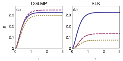
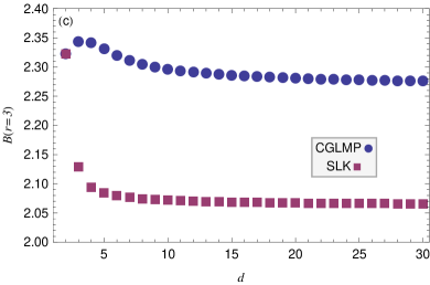
Figure 1: (Color online) Violations of the (a) CGLMP and (b) SLK inequalities for two-mode squeezed vacuum states with varying squeezing rate $r$ when $d=2$ (solid line), $d=3$ (dashed line) and $d=10$ (dotted line). (c) The expectation values of CGLMP and SLK are compared while increasing the number of outcomes $d$ for a two-mode squeezed vacuum state ($r=3$).

We investigate violations of two types of Bell inequalities, CGLMP and SLK, for two-mode squeezed vacuum states by properly choosing local measurements $\alpha$, $\alpha^{\prime}$, $\beta$ ,and $\beta^{\prime}$. The maximal expectation values of the CGLMP and SLK functions for different numbers of outcomes $d$ are plotted in Figs. 1(a) and 1(b), respectively, against the squeezing rate $r$. The expectation values of both types exceed the local-realistic bound $2$ for any $r$ and increase up to maximum as $r$ increases. However, the degrees of violation of the two types show different tendencies depending on the number of outcomes $d$ as shown in Fig. 1(c).

For CGLMP inequalities, the degree of violation reaches a maximum when $d=3$ and decreases as $d$ increases. Tests of the CGLMP inequality for $d=3$, $d=4$, and $d=5$ exhibit stronger violations than that of the CHSH inequality in agreement with the results in Ref. WSon06 . This is an advantage offered by the CGLMP inequality tests over the CHSH inequality test. For $d>5$, the degree of violation is lower than that of a two-dimensional test. Nevertheless, the expectation value does not decrease quickly so one can still verify strong violations of the local realism in high-dimensional correlations. The reason that the change in maximal expectation values with increasing $d$ does not show a monotonous tendency is because possible operations for local measurements are restricted by displacement operations in phase space instead of the full SU($d$) transformation, as pointed out in WSon06 .

On the other hand, the SLK inequalities show different tendencies. As demonstrated in Figs. 1(b) and 1(c), the degree of violation decreases as $d$ increases, in contrast to the CGLMP inequality, so it exhibits strongest violations when $d=2$. Note that when $d=2$, both CGLMP and SLK types are equivalent with the CHSH inequality and their violations by two-mode squeezed vacuum states are the same as the results obtained in Jeong03 .

III.3 Effects of detection inefficiency

In a realistic experimental setup, noise effects occur during the measurement process, such as photon losses and dark counts. In general, the photon number distribution measured by inefficient detectors $\hat{P}_{m}(\eta)$ can be modeled by the generalized Bernoulli transformation from the real number distribution $|k\rangle\langle k|$ Leonhardt-1997 :

$$\hat{P}_{m}(\eta)=\sum^{\infty}_{k=m}\binom{k}{m}(1-\eta)^{k-m}\eta^{m}|k\rangle\langle k|,$$ (18)

where $\eta$ is the overall detection efficiency and $\sum^{\infty}_{m=0}\hat{P}_{m}(\eta)=\openone$. We shall not consider dark counts here as those are relatively minor when the detection efficiency is low. It is known that dark count rates can be suppressed when low-efficiency detectors are used: Highly efficient detectors have relatively high dark count rates, while less efficient detectors have very low dark count rates Takeuchi99 .

The realistic local measurement operator for Alice with detection efficiency $\eta_{A}$ is given by

$$\hat{A}(\alpha,\eta_{A}) = \sum^{\infty}_{m=0}\omega^{m}\hat{D}(\alpha)\hat{P}_{m}(\eta)\hat{D}(-\alpha)$$ (19)

$$= \sum^{\infty}_{k=0}(1-\eta_{A}+\eta_{A}\omega)^{k}\hat{D}(\alpha)|k\rangle\langle k|\hat{D}(-\alpha)$$

$$= (1-\eta_{A}+\eta_{A}\omega)^{\hat{k}(\alpha)},$$

and likewise for Bob $\hat{B}(\beta,\eta_{B})=(1-\eta_{B}+\eta_{B}\omega)^{\hat{l}(\beta)}$.

The correlation function between Alice and Bob for two mode squeezed states is written by

$$C^{(n)}_{\alpha\beta}(\eta_{A},\eta_{B})=\frac{S(\eta_{A},\eta_{B})}{T(\eta_{A},\eta_{B})}\exp\biggl{[}-\frac{2}{T(\eta_{A},\%eta_{B})}\{|\alpha|^{2}R^{*}(\eta_{B})$$

$$+|\beta|^{2}R(\eta_{A})+(\alpha\beta+\alpha^{*}\beta^{*})\sinh{2r}\}\biggr{]},~{}~{}$$ (20)

where

$$R(\eta)=\cosh{2r}-1+\frac{1}{\eta}+\frac{i}{\eta}\cot\frac{n\pi}{d},$$

$$S(\eta_{A},\eta_{B})=\frac{1}{\eta_{A}\eta_{B}}(1+\cot^{2}\frac{n\pi}{d}),$$

$$T(\eta_{A},\eta_{B})=R(\eta_{A})R^{*}(\eta_{B})-\sinh^{2}{2r},$$

which becomes equivalent to Eq. (16) when $\eta_{A}=\eta_{B}=1$. The expectation values of CGLMP and SLK in the presence of detection inefficiency are then obtained by applying Eq. (III.3) to Eqs. (5) and (7), respectively. Since violations of the SLK inequality become weaker as $d$ increases, even in the case of perfect efficiency shown in Sec. III.2, we here consider only the CGLMP inequality.

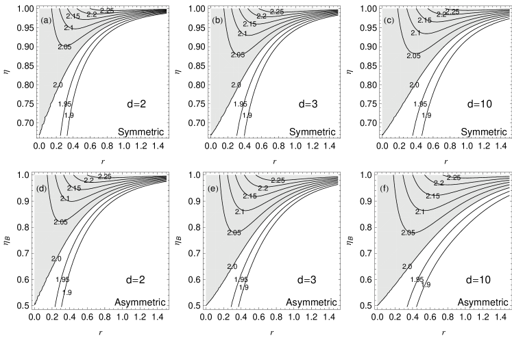
Figure 2: Expectation values of the CGLMP tests for two-mode squeezed vacuum states in symmetric cases($\eta_{A}=\eta_{B}=\eta$) for (a) $d=2$, (b) $d=3$, and (c) $d=10$, and asymmetric cases($\eta_{A}=1$) for (d) $d=2$, (e) $d=3$, and (f) $d=10$. The shaded regions indicate the violations of the CGLMP inequalities in the range of the detection efficiency $\eta$ and the squeezing rate $r$.

Let us first consider the symmetric case when the detector efficiencies of Alice and Bob are the same $\eta_{A}=\eta_{B}=\eta$. Figures 2(a), 2(b) and 2(c) show violations of the CGLMP inequality when $d=2,3$ and $10$, respectively, in the range of efficiency $\eta$ and squeezing rate $r$. It is shown that high-dimensional tests can exhibit stronger violations than that for $d=2$ in some regions of $\eta$ and $r$. Furthermore, it is noticeable that the bound efficiency for observing quantum nonlocality becomes lower as $d$ increases for a given $r>0$. For example, for a two-mode squeezed vacuum state $r=0.3$ and a detection efficiency $\eta=0.8$, one can observe quantum nonlocality when testing the CGLMP inequality with $d=10$, while one can not observe it when testing the CHSH inequality ($d=2$). We note that the bound efficiency for any $d$ is down to $\eta=0.667$ as $r$ decreases to zero, which interestingly is the Eberhard limit, i.e., the lowest bound efficiency for the CHSH Bell test Eberhard1993 . This is because for slightly squeezed states the first two levels of number basis are dominant, so the CGLMP Bell test becomes nearly equivalent to the two-dimensional test. It is also notable that for any $d$ the efficiency bound becomes higher as the squeezing rate $r$ increases, and thus, the violation for the Einstein-Podolsky-Rosen (EPR) state ($r=\infty$) is observed only when $\eta=1$. This may be because the number counting with a displacement operation is not an optimal local measurement for testing nonlocality with the EPR state, as pointed out in Ref. SWLEE09-2 .

Let us also consider an asymmetric case when $\eta_{A}=1$ and thus the effects of inefficiency are characterized only by $\eta_{B}$. This can be realized by an atom-photon entanglement since the atom is measured with an efficiency close to 1 Cabello2007 ; Brunner2007 . Figures 2(d), 2(e) and 2(f) show the violation regions of the CGLMP inequality when $d=2,3,$ and $10$, respectively, in the range of $\eta_{B}$ and $r$. Similarly to the symmetric cases, high-dimensional tests of the CGLMP inequality are shown to be more robust to detection inefficiency than the CHSH test for a given $r>0$. We note that the bound efficiency for any $d$ is down to $\eta=0.5$ as $r$ decreases to zero, which is equivalent to the lowest limit for the CHSH Bell test on atom-photon systems Cabello2007 .

It is shown that the CGLMP inequality offers a more robust nonlocality test to detection inefficiency than the CHSH inequality when using continuous-variable states. Therefore, a high-dimensional approach may provide an advantageous way of closing the detection loophole problem for quantum nonlocality tests, which is in agreement with the work in Ref. Tamas2010 .

IV Discussion and Conclusions

The complex variable representation of correlation functions can be efficiently used for testing high-dimensional quantum nonlocality. Two types of high-dimensional Bell inequalities given in Eqs. (5) and (7) are applicable in any case of complex-valued measurement. For example, as we have shown in this paper, it can be extended to continuous variables by virtue of the phase space formalism. The correlation function is then given as a quasiprobability function with a complex order parameter, which can be reconstructed by photon number counting.

We investigate the effect of detection inefficiency on the violation of high-dimensional Bell inequalities when the system is given as a pure two-mode squeezed state, while previous works have studied the effect of system noise Collins02 ; Acin2002 . Similar to the case of system noise, violations of the CGLMP inequality ($d>2$) are shown to be more robust to detection inefficiency than that of the CHSH inequality ($d=2$). In addition, the bound efficiency for demonstrating quantum nonlocality becomes lower as the dimension increases for two-mode squeezed vacuum states with a given $r>0$. This may provide a useful insight for closing the detection loophole problem in a nonlocality test with continuous-variable states. The work in Ref. SWLee09 , which shows that the $Q$-function allows more robust Bell tests to detection inefficiency than the Wigner function, can be understood relevantly since the $Q$-function can be regarded as an expectation value of high-dimensional measurements. Note that the $Q$-function is a smoothed Wigner function where the smoothing effect is modeled as a split of outcomes of parity measurements (i.e., $+1$ and $-1$) to higher-dimensional outcomes.

For an experimental realization of the proposed scheme, there exists an obstacle to overcome: the low efficiency of realistic photon-counting detectors. As an alternative method, one may consider a highly efficient homodyne tomography Vogel1989 . However, for a valid quantum nonlocality test, it is required that the quantities measured by the detectors should satisfy the local-realistic conditions assumed when deriving the Bell inequality. Note that the local-realistic bounds in Eqs. (5) and (7) are given as a maximal expectation value of a combination of photon number correlations. Alternatively, an atom-field interaction in a cavity can be considered for a high-dimensional measurement Bertet02 , but it is feasible only when the measurement dimension $d$ is a power of 2. Therefore, the realization of the proposed nonlocality test is expected with the progress of photon detection technologies Divochiy2008 .

In summary, we have proposed a scheme for testing high-dimensional Bell inequalities in phase space and investigated the effect of detection inefficiency. First, two types of high-dimensional Bell inequalities, CGLMP and SLK, are recast into a structure composed of complex-variable correlation functions. The correlation functions were shown to be proportional to the quasiprobability function with an order parameter associated with the number of outcomes, which can be reconstructed by photon number counting. On the basis of the proposed scheme, we demonstrated violations of two types of high-dimensional Bell inequalities, CGLMP and SLK, for two-mode squeezed vacuum states and compared their violations for different numbers of outcomes. For the case of two-level outcomes, violations of both types are equivalent to that of the CHSH inequality. For some cases with more than two levels of outcomes the CGLMP inequality exhibits stronger violations than the CHSH inequality, while violation of the SLK inequality tends to decrease as the number of outcomes increases. Finally, we have shown that the CGLMP inequality can offer a more robust nonlocality test to detection inefficiency than the CHSH inequality. We expect an experimental realization of high-dimensional Bell tests on continuous-variable states based on our scheme. An important next step will be to increase the number of local measurement settings, which could lower the bound efficiency further Tamas2010 ; Brunner2007 .

- (1) J. S. Bell, Physics (Long Island City, N.Y.) 1, 195 (1964).
- (2) J. F. Clauser, M. A. Horne, A. Shimony, and R. A. Holt, Phys. Rev. Lett. 23, 880 (1969).
- (3) D. Collins, N. Gisin, N. Linden, S. Massar, and S. Popescu, Phys. Rev. Lett. 88, 040404 (2002).
- (4) W. Son, J. Lee, and M. S. Kim, Phys. Rev. Lett. 96, 060406 (2006).
- (5) A. Mair, A. Vaziri, G. Weihs, and A. Zeilinger, Nature (London) 412, 313 (2001).
- (6) J. T. Barreiro, N. K. Langford, N. A. Peters, and P. G. Kwiat, Phys. Rev. Lett. 95, 260501 (2005).
- (7) D. Bruß, and C. Macchiavello, Phys. Rev. Lett. 88, 127901 (2002).
- (8) J. T. Barreiro, T.-C. Wei, and P. G. Kwiat, Nat. Phys. 4, 282 (2008).
- (9) G. Vallone, E. Pomarico, F. De Martini, and P. Mataloni, Phys. Rev. Lett. 100, 160502 (2008).
- (10) A. Vaziri, G. Weihs, and A. Zeilinger, Phys. Rev. Lett. 89 240401(2002).
- (11) S.-W. Lee, Y. W. Cheong, and J. Lee, Phys. Rev. A76, 032108 (2007).
- (12) K. E. Cahill, and R. J. Glauber, Phys. Rev. 177, 1857 (1969); Phys. Rev. 177, 1882 (1969).
- (13) J. F. Clauser, and M. A. Horne, Phys. Rev. D10, 526 (1974).
- (14) K. Banaszek, and K. Wodkiewicz, Phys. Rev. A58, 4345 (1998); Phys. Rev. Lett. 82, 2009 (1999); Acta Phys. Slov. 49, 491 (1999).
- (15) S.-W. Lee, H. Jeong, and D. Jaksch, Phys. Rev. A80, 022104 (2009).
- (16) W. Son, Č. Brukner, and M. S. Kim, Phys. Rev. Lett. 97, 110401 (2006).
- (17) S.-W. Lee, H. Jeong, and D. Jaksch, Phys. Rev. A81, 012302 (2010).
- (18) T. Vértesi, S. Pironio, and N. Brunner, Phys. Rev. Lett. 104, 060401 (2010).
- (19) M. D. Reid and P. D. Drummond, Phys. Rev. Lett. 60, 2731 (1988).
- (20) L. Zhang, A. B. U’ren, R. Erdmann, K. A. O’Donnell, C. Silberhorn, K. Banaszek, and I. A. Walmsley, J. Mod. Opt. 54, 707 (2007).
- (21) G. Weihs, T. Jennewein, C. Simon, H. Weinfurter, and A. Zeilinger, Phys. Rev. Lett. 81, 5039 (1998).
- (22) W. Tittel, J. Brendel, B. Gisin, T. Herzog, H. Zbinden, and N. Gisin, Phys. Rev. A57, 3229 (1998).
- (23) K. Banaszek, and K. Wodkiewicz, Phys. Rev. Lett. 76, 4344 (1996);
- (24) H. Moya-Cessa, and P. L. Knight, Phys. Rev. A48, 2479 (1993).
- (25) H. Jeong, W. Son, M. S. Kim, D. Ahn, and Č. Brukner, Phys. Rev. A67, 012106 (2003).
- (26) U. Leonhardt, Measuring the Quantum State of Light, (Cambridge University Press, Cambridge, 1997).
- (27) S. Takeuchi, J. Kim, Y. Yamamoto, and H. Hogue, Appl. Phys. Lett. 74, 1063 (1999).
- (28) P. H. Eberhard, Phys. Rev. A47, R747 (1993).
- (29) S.-W. Lee, and D. Jaksch, Phys. Rev. A80, 010103(R) (2009).
- (30) A. Cabello, and J.-Å. Larsson, Phys. Rev. Lett. 98, 220402 (2007).
- (31) N. Brunner, N. Gisin, V. Scarani, and C. Simon, Phys. Rev. Lett. 98, 220403 (2007).
- (32) A. Acin, T. Durt, N. Gisin, and J. I. Latorre, Phys. Rev. A65, 052325 (2002).
- (33) K. Vogel, and H. Risken, Phys. Rev. A40, 2847 (1989); D. T. Smithey, M. Beck, M. G. Raymer, and A. Faridani, Phys. Rev. Lett. 70, 1244 (1993).
- (34) P. Bertet, A. Auffeves, P. Maioli, S. Osnaghi, T. Meunier, M. Brune, J. M. Raimond, and S. Haroche, Phys. Rev. Lett. 89, 200402 (2002).
- (35) A. Divochiy et al., Nat. Photonics 2, 302 (2008); M. Avenhaus, H. B. Coldenstrodt-Ronge, K. Laiho, W. Mauerer, I. A. Walmsley, and C. Silberhorn, Phys. Rev. Lett. 101, 053601 (2008).