THE CMS EXPERIMENT: STATUS AND FIRST RESULTS

After nearly two decades of design, construction and commissioning, the CMS detector was operated with colliding LHC proton beams for the first time in November 2009. Collision data were recorded at centre-of-mass energies of 0.9 and 2.36 TeV, and analyzed with a fast turn-around time by the CMS collaboration. In this talk I will present a selection of commissioning results and striking first physics resonances observed. Then I will discuss the analysis of the transverse momentum and rapidity distribution of charged hadrons, which led to the first CMS physics publication. The excellent performance of the CMS detector and agreement with predictions from simulation are impressive for a collider detector at startup and show a great potential for discovery physics in the upcoming LHC run.

1 Introduction

The CMS experiment $\!{}^{{\bf?}}$ recorded the first LHC $\!{}^{{\bf?}}$ proton-proton collisions on Monday the 23^rd of November, 2009. In the weeks that followed, CMS collected approximately 350 thousand collision events at an energy of $\sqrt{s}$=0.9 TeV and 20 thousand events at $\sqrt{s}$=2.36 TeV with good detector conditions and the magnet switched on at the nominal value of 3.8 T. This corresponds to about 10 $\mu$b^-1 of integrated luminosity, close to 85% of the collisions delivered by the LHC.

The recorded data sample is still many orders of magnitude too small to do the physics studies for which CMS was designed. However, it is sufficient to assess the general quality and the proper functioning of the detector, the algorithms and the modeling of the detector response in the simulation. This is a crucial step in the preparation of the experiment for physics.

Section 2 briefly presents the status of CMS at startup, followed by a summary of the first physics performance results in Sections 3 to 6. These performance results formed the basis for a timely publication of the first physics measurement with collision data, one month before this conference $\!{}^{{\bf?}}$, as discussed in Section 7. This is followed by the conclusions in Section 8.

2 CMS Status at Startup

In the three years preceding the first LHC proton-proton collisions, CMS recorded and analysed more than a billion events with muons from various sources. Three cosmic ray runs in 2006, 2008 and 2009 recorded about 300 million cosmic ray muon events each. Over a million beam halo muons were recorded during LHC commissioning in 2008 and 2009, as well as more than a thousand so-called beam-splash events. These beam-splash events occur when LHC intentionally dumps a single bunch of the beam on a collimator about 150 m upstream from CMS, leading to a flood of muons traveling through the detector simultaneously.

Detailed analysis of these events resulted in crucial improvements in the alignment of the detector, modeling of the magnetic field, understanding of the response of different subdetectors to muons, calibration, noise characteristics and synchronization. The results of these studies are described in 23 performance papers $\!{}^{{\bf?}}$, submitted by CMS just before the start of collisions in 2009. The papers have been accepted by JINST and are expected to appear in a single volume of the journal, soon after this conference.

The detector simulation that was thus tested and validated before collisions was used without further adjustments in the first CMS physics paper and for all other results presented in this report. The only parameter that had to be adapted was the longitudinal distribution of the primary collision vertices, which was tuned to match the LHC operating conditions.

3 The first Physics Resonance in Collisions

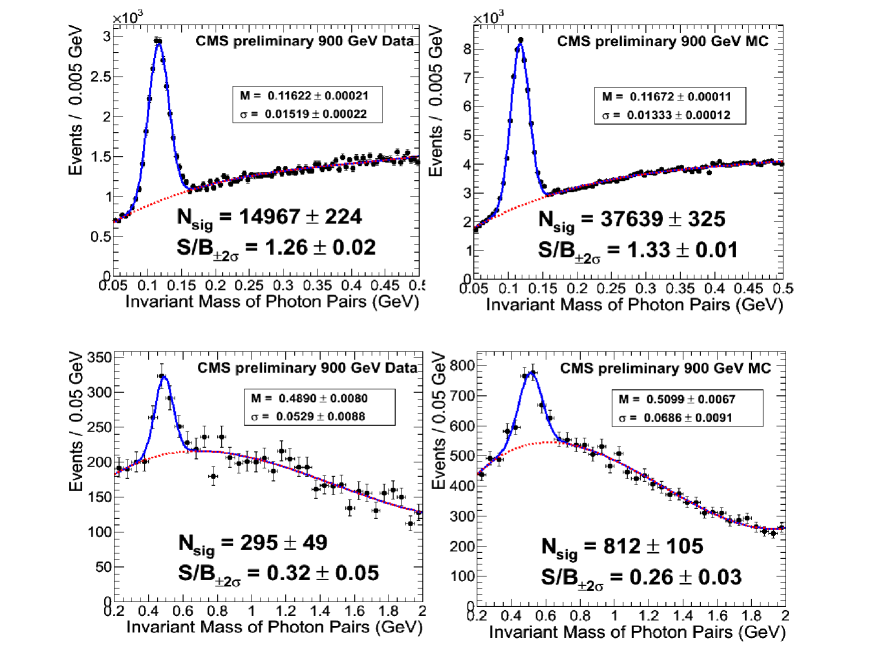
Figure 1: Uncorrected photon-pair invariant mass peaks in data (left) and simulation (right) in the region around the mass of the $\pi^{0}$ (top) and $\eta$ (bottom) resonances.

The first physics resonance observed in collision data was the di-photon invariant mass from the decay of neutral pions $\pi^{0}\rightarrow\gamma\gamma$, visible even after the first run with 191 recorded events when the experimental magnets were still switched off. The peak, together with a dedicated simulated sample (with magnetic field off) was ready and approved for public presentation within three days after the first collisions. Updated versions of the $\pi^{0}$ di-photon invariant mass plots $\!{}^{{\bf?}}$, with more data and simulated events, are shown in Fig. 1(top). For this plot only photon candidates in the barrel ($|\eta|<$1.479) are used, requiring basic shower shape cuts, a transverse photon energy $E_{\rm T}$ above 300 MeV, and the transverse momentum $p_{\rm T}$ of the reconstructed $\pi^{0}$ above 900 MeV. Similarly, the eta resonance $\eta\rightarrow\gamma\gamma$ is shown for data and simulation in Fig. 1(bottom). In this case a photon $E_{\rm T}>$ 400 MeV and $\eta$ $p_{\rm T}>$ 2 GeV was required. The masses shown are based on the measured photon energies without corrections for shower containment and energy lost before the calorimeter, which explains why the observed masses are a few percent below the known $\pi^{0}$ and $\eta$ mass. However, the mass reconstructed in data and simulation agrees to within about 2% even at this relatively low energy, in agreement with the expected calibration at start-up. When applying a simulation-based correction for single-photon energies $\!{}^{{\bf?}}$, the mass moves to within 2% of the PDG $\!{}^{{\bf?}}$ value, as shown in Fig. 2(left). The $\pi^{0}$ mass peak is also shown for events where one of the photons converted in the tracker and is reconstructed as an e⁺ e^- pair. $\!{}^{{\bf?}}$

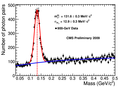
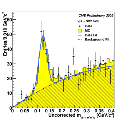
Figure 2: Left: Photon-pair invariant-mass distribution in the barrel ($|\eta|<$ 1.0) for the data. The $\pi^{0}$ mass peak is fitted with a Gaussian (red line) and the combinatorial background is described with an exponential function (blue line). Right: Invariant mass of $\pi^{0}$ candidates reconstructed as one photon and an e⁺ e^- pair. Data (black points) are superimposed on the MC expectation (filled yellow histogram), normalized to the number of selected conversion candidates. A fit to the data points, obtained with a Gaussian function summed with a second order polynomial to describe the combinatorial background component, is also shown.

4 Tracking

The CMS silicon tracker and tracking algorithms have performed excellently from the start of data taking. Beam spot and primary vertices are reconstructed with high efficiency and resolution close to the expectation from simulation $\!{}^{{\bf?}}$. Within hours after the first run with magnetic field switched on, invariant mass peaks were reconstructed of the decays of the neutral kaon $K_{S}^{0}\to\pi^{+}\pi^{-}$ and $\Lambda^{0}\to p\pi^{-}$ (and their charge conjugates), with a mass scale correct to better than 0.1%, and good agreement between data and simulation in resolution. The agreement in mass at low $p_{\rm T}$ is a new, independent, confirmation that the scale of the magnetic field is modeled accurately, and also provides a first indication that the description of material effects in the tracker is realistic.

As these particles are long-lived ($c\tau>1$ cm) and decay to a pair of charged particles, they provide a so-called $V^{0}$ signature, consisting of two oppositely charged tracks which are detached from the primary vertex and form a good vertex. To ensure good track quality, a track is required to have more than 5 hits, a normalized $\chi^{2}$ less than 5, and a transverse impact parameter with respect to the beamspot greater than $0.5\,\sigma_{\rm IP}$ where $\sigma_{\rm IP}$ is the calculated uncertainty (including beamspot and track uncertainties). The reconstructed $V^{0}$ decay vertex must have a $\chi^{2}$ less than 7 and a transverse separation from the beamspot greater than 15 $\sigma_{\rm T}$ where $\sigma_{\rm T}$ is the calculated uncertainty. If either of the daughter tracks have hits that are more than 4$\sigma_{3D}$ inside the $V^{0}$ vertex (toward the primary vertex), the $V^{0}$ candidate is discarded.

The mass resolution of the $V^{0}$ depends on $\eta$ as well as the decay vertex position and a single Gaussian was not a sufficiently accurate functional form for the signal. Therefore, a double Gaussian with the same mean was used to fit the signal. For the background shapes, a linear background was used for $\pi^{+}\pi^{-}$ and the function $a(m-m_{p}-m_{\pi})^{b}$ was used for the $p\pi^{-}$ spectrum. The $\pi^{+}\pi^{-}$ and $p\pi^{-}$ mass distributions, along with the overlaid fits, are shown in Fig. 3.

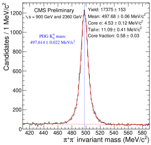
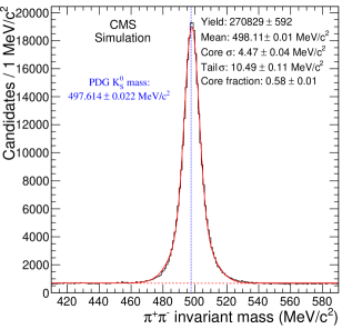
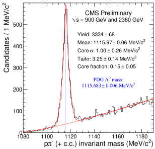
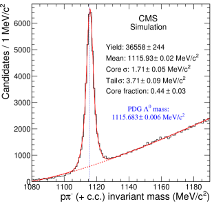
Figure 3: Fitted $\pi^{+}\pi^{-}$ mass for data (top left) and simulation (top right). Fitted $p\pi^{-}$ (+ charge conjugate) mass for data (bottom left) and simulation (bottom right). Uncertainties shown are statistical only.

Reconstruction of the $K^{*}(892)^{-}$, $\Xi^{-}$ and $\phi$ Resonances

The reconstructed sample of $V^{0}$ particles is exploited to search for other particles as well.

First, $K_{S}^{0}$ candidates are combined with charged tracks from the primary vertex to search for the strong decay $K^{*}(892)^{-}\to K_{S}^{0}\pi^{-}$. The $K_{S}^{0}$ candidates must have a mass within 20 MeV of the nominal PDG mass and the $K_{S}^{0}$ flight path must pass within 2 mm of the primary vertex. The $K_{S}^{0}\pi^{-}$ invariant mass is calculated using the PDG value of the $K_{S}^{0}$ mass and is shown in Fig. 4(left). The figure also shows an overlay of a fit to the $K_{S}^{0}\pi^{-}$ mass distribution. The fit uses a relativistic Breit-Wigner for the signal plus a threshold function for the background. More details are given elsewhere $\!{}^{{\bf?}}$. The mass returned by the fit is $888\pm 3$ MeV, consistent with the world average value of $891.66\pm 0.26$ MeV $\!{}^{{\bf?}}$.

The second particle, the $\Xi^{-}$, was reconstructed through its decay to $\Lambda^{0}\pi^{-}$. As the $\Xi^{-}$ is a long-lived baryon, the topology of this decay is different than the $K^{*}(892)^{-}$. The $\pi^{-}$ from the $\Xi^{-}$ decay will be detached from the primary vertex rather than originating from the primary vertex. $\Lambda^{0}$ candidates with a mass within 8 MeV of the PDG value were combined with charged tracks with the same sign as the pion in the $\Lambda^{0}$ decay (the track with the smallest $p_{\rm T}$). The resulting mass plot is shown in Fig. 4(right). The measured mass of $1322.8\pm 0.8$ MeV is in agreement with the world average value of $1321.71\pm 0.07$ MeV $\!{}^{{\bf?}}$.

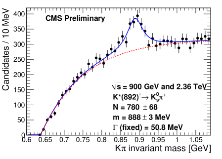
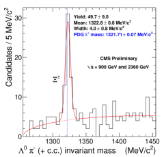
Figure 4: Left: $K_{S}^{0}\pi^{-}$ invariant mass plot with a fit for the $K^{*}(892)^{-}$. Right: $\Lambda^{0}\pi^{-}$ invariant mass plot with a fit for the $\Xi^{-}$.

Finally, a search for the $\phi$(1020)$\to K^{+}K^{-}$ resonance was performed, exploiting the possibility to separate kaons and pions at low $p_{\rm T}$ by measuring $dE/dx$ in the silicon detector layers. This analysis was described in a dedicated contribution to this conference $\!{}^{{\bf?},{\bf?}}$. Also in this case the mass that is fitted, $1019.58\pm 0.22$ MeV, is in good agreement with the PDG value of the $\phi$ mass of $1019.455\pm 0.020$ MeV. $\!{}^{{\bf?}}$ To conclude, all five resonances observed were found to have masses in agreement (to better than 0.1%) with the values listed in the PDG.

Table 1: Absolute and relative mass bias of several mass resonances observed in early CMS data, using track reconstruction and simulation out-of-the-box without any corrections. Only statistical uncertainties are included for the CMS results.

	$K^{0}_{S}$	$\Lambda^{0}$	$\Xi^{\pm}$	$K^{*\pm}$	$\phi$
Mass Bias (GeV)
$\Delta m=$
$(m_{\rm data}-m_{\rm PDG})-$	-0.37$\,\pm\,$0.07	0.04$\,\pm\,$0.06	0.0$\,\pm\,$0.9	-4.0$\,\pm\,$3.1	-0.22$\,\pm\,$0.26
$(m_{\rm MC}-m_{\rm gen})$
Relative bias (%)
$\Delta m/m_{\rm PDG}$	-0.074$\,\pm\,$0.014	0.004$\,\pm\,$0.005	0.00$\,\pm\,$0.07	-0.5$\,\pm\,$0.4	-0.02$\,\pm\,$0.03

Basic b-tagging Observables

A proper understanding of impact-parameter resolution of tracks and the reconstruction of secondary vertices is important for b-tagging, and presents the next challenge for the tracker and tracking algorithms. To validate the basic ingredients for b-tagging on a larger sample of events, a few changes to the reconstruction chain were applied $\!{}^{{\bf?}}$ with respect to the default algorithm $\!{}^{{\bf?}}$, relaxing the requirements on the acceptance of tracks, jets, and the matching between them. Figure 5(top left) shows the three-dimensional impact parameter significance distribution for all tracks in a selected sample of jets, computed with respect to the reconstructed primary vertex.

The secondary vertex reconstruction using the tracks associated to jets has also been slightly modified $\!{}^{{\bf?}}$, with relaxed requirements. To suppress $K_{S}^{0}$ candidates, the transverse secondary vertex separation was required to be less than 2.5 cm and the secondary vertex invariant mass more than 15 MeV from the nominal $K_{S}^{0}$ mass. The vertex flight distance is compared to what is expected from a simulation of minimum bias events in Fig. 5(top right). In general the agreement between data and simulation over the entire range of interest for the variables considered is remarkable. While many two- and three-track vertices are reconstructed, only one four-track vertex is expected (see Fig. 5, bottom left) and one is found in the data $\!{}^{{\bf?}}$. The corresponding event display is shown in the same figure (bottom right).

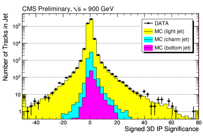
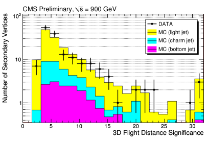
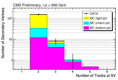
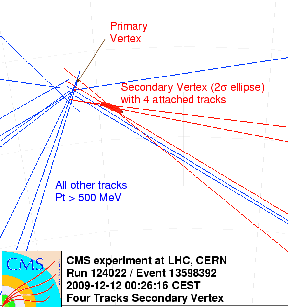
Figure 5: Distribution of the significance of the three-dimensional impact parameter for all tracks in the jet (top left) and the significance of the three-dimensional displacement of the secondary vertex (top right). The data is shown as black dots while for the simulation the contributions from light flavor, charm, and bottom are shown as filled histograms. The two outermost bins contain the respective histogram overflow. The number of tracks in a secondary vertex (bottom left), and the only event with a 4-track secondary vertex (bottom right).

5 Unification of Calorimetry and Tracking: the Particle Flow Approach

With its combination of a strong magnetic field, precise silicon tracker and an electromagnetic calorimeter with fine lateral segmentation the CMS design lends itself beautifully for the Particle Flow approach. In this approach one aims at reconstructing all stable particles in the event (i.e., electrons, muons, photons and charged and neutral hadrons) from the combined information from all CMS sub-detectors, to optimize the determination of particle types, directions and energies. Simulation studies have shown $\!{}^{{\bf?}}$ that in the case of CMS this can lead to an improvement of about a factor two in resolution for jets at low $p_{\rm T}$ ($<$50 GeV) and for missing transverse energy.

A key ingredient is the linking of tracks with corresponding energy clusters in the calorimeters. This was the first aspect to focus on once collision data became available. The angular matching between tracks and calorimeter deposits was shown to be reproduced very well by simulation $\!{}^{{\bf?}}$.

Once tracks and calorimeter clusters are matched in angle (or position), the measured track momentum can be compared to associated calorimeter energy for the combined electromagnetic (ECAL) and hadronic (HCAL) calorimeter clusters, as shown as a function of the track $p_{\rm T}$ in Fig. 6. Again data and MC simulation agree well. Since the ECAL energy scale was shown to be correct within 2% and the tracking momentum scale within 0.1%, one can derive from this plot that the HCAL response simulation is correct to better than 5%.

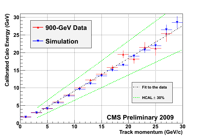
Figure 6: Average calorimeter response as a function of the track momentum for the 900 GeV data (red upwards triangles with error bars) and the corresponding minimum-bias simulation (blue downwards triangles with error bars), integrated over the full tracker acceptance ($|\eta|<2.4$). The dash-dotted line is a linear fit to the data, and the dashed lines show the same fit with a HCAL raw response changed by $\pm 30\%$, to guide the eye.

6 Jets and Missing Transverse Energy

In previous sections we have checked the calibration of all elements of tracking and calorimetry. These are used as ingredients for jet reconstruction. CMS uses the anti-$k_{\rm T}$ clustering algorithm $\!{}^{{\bf?}}$ with a cone size of 0.5 for commissioning, with three different types of inputs: Calo Jets are purely based on energy deposits in the calorimeter; Track Jets start from calo jets and use track information to improve the jet resolution; and Particle-Flow Jets use all particles reconstructed by the Particle Flow algorithm as input.

In all three cases, basic distribution of jet quantities were shown to be well reproduced by the simulation $\!{}^{{\bf?}}$. Using the same three types of input, CMS has started commissioning three algorithms for the determination of the missing transverse energy (MET), corresponding to the modulus of the vector sum of the transverse momenta of all reconstructed particles in the event $\!{}^{{\bf?},{\bf?}}$. The distributions of reconstructed MET for all three algorithms are shown in Fig. 7 (top row).

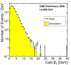
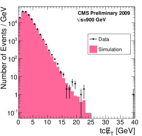
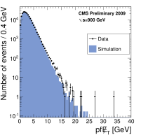
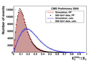
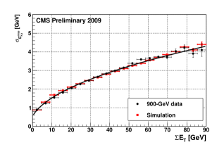
Figure 7: Top: reconstructed MET for caloMET (left), track-corrected MET (center) and particle-flow MET (right). Bottom: MET resolution estimated as MET/$\Sigma E_{\rm T}$ (left), and $E^{\rm miss}_{x,y}/\Sigma E_{\rm T}$ as a function of $\Sigma E_{\rm T}$ (right).

Since in this data sample no events are expected with invisible particles of significant transverse momentum, the distribution of MET/$\Sigma E_{\rm T}$ is a measure of the resolution of the MET determination, where $\Sigma E_{\rm T}$ is the scalar sum of the transverse energies of all particles in the event. This distribution, shown in Fig. 7(bottom left), gives a good indication of the improvement in resolution that can be achieved by using the Particle-Flow MET, compared to the calorimeter-only MET. Finally the resolution of the $x$- and $y$-component of MET, $E^{\rm miss}_{x,y}$ is plotted for Particle-Flow MET as a function of $\Sigma E_{\rm T}$, and can be parametrized as $\sigma(E^{\rm miss}_{x,y})=a\oplus b\sqrt{\Sigma E_{\rm T}}$, with $a$=0.55 GeV and $b$=45%, at $\sqrt{s}$= 900 GeV (Fig. 7, bottom right).

7 Transverse-momentum and pseudo-rapidity distributions of charged Hadrons

The good understanding of the tracker performance allowed a timely publication of the first physics measurement from collision data performed by CMS: the measurement of the inclusive charged-hadron transverse-momentum and pseudo-rapidity distributions in proton-proton collisions at $\sqrt{s}$ = 900 GeV and 2.36 TeV.$\!{}^{{\bf?}}$ For this measurement three different methods with different sensitivity to potential systematic effects were combined: pixel cluster counting, pixel tracklets, and full track reconstruction. As shown in Fig. 8(a), the tracking method allowed reconstruction of tracks down to very low transverse momentum. The other two methods allow the counting of charged hadrons to even lower values of $p_{\rm T}$. The combined pseudo-rapidity density result is shown in Fig. 8(b).

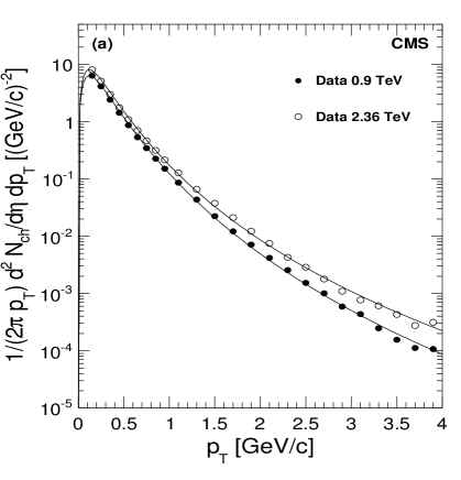
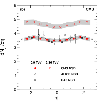
Figure 8: (a) Measured yield of charged hadrons for $|\eta|<2.4$ with systematic uncertainties (symbols), fit with an empirical function. (b) Reconstructed pseudo-rapidity density of charged particles averaged over the cluster counting, tracklet and tracking methods (circles), compared to data from the UA5 (open squares) and from the ALICE (open triangles) experiments at 0.9 TeV, and the averaged result over the three methods at 2.36 TeV (open circles). The CMS and UA5 data points are symmetrized in $\eta$. The shaded band represents systematic uncertainties of this measurement, which are largely correlated point-to-point. The error bars on the UA5 and ALICE data points are statistical only.

For non-single-diffractive interactions, the average charged-hadron transverse momentum was measured to be 0.46$\,\pm\,$0.01 (stat.)$\,\pm\,$0.01 (syst.) GeV at 0.9 TeV, and 0.50$\,\pm\,$0.01 (stat.)$\,\pm\,$0.01 (syst.) GeV at 2.36 TeV, for pseudorapidities $|\eta|<$2.4. At these energies, the measured pseudorapidity densities in the central region, dN ch/d$\eta$ for $|\eta|<$0.5, are 3.48$\,\pm\,$0.02 (stat.)$\,\pm\,$0.13 (syst.) and 4.47$\,\pm\,$0.04 (stat.)$\,\pm\,$0.16 (syst.), respectively. The results at 0.9 TeV are in agreement with previous measurements by UA5 $\!{}^{{\bf?}}$ and ALICE $\!{}^{{\bf?}}$, thus confirming the expectation of near equal hadron production in ${\rm p\bar{p}}$ and pp collisions. The results at 2.36 TeV represent the highest-energy measurements at a particle collider to date, at the time of this conference.

8 Conclusions

The CMS collaboration has extracted many useful performance results and one physics measurement from the first 10 $\mu$b^-1 of collision data delivered by the LHC. Several other physics analyses are in progress. The performance of the detector at start-up was outstanding. It should however be noted that the integrated luminosity recorded so far corresponds to less than a millisecond of data taking at the nominal LHC luminosity, which means that we are still many orders of magnitude away from a data sample with which CMS can begin to explore the physics for which the detector was designed.

Nevertheless, the first results indicate that CMS is in a very good shape to produce high quality physics results quickly once more data are recorded in the upcoming physics run at a collision energy of 7 TeV.

References

CMS Physics Analysis Summaries and Detector Performance Summaries are available at
http://cdsweb.cern.ch/collection/CMS

References

- [1] The CMS Collaboration, JINST 3, S08004 (2008).
- [2] Lyndon Evans and Philip Bryant (editors), JINST 3, S08001 (2008).
- [3] The CMS Collaboration, JHEP 02, 041 (2010)
- [4] The CMS Collaboration, JINST 5, T03001-T03022 and P03007 (2010).
- [5] The CMS Collaboration, CMS Detector Performance Summary, DPS-10-001 (2010).
- [6] The CMS Collaboration, CMS Physics Analysis Summary, PFT-10-001 (2010).
- [7] C. Amsler et al, Phys. Lett. B 667, 1 (2008).
- [8] The CMS Collaboration, CMS Physics Analysis Summary, EGM-10-001 (2010).
- [9] The CMS Collaboration, CMS Physics Analysis Summary, TRK-10-001 (2010).
- [10] Luca Perrozzi for the CMS Collaboration, these proceedings.
- [11] The CMS Collaboration, CMS Physics Analysis Summary, BTV-09-001 (2009).
- [12] The CMS Collaboration, CMS Detector Performance Summary, DPS-10-003 (2010).
- [13] The CMS Collaboration, CMS Physics Analysis Summary, PFT-09-001 (2009).
- [14] The CMS Collaboration, CMS Physics Analysis Summary, JME-10-001 (2010).
- [15] The CMS Collaboration, CMS Physics Analysis Summary, JME-10-002 (2010).
- [16] The UA5 Collaboration, Z. Phys. C 33, 1 (1986).
- [17] The ALICE Collaboration, Eur. Phys. J. C 65, 111 (2010).