Roles of Bond Alternation in Magnetic Phase Diagram of $R$MnO₃

Abstract

In order to investigate the nature of the antiferromagnetic structures in perovskite $R$MnO₃, we study a Heisenberg $J_{1}$-$J_{2}$ model with bond alternation using analytical and numerical approaches. The magnetic phase diagram which includes incommensurate spiral states and commensurate collinear states is reproduced. We discuss that the magnetic structure with spin $\uparrow\uparrow\downarrow\downarrow$ configuration (E-type structure) and the ferroelectricity emerge cooperatively to stabilize this phase. Magnetoelastic couplings are crucial to understand the magnetic and electric phase diagram of $R$MnO₃.

Strongly correlated electron systems show various phase transitions involving complex order parameters, in general. Typically, in perovskite manganites $R$MnO₃, phases with spin, charge, orbital and lattice degrees of freedom emerges and competes with each other, through control of carrier concentrations and ionic radius of $R$ ions.[1] In these Mn ions, 3d electrons exhibit varieties of phases in nearly identical systems with a slight change in a few set of parameters.

One of the recent topics in these $R$MnO₃ is the presence of multiferroic properties. For compounds with $R=$La, Nd, Sm, …, a spin A-type antiferromagnetic (A) phase is observed. In this phase, spins order ferromagnetically in the $ab$ plane and antiferromagnetically along $c$ axis, i.e., the magnetic ordering vector is ${\bm{q}}=(0,0,2\pi)$ in the orthorhombic lattice with GdFeO₃-type distortions. However, when one substitutes $R$ ions with smaller ones $R=$ Tb, Dy, …, an incommensurate spin spiral (ICS) phase emerges accompanied by ferroelectricity.[2, 3] In this phase, magnetic propagation vectors are along the $b$ axis, ${\bm{q}}=(0,q_{m},2\pi)$ where $0<q_{m}<\pi$. The origin of the ferroelectricity is the inverse Dzyaloshinsky-Moriya (DM) mechanism for the ICS structures.[4, 5, 6] Here, a local electric polarization is generated through the antisymmetric magnetoelectric (ME) coupling $\bm{P}_{ij}\propto\bm{e}_{ij}\times(\bm{S}_{i}\times\bm{S}_{j})$, where $\bm{S}_{i}$ is the spin direction at $i$-th site and $\bm{e}_{ij}$ denotes the unit vector connecting $i$ and $j$ sites. One of the experimental evidences is that the reorientations of $\bm{P}$ from $\bm{P}\parallel a$ to $\bm{P}\parallel c$ by chemical substitutions or application of magnetic fields are always accompanied by $ab$ to $bc$ cycloidal-plane flops.[7, 8]

Among various attempts to understand phase diagrams of $R$MnO₃,[3, 9] finite temperature phase diagrams including $ab$- and $bc$-cycloid phases have only been reproduced successfully by a model described as follows, so far: The model is a classical Heisenberg model defined on an three-dimensional orthorhombic lattice with nearest neighbor (n.n.) ferromagnetic exchanges $J_{1}$, and next nearest neighbor (n.n.n.) antiferromagnetic exchanges $J_{2}$, as well as single ion anisotropies and DM interactions.[10, 11] Models based on the $J_{1}$-$J_{2}$ Heisenberg model also explain spectra for magnons and electromagnons in these compounds.[12, 13, 14] Construction of a realistic and accessible microscopic model is quite appreciable from the viewpoint of comprehension of mechanisms as well as predictions and materials designs for novel phenomena.

For smaller ions at $R$=Ho, Tm, Lu, …, where $J_{2}/J_{1}$ is expected to be larger, spins exhibit an E-type antiferromagnetic (E) phase with spin $\uparrow\uparrow\downarrow\downarrow$ collinear structure along the $b$-axis with the magnetic propagation vector ${\bm{q}}=(0,\pi,2\pi)$. This phase also exhibits ferroelectricity $\bm{P}\parallel a$ and thus is multiferroic. It is considered that the ferroelectricity is driven by the E phase orderings through the symmetric ME coupling $|\bm{P}|\propto(\bm{S}_{i}\cdot\bm{S}_{j})$ of the magnetoelastic origin,[15, 16] as illustrated in Fig. 1.

The Heisenberg model with $J_{1}$-$J_{2}$ interactions alone, however, does not reproduce the E phase, as recently emphasized by Kaplan.[17] A possible way to stabilize the E phase is to introduce a uniaxial anisotropy which enhances collinear behaviors. The authors have studied the Heisenberg model with anisotropies and DM interactions, which successfully reproduces the A-ICS transition, in the large $J_{2}/J_{1}$ region.[11] Within the realistic range of parameters, however, we fail to observe the E phase. Another candidate is the biquadratic interaction which also enhances collinearity.[17] At this point, however, it is not clear weather such an interaction dominantly acts to stabilize the E phase in $R$MnO₃.

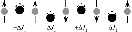
Figure 1: Schematic view of the lattice distortion in E-type spin structure phase of $R$MnO₃. Gray circle with arrow shows Mn ions with spin $\uparrow\uparrow\downarrow\downarrow$ structure. Displacement of oxygen ions (filled circle) gives rise to a uniform electric polarization. Due to the Goodenough-Kamamori mechanism, nearest neighbors exchanges are modulated as $\pm\Delta J_{1}$, which gives a gain in total energy for E-type phase.

In this paper, we introduce an alternative model to investigate the spin structures of $R$MnO₃. Namely, we study a classical Heisenberg model with bond alternations as a result of the magnetoelastic couplings mentioned above. We clarify that the model can reproduce the A-ICS-E phase transitions in $R$MnO₃, and discuss the nature of the ME phase diagram. Since $R$MnO₃ is a rare system which exhibits both symmetric and antisymmetric ME couplings E and ICS phases, respectively, it is also quite interesting to study the phase transition across these phases in order to make further comprehension for the ME effects in these compounds.

We study a classical Heisenberg model with spin exchange bonds depicted in Fig. 2 as

$${\cal H} =-\sum_{<i,j>}J_{ij}\bm{S}_{i}\cdot\bm{S}_{j}-J_{2}{\sum_{<i,j>}}^{\prime}\bm{S}_{i}\cdot\bm{S}_{j}$$

$$\qquad-J_{c}{\sum_{<i,j>}}^{\prime\prime}\bm{S}_{i}\cdot\bm{S}_{j}.$$ (1)

Here, the first summation is taken over n.n. bonds on the $ab$ plane, and $J_{ij}$ takes the alternating values along $b$-axis in the form

$$J_{ij}=J_{1}(1\pm\Delta),$$ (2)

as depicted in Fig. 2. Bond alternation parameter $\Delta$ is restricted within $0\leqq\Delta\leqq 1$. The second summation is for n.n.n. bonds along $b$-axis. We take $J_{1}>0$ (ferromagnetic) and $J_{2}<0$ (antiferromagnetic). The third term of the Hamiltonian is the inter-plane antiferromagnetic couplings along $c$-axis. At $T=0$, $J_{c}$ merely create staggered stacking of $ab$-plane spin structure along $c$-axis, and thus irrelevant for the phase diagrams with respect to $J_{1}$ and $J_{2}$. For example, it is determined automatically that a ferromagnetic alignment of spins in the $ab$ plane stack antiferromagnetically form the A-phase. Therefore, we may focus on spin structures within the $ab$ plane.

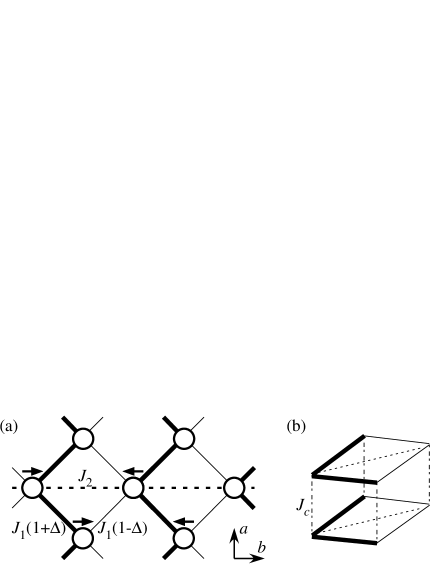
Figure 2: Bond alternating $J_{1}$-$J_{2}$ model, depicted on (a) the $ab$ plane and (b) the orthorhombic lattice. Thick and thin diagonal lines represent nearest neighbor bonds with exchange coupling $(1+\Delta)J_{1}$ and $(1-\Delta)J_{1}$, respectively. Dotted lines represent bonds with $J_{2}$. Interlayer antiferromagnetic coupling $J_{c}$ is shown by dash-dotted lines. $a$, $b$ and $c$ represent orthorhombic axes. Thick arrows in (a) depict a spin configuration in the E-type structure.

In the absence of the bond alternation $\Delta=0$, the model at $T=0$ gives an ordinary spiral state with $\theta_{n}=n\theta$, where $\theta_{n}$ describes the angle of the spin within the spiral plane. Here, $n$ describes the position of the spin along the propagation vector $\parallel b$. The rotation angle $\theta$ is determined by $\cos\theta=1/(2\gamma)$, where

$$\gamma=-J_{2}/J_{1},$$ (3)

and the $b$ component of the propagation vector is given by $q_{m}=2\theta$.

At $\Delta\neq 0$, staggered modulation of $J_{1}$ is introduced. Then we introduce a variational spin state with uniform and staggered component for the rotation angle

$$\theta_{n}=n\theta+(-1)^{n}\delta/2.$$ (4)

Total exchange energy per site scaled by $J_{1}$ is described by $\varepsilon(\theta,\delta)$, which is calculated as

$$\varepsilon(\theta,\delta) =-({1+\Delta})\cos(\theta-\delta)-({1-\Delta})\cos(\theta+\delta)$$

$$\qquad+\gamma\cos 2\theta-\gamma_{c},$$ (5)

where $\gamma_{c}=-J_{c}/J_{1}$. Minimization of $\varepsilon(\theta,\delta)$ with respect to $\delta$ and $\theta$ through $\partial\varepsilon/\partial\theta=\partial\varepsilon/\partial\delta=0$ leads to

$$\tan\delta =\Delta\tan\theta,$$ (6)

$$\cos\theta =\sqrt{\frac{1-\Delta^{2}}{4\gamma^{2}}-\frac{\Delta^{2}}{1-\Delta^{2}}}.$$ (7)

From Eq. (6) we have $\delta=0$ in the limit $\theta=0$ , which implies an A-phase, irrespective of $\Delta$. Similarly, at $\delta=\pi/2$ we have $\theta=\pi/2$ which makes a collinear E phase. Critical value of $\Delta$ for the A-ICS boundary is given from Eq. (7) at $\theta=0$ as

$$\Delta_{c}^{\rm(A)}=\sqrt{1-2\gamma},$$ (8)

whereas at $\theta=\pi/2$ we have the ICS-E boundary

$$\Delta_{c}^{\rm(E)}=\sqrt{\gamma^{2}+1}-\gamma.$$ (9)

Since $\Delta_{c}^{\rm(E)}>0$, E phase is stabilized only in the presence of the bond alternation $\Delta$. In Fig. 3 we show the phase diagram.

In order to justify the above analytical discussion, we perform the Monte-Carlo calculations at low temperatures. In the above, we have assumed the spin configuration of Eq. (4). On the other hand, the Monte-Carlo calculation does not restrict the spin configuration, and thus provides unbiased results. The calculation indeed confirms that only the three magnetic phases, i.e., A, ICS, and E phases are possible within our model so that the assumption of Eq. (4) is justified. As its consequence, the analytical results are precisely reproduced by the calculation.

In our numerical calculations, we also add the $\mathcal{H}_{D}=D\sum_{i}S_{zi}^{2}$, which makes magnetization along the $z$ axis hard. Because of this term, the spins in the ICS phase rotate in the $xy$ plane. This term makes the calculations stable by suppressing thermal fluctuations of the spiral plane without affecting the A-ICS-E transitions at $T=0$. We take $J_{c}/J_{1}$=1 and $D/J_{1}$=0.2 in the calculation. We analyze this model using the Monte-Carlo technique for systems with 48$\times$48$\times$6 sites with periodic boundaries.

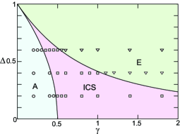
Figure 3: (Color online) Phase diagram of the alternate $J_{1}$-$J_{2}$ model at the ground state. A, E, and ICS denote A-type, E-type, and incommensurate spiral phases, respectively. Solid lines are the phase boundaries determined by the analytical calculation. Circle, triangle, and square symbols denote the points at which the A, E, and ICS spin structures are respectively obtained in the Monte-Carlo calculation at $T/J_{1}$=0.2.

The calculation successfully reproduces the analytically predicted phase diagram of Fig. 3. The circle, triangle and square symbols in Fig. 3 denote the points at which the A, E, and ICS spin structures are respectively obtained in the Monte-Carlo calculation at $T/J_{1}$=0.2.

These magnetic structures are assigned from the peak position of the spin correlation functions at ${\bm{q}}=(0,q_{m},2\pi)$. We also measure the spin-helicity correlation function to identity the phases. Here, the local spin-helicity vector is defined as $\bm{h}_{i}=(\bm{S}_{i}\times\bm{S}_{i+\hat{x}}+\bm{S}_{i}\times\bm{S}_{i+\hat{y}})/2S^{2}$ where $\hat{x}$ and $\hat{y}$ point the n.n. sites along [110] (pseudo-cubic $x$) and [-110] (pseudo-cubic $y$) directions, respectively. In spiral structures, the rotating spins give rise to a ferro-arrangement of the spin helicities, which results in a peak of the spin-helicity correlation at $\bm{q}$=0, while in collinear phases, the spin-helicity correlation has no peak structure.

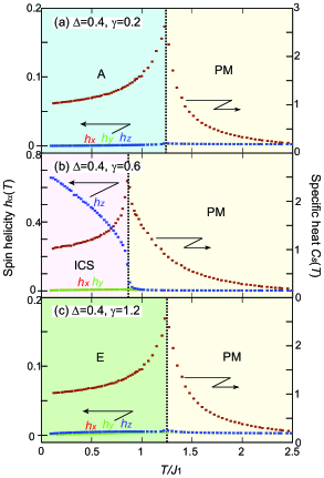
Figure 4: (Color online) Calculated temperature profiles of specific heat $C_{s}(T)$ and spin-helicity vector $\bm{h}_{s}(T)$ for typical points in the phase diagram where the ground states are estimated to be (a) A-type, (b) ICS, and (c) E-type. PM denotes the paramagnetic phase.

Let us now show some details of the calculation. In Fig. 4, we show the temperature dependence of specific heat $C_{s}(T)=(1/N)({\partial\langle\mathcal{H}\rangle})/({\partial(k_{\rm B}T)})$, as well as the spin-helicity vector $\bm{h}_{s}(T)$ where $h_{\alpha}(T)$ ($\alpha$=$x$, $y$ and $z$) denotes the $\alpha$ component of the spin-helicity vector, at (a) ($\Delta$, $\gamma$)=(0.4, 0.2), (b) ($\Delta$, $\gamma$)=(0.4, 0.6), and (c) ($\Delta$, $\gamma$)=(0.4, 1.2) where the ground states are predicted to be (a) A-type, (b) ICS, and (c) E-type, respectively —– see also the phase diagram in Fig. 3.

In all cases, we can see a single phase transition from paramagnetic (PM) phase at high temperatures to each ordered phase at low temperatures, at which $C_{s}(T)$ exhibits a sharp peak. We also confirm that the choice of $T/J_{1}=0.2$ gives a sufficiently low-temperature state.

In the present calculation, the spins in the ICS phase rotate in the $xy$ plane since we incorporate the hard-axis type spin anisotropy along the $z$ axis in the Hamiltonian. Under this circumstance, $h_{z}(T)$ has a large value, while $h_{x}(T)$ and $h_{y}(T)$ are almost zero. We can indeed see that $h_{z}(T)$ starts increasing at the transition to the ICS phase in Fig. 4(b). On the other hand, as shown in Figs. 4(a) and  4(c), $z$ component of the helicity is as small as other components in the collinear spin phases.

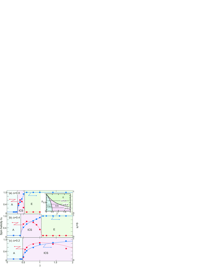
Figure 5: (Color online) Calculated $\gamma$ dependence of the momentum $q_{m}/\pi$ at which the spin correlation function has a peak at $T/J_{1}$=0.2, and $\gamma$ dependence of the spin-helicity $z$ component $h_{z}$ at $T$=0 for (a) $\Delta$=0.6, (b) $\Delta$=0.4, and (c) $\Delta$=0.2. The data of $h_{z}$ at $T$=0 are obtained by extrapolating the calculated temperature profile of $h_{z}(T)$. Solid and dashed lines are $q_{m}/\pi$ and $h_{z}$ obtained from the analytical approach.

In Fig. 5, we show the calculated $\gamma$ dependence of the momentum $q_{m}/\pi$ as well as the spin-helicity $h_{z}$ for (a) $\Delta$=0.6, (b) $\Delta$=0.4, and (c) $\Delta$=0.2. The data for the spin-helicity are obtained by extrapolating the calculated temperature profile of $h_{z}(T)$ to $T/J_{1}\to 0$. Those data as functions of $\gamma$ consistently exhibit A-ICS-E phase transitions, at least qualitatively.

Furthermore, let us compare these data with the variational spin structure given in Eq. (4). The spin structure gives $q_{m}=2\theta$ and $h_{z}=\sin\theta\cos\delta$, where $\theta$ and $\delta$ are determined by Eqs. (6) and (7). As plotted in Fig. 5, the Monte-Carlo data for $q_{m}$ and $h_{z}$ agree well with the analytical results given by solid and dashed lines, respectively.

So far we have confirmed that the spin structure given in Eq. (4) as well as the A-ICS-E phase transition derived from that is quite valid. Then we proceed to consider the case that the bond alternation is driven by lattice distortions to minimize the total energy. We assume that a lattice distortion $r$ creates the bond alternation $\Delta=gr$ with $g$ being the coupling constant. Total energy is given by a sum of the spin exchange energy $\varepsilon_{\rm s}(\Delta,\gamma)$ and an elastic energy $\propto r^{2}$, or equivalently

$$\varepsilon_{\rm tot}=\varepsilon_{\rm s}(\Delta,\gamma)+\frac{\Delta^{2}}{2\lambda^{2}}.$$ (10)

Here, $\lambda$ is the dimensionless spin-lattice coupling constant. Hereafter, we refer to the model as Peierls $J_{1}$-$J_{2}$ model.

The spin exchange energy is derived by applying Eqs. (6) and (7) to Eq. (5). In the A phase at $\Delta<\Delta_{c}^{\rm(A)}$, the minimized energy is derived from $\theta=\delta=0$ as

$$\varepsilon_{\rm s}(\Delta,\gamma)=-2+{\gamma}-\gamma_{c},$$ (11)

while in the E phase at $\Delta>\Delta_{c}^{\rm(E)}$, we have $\theta=\delta=\pi/2$ so that

$$\varepsilon_{\rm s}(\Delta,\gamma)=-2\Delta-{\gamma}-\gamma_{c}.$$ (12)

In the ICS phase at $\Delta_{c}^{\rm(A)}<\Delta<\Delta_{c}^{\rm(E)}$, we have

$$\varepsilon_{\rm s}(\Delta,\gamma)=-\frac{1-\Delta^{2}}{2\gamma}+\gamma\frac{1+\Delta^{2}}{1-\Delta^{2}}-\gamma_{c}.$$ (13)

Bond alternation $\Delta$ is determined by minimizing $\varepsilon_{\rm tot}$ with respect to $\Delta$ within the range $0\leqq\Delta\leqq 1$. The result in the region $\gamma>1/2$ can be summarized as follows. In Fig. 6, we schematically depict $\varepsilon_{\rm tot}$ as a function of $\Delta$ for various $\lambda$. We observe a transition from ICS phase to E phase at a critical coupling $\lambda_{\rm c}$ given by

$$\lambda_{\rm c}{}^{2}=1/({2\gamma}).$$ (14)

Here, $\varepsilon_{\rm tot}$ have degenerate energy minimums at $\Delta=0$ (ICS region) and at $\Delta>\Delta_{c}^{\rm(E)}$ (E region). As $\lambda$ is changed across $\lambda_{\rm c}$, we have a jump in the value of $\Delta$ for the energy minimum and thus the transition is first ordered. Furthermore, there exists a characteristic coupling

$$\lambda_{1}{}^{2}=\sqrt{\gamma^{2}+1}-\gamma,$$ (15)

where E phase has a local minimum in its energy with respect to $\Delta$ at $\lambda>\lambda_{1}$. This implies an existence of a metastable E state at $\lambda>\lambda_{1}$. Similarly, we also have

$$\lambda_{2}{}^{2}=2{\gamma}/({4\gamma^{2}-1}),$$ (16)

where an ICS state at $\Delta=0$ is metastable at $\lambda<\lambda_{2}$. Therefore, in the case $\gamma>1/2$, we may have coexistence of the ICS and the E phases at $\lambda_{1}<\lambda<\lambda_{2}$.

Similarly, in the case $\gamma\leqq 1/2$, 2nd order transition between the A and the ICS phases is observed at $\lambda_{c}$, while the metastable E state exist at $\lambda>\lambda_{1}$. The A states is always metastable at $\lambda>\lambda_{c}$ in this case. The forms for $\lambda_{c}$ and $\lambda_{1}$ coincide with those for the previous case given in Eqs. (14) and (15), respectively. The phase diagram is summarized in Fig. 6.

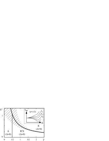
Figure 6: Phase diagram of the Peierls $J_{1}$-$J_{2}$ model. The solid curve shows the first-order phase boundary between E phase and ICS (F) phase at $\gamma>1/2$ ($\gamma<1/2$). The vertical solid line at $\gamma=1/2$ shows the second-order phase boundary between ICS and F phases. Hatched area shows the coexistence region. Inset: Total energy $\varepsilon_{\rm tot}$ as a function of $\Delta$ plotted in arbitrary units, for the case of $\gamma>1/2$. Dimensionless coupling constant $\lambda$ is increased from top to bottom, as $\lambda<\lambda_{1}$, $\lambda=\lambda_{1}$, $\lambda=\lambda_{c}$, $\lambda=\lambda_{2}$ and $\lambda>\lambda_{2}$, respectively.

Let us now compare these results with the magneto-electric properties in $R$MnO₃. In these compounds, commensurate E phase is always accompanied with ferroelectricity, which is consistent with our result that E phase is stabilized only at $\Delta\neq 0$. Although it has previously been discussed that ferroelectricity is triggered by magnetic E phase through lattice distortions, our result suggests that the magnetic E phase and ferroelectricity cooperatively emerge to stabilize themselves. Therefore, Peierls-type spin-lattice couplings are essentially important to understand the electric as well as the magnetic phase diagram of $R$MnO₃. Recent report shows that, in $R$MnO₃ there exists a region of possible coexistence for ICS and E phases.[18] The Peierls model discussed here indeed shows such a coexistence at around the 1st-order transition points between ICS and E phases. Experimental data in further details should give crucial tests for our present results. Theoretical approaches based on more realistic models including anisotropies, DM and biquadratic interactions should also be important to understand the whole phase diagrams of $R$MnO₃ in detail.

The author would like to thank S. Miyahara for stimulating discussions, as well as S. Ishiwata, Y. Taguchi and Y. Tokura for suggestions from experimental points of view. This work was partially supported by Grant-in-Aid for Scientific Research as well as High Tech Research Center Project from the MEXT, Japan.

References

- [1] For a review, “Colossal Magnetoresistive Oxides”, ed. by Y. Tokura (Gordon & Breach Science Publisher, 2000).
- [2] T. Kimura, T. Goto, H. Shintani, K. Ishizaka, T. Arima and Y. Tokura: Nature 426 (2003) 55.
- [3] T. Kimura, S. Ishihara, H. Shintani, T. Arima, K. T. Takahashi, K. Ishizaka, and Y. Tokura: Phys. Rev. B 68 (2003) 060403.
- [4] H. Katsura, N. Nagaosa, and A. V. Balatsky: Phys. Rev. Lett. 95 (2005) 057205.
- [5] I. A. Sergienko and E. Dagotto: Phys. Rev. B 73 (2006) 094434.
- [6] M. Mostovoy: Phys. Rev. Lett. 96 (2006) 067601.
- [7] Y. Yamasaki, H. Sagayama, T. Goto, M. Matsuura, K. Hirota, T. Arima, and Y. Tokura: Phys. Rev. Lett. 98 (2007) 147204.
- [8] Y. Yamasaki, H. Sagayama, N. Abe, T. Arima, K. Sasai, M. Matsuura, K. Hirota, D. Okuyama, Y. Noda, and Y. Tokura: Phys. Rev. Lett. 101 (2008) 097204.
- [9] S. Dong, R. Yu, S. Yunoki, J.-M. Liu, and E. Dagotto: Phys. Rev. B 78 (2008) 155121.
- [10] M. Mochizuki and N. Furukawa: J. Phys. Soc. Jpn. 78 (2009) 053704.
- [11] M. Mochizuki and N. Furukawa: Phys. Rev. B 80 (2009) 134416.
- [12] S. Miyahara and N. Furukawa: preprint, arXiv:0811.4082.
- [13] R. Valdés Aguilar, M. Mostovoy, A. B. Sushkov, C. L. Zhang, Y. J. Choi, S-W. Cheong, and H. D. Drew: Phys. Rev. Lett. 102 (2009) 047203.
- [14] M. Mochizuki, N. Furukawa and N. Nagaosa: arXiv:1001.3905.
- [15] T. Arima, A. Tokunaga, T. Goto, H. Kimura, Y. Noda, and Y. Tokura: Phys. Rev. Lett. 96 (2006) 097202.
- [16] Ivan A. Sergienko, Cengiz Sen and Elbio Dagotto: Phys. Rev. Lett. 97 (2006) 227204.
- [17] T.A. Kaplan: Phys. Rev. B80 (2009) 012407.
- [18] S. Ishiwata, Y. Kaneko, Y. Tokunaga, Y. Taguchi, T. Arima and Y. Tokura: arXiv:0911.4190.