The stellar content of the Hamburg/ESO survey

We determine the metallicity distribution function (MDF) of the Galactic halo based on metal-poor main-sequence turnoff-stars (MSTO) which were selected from the Hamburg/ESO objective-prism survey (HES) database. Corresponding follow-up moderate-resolution observations (R $\backsim$ 2000) of some 682 stars (among which 617 were accepted program stars) were carried out with the 2.3m telescope at the Siding Spring Observatory (SSO). Corrections for the survey volume covered by the sample stars were quantitatively estimated and applied to the observed MDF. The corrections are quite small, when compared with those for a previously studied sample of metal-poor giants. The corrected observational MDF of the turnoff sample was then compared with that of the giants, as well as with a number of theoretical predictions of Galactic chemical evolution, including the mass-loss modified Simple Model. Although the survey-volume corrected MDFs of the metal-poor turnoff and the halo giants notably differ in the region of $\mbox{[Fe/H]}>{-2.0}$, below $\mbox{[Fe/H]}\sim{-2.0}$, (the region we scientifically focus on most) both MDFs show a sharp drop at $\mbox{[Fe/H]}\sim{-3.6}$ and present rather similar distributions in the low-metallicity tail. Theoretical models can fit some parts of the observed MDF, but none is found to simultaneously reproduce the peak as well as the features in the metal-poor region with $\mathrm{[Fe/H]}$ between $-2.0$ to $-3.6$. Among the tested models only the GAMETE model, when normalized to the tail of the observed MDF below $\mbox{[Fe/H]}\sim{-3.0}$, and with $Z_{cr}=10^{-3.4}Z_{\odot}$, is able to predict the sharp drop at $\mbox{[Fe/H]}\sim{-3.6}$.

1 Introduction

The Galactic halo provides important clues for understanding the evolution and structure of the Galaxy. In the past few decades, considerable observational and theoretical efforts have been made to investigate its chemical evolution, details of its structure, and its kinematical characteristics. Very metal-poor stars in the halo, those with metallicity $\mathrm{[Fe/H]}$ $\lesssim-2.0$, are regarded as fossils of the earliest generations of stars. They preserve the chemical information created by their stellar progenitors, providing fundamental insights regarding the properties of the very first generation of stars, the chemical history of our Galaxy (and other large spirals like it), the modes of star formation in the proto-Milky Way, the formation of the Galactic halo, and physical mechanisms such as feedback processes in the early stages of galaxy evolution. Although we are gaining a deeper understanding over time, much remains to be explored. It is particularly revealing that, after many decades of assuming that the Galactic halo comprises a single stellar population, recent work (Carollo et al. 2007, 2010) has provided additional support to suspicions that emerged from previous efforts that the halo is indeed divisible into two structural components, with notably different spatial density profiles, stellar orbits, and stellar metallicities.

Recently, new theoretical models (e.g., Helmi 2008; Prantzos 2008; Salvadori et al. 2010) and observational constraints (e.g., Carollo et al. 2007, 2010; Bell et al. 2008; Ivezić et al. 2008; Jurić et al. 2008; Bond et al. 2009; de Jong et al. 2010) have greatly enhanced our understanding of the nature of the halo components of our Galaxy, Those are enabling the development of plausible assembly histories based on the degree of detectable spatial and phase-space substructures. The possible association of at least some presently observed dwarf galaxies with the formation of the halo populations, as invoked by Carollo et al. (2007) to account for their dual halo structure, has received additional support based on high-resolution spectroscopic analysis of individual stars in ultra-faint and dwarf spheroidal galaxies(e.g., Muñoz et al. 2006; Kirby et al. 2008; Geha et al. 2009; Frebel et al. 2010; Norris et al. 2010). Finally, the identification and detailed analysis of the elemental abundance patterns for the most chemically primitive stars, e.g., the ultra ($\mbox{[Fe/H]}<{-4.0}$; Norris et al. 2007) and hyper ($\mbox{[Fe/H]}<{-5.0}$; Christlieb et al. 2002; Frebel et al. 2005; Aoki et al. 2006) metal-poor stars allow one to trace back close to the very beginning of star formation in the Galaxy.

The observed metallicity distribution function (MDF) of halo stars provides strong constraints on models for the formation and chemical evolution of the Galaxy. Any accepted model must be able to predict the relative numbers of halo stars as a function of their metallicity (Beers & Christlieb 2005; Helmi 2008), and in the case of a dual-halo model, as a function of location and kinematics. Early investigations on the shape of the halo MDF were hampered by the small numbers of very metal-poor stars known at the time (Hartwick 1976; Bond 1981; Ryan & Norris 1991; Carney et al. 1996). Other attempts (e.g., Bonifacio et al. 2000; Schuster et al. 2004), based on samples of metal-poor stars from the HK survey of Beers and colleagues (Beers et al. 1985, 1992), suffer from poorly constrained selection criteria, except perhaps at the lowest metallicities. More recent efforts have made use of statistically well-understood selection criteria to identify large numbers of metal-poor candidates from objective-prism surveys, such as the Hamburg/ESO survey (HES – Wisotzki et al. 1996), as reported in a series of papers (Barklem et al. 2005; Christlieb et al. 2008; Schörck et al. 2009; Placco et al. 2010). Schörck et al. (2009), for example, used a sample of 1638 metal-poor giants to study the shape of the low-metallicity tail of the halo MDF, and made detailed comparisons with MDFs of Galactic globular clusters and satellite galaxies, as well as with theoretical models.

Main-sequence turnoff (MSTO) stars have long been used to explore Galactic structure, including the recognition of stellar substructures in the Galactic halo (Majewski et al. 2004; An et al. 2009), searches for kinematic streams (e.g., Klement et al. 2009), and statistical analyses of the amount of cold halo substructure in the Milky Way (e.g., Schlaufman et al. 2009). In addition, MSTO stars have also been proven important to the field of Galactic chemical evolution, through the analysis of high-resolution, high signal-to-noise spectroscopic observations to derive elemental abundances for metal-poor dwarf stars (Cohen et al. 2004), chemically interesting metal-poor turnoff stars (Aoki et al. 2008), and investigations of the so-called Spite Plateau (Spite & Spite 1982) through Li abundance measurements for metal-poor turnoff stars(Aoki et al. 2009; Sbordone et al. 2010). In this paper we construct the MDF of Galactic halo MSTO stars based on follow-up moderate-resolution ($R\sim 2000$) spectroscopic observations of candidate metal-poor turnoff stars from the HES. We also compare our results with the previously derived MDF of HES giants, and with theoretical expectations.

This work is a continuation of the HES stellar content series (Paper I – Christlieb et al. 2001b, II – Christlieb et al. 2001a, III – Christlieb et al. 2005, IV – Christlieb et al. 2008, V – Schörck et al. 2009). We describe the selection of the HES turnoff sample in Section 2, with details of the metallicity determination and MDF construction given in Section 3. The observed HES MSTO MDF is compared with theoretical predictions in Section 4; the main results are summarized in Section 5.

2 The Sample

Adopting the methods described in Paper IV, the HES metal-poor turnoff candidates were selected from the HES objective-prism database, using both KP/$(B-V)_{0}$ and KP/$(J-K)_{0}$ selections. The only exception was that an additional $(B-V)_{0}$ range was specified so that the candidates were restricted to 0.3 $\leq$ $(B-V)_{0}$$\leq$ 0.5. The KP index hereby measures the strength of the Ca ii K line and is defined in detail in Beers et al. (1999)). It was measured in all HES prism spectra and together with a color, the prime indicator for the selection of metal-poor candidates.

As shown in Figure 6 of Paper IV, the employed KP cutoff becomes comparable to its measurement uncertainty for stars within our $(B-V)_{0}$ range. Since turnoff stars are also relatively weak-lined, we thus included only those candidates whose Ca ii K line is not significantly detected in HES spectra, even if their KP indices are above the formal cutoff line. To maintain relatively consistent exposure times during the follow-up observations, an additional cutoff regarding the brightness of $B_{HES}\leq 16.5$ was adopted. The above cuts yielded a preliminary sample of 3383 metal-poor turnoff candidates from the HES database.

In order to provide candidates with a higher likelihood of being metal-poor, the HES prism spectra of the selected 3383 candidate were visually inspected. As defined in Paper IV, based on the apparent strength of the Ca ii K line relative to the continuum, the 3383 candidates were classified into four different metal-poor classes, mpca, unid, mpcb, and mpcc. The distributions of the 3383 candidates for these classes are listed in the second column of Table 1.

For accurate measurements of stellar metallicities (as well as the estimates of other stellar atmospheric parameters), moderate-resolution follow-up spectra are required. To avoid possible systematic offsets of spectral features that could arise from combining different telescope/detector combinations, we exclusively adopted data observed during 15 individual runs at the Siding Spring Observatory (SSO) 2.3m telescope with the Double Beam Spectrograph (DBS). The runs took place between January 2006 and November 2009. The resolving power was R $\backsim$ 2000, with a typical S/N of 20/1 per pixel in the continuum region close to the Ca ii K line.

For a total of 682 unique stars from our metal-poor turnoff candidate list follow-up spectra were obtained. The third column of Table 1 lists the numbers of these observed candidates for all four metal-poor classes. It is clear that a significant bias against the class mpcc exist because it is the subjectively least promising candidate class for finding metal-poor stars.

Table 1: Numbers of different metal-poor classes among the candidate HES turnoff sample, the sample with follow-up observations from SSO, and the accepted sample after the visual inspection and rejection as described in Section 3.1. The column labelled ”Factor” refers to the scaling factor used to construct the MDF described in Section 3.1

Class	HES prism	SSO follow-up	Accepted	Factor
mpca	179	36	29	6.17
unid	333	67	59	5.64
mpcb	1666	560	513	3.25
mpcc	1205	19	16	75.31
Total	3383	682	617

3 Analysis of the Observational Sample

3.1 Measurements of line indices and [Fe/H]

Line indices (Beers et al. 1999) were measured for all 682 stars in our program sample which include the KP index, the HP2 index (which measures the strength of the Balmer $H_{\delta}$ line), and the GP index (which measures the strength of the of CH G-band feature). In the cases where we had multiple spectra for a single object, we adopted a S/N-weighted average of the individual indices. Following this step, a visual inspection of the follow-up spectra was carried out to identify and reject spectra of objects that were too noisy, had emission lines present, or were too hot (as indicated by their Balmer line index); a few additional objects that turned out to be galaxies or were otherwise peculiar were rejected as well. No stars with GP $>$ 6 Å, which indicates strong spectral carbon features, were detected in our sample. This is perhaps not surprising, given the relatively high effective temperatures of our turnoff sample. We note that HE 1327$-$2326, the most metal-deficient star currently known, was one of the candidates observed during the 15 runs. On the grounds that the star was known to be hyper-metal-poor and in order to obtain a better medium-resolution spectrum than previously existed, it was included in the follow-up observations described here. However, we removed it from our sample because including this star might introduce a bias to the sample. This left us with an “accepted” sample containing 617 stars, with the distribution across different metal-poor classes given in Column 4 of Table 1.

To obtain $\mathrm{[Fe/H]}$ estimates for the stars in our sample, two independent procedures were carried out. The first obtains $\mathrm{[Fe/H]}$ from the measured KP and HP2 indices by using an updated code version making use of the methods described by Beers et al. (1999) (which includes more calibration stars, and thus results in a better coverage of stellar parameter space, especially in the lowest metallicity regime). This was the method used in Paper V when constructing the giant-star sample. The second method is a newly developed version of the SEGUE Stellar Parameter Pipeline (SSPP - Lee et al. 2008a, b; Allende Prieto et al. 2008). The SSPP is the software tool used to obtain estimates of atmospheric parameters for stellar spectra obtained during the course of the Sloan Digital Sky Survey (York et al. 2000; Abazajian et al. 2009) and its extensions, SDSS-II and SDSS-III. Recent experiments with spectral data with similar resolving power to SDSS spectra ($R=2000$) have indicated that the SSPP can provide useful estimates of parameters for non-SDSS data as well, as long as the wavelength coverage extends from roughly 3800 Å to 5200 Å. Slightly smaller wavelength ranges can still be used, but the accuracy of the derived parameters (in particular surface gravity) begins to suffer when the red limit is less than 5000 Å, due to the loss of the Mg I$\mathrm{b}$ and MgH features, which provide enhanced sensitivity to estimates of $\log$ g.

The non-SEGUE Stellar Parameter Pipeline (n-SSPP) takes as inputs user-supplied measurements or estimates of the Johnson $V$ magnitude and $B-V$ color, and/or a 2MASS (Cutri et al. 2003) $J$ magnitude and $J-K$ color, all corrected for a user-specified level of absorption and reddening, along with a user-supplied estimate of the observed radial velocity. It then proceeds to determine estimates of the primary atmospheric parameters ($T_{\mbox{\scriptsize eff}}$, $\log$ g, $\mathrm{[Fe/H]}$) and their estimated errors, as well as estimates of distance, making use of a subset of the procedures described in Lee et al. (2008a) (i.e., those that can be made to work within the wavelength region covered by the input spectrum). Note that it is not necessary that the input spectra be flux calibrated, nor continuum rectified. It is also not strictly necessary to supply input colors, since the n-SSPP makes internal estimates that can be used as needed, but due to possible degeneracies in the derived parameters color information is certainly preferred.

The n-SSPP was used to obtain atmospheric parameter estimates for our 617 accepted program stars. Input Johnson colors were taken from the estimates provided by the HES catalog (for $V$ and $B-V$), or photometric measurements for a small subset of the data available from Beers et al. (2007) or later (Beers et al., in prep.); $J$ and $J-K$ were taken from the 2MASS Point Source Catalog, absorption corrected or de-reddened according to the Schlegel et al. (1998) dust maps.

Figure 1: Comparison of the metallicities ($\mathrm{[Fe/H]}$) of the HES turnoff sample measured with the updated version of the Beers et al. (1999) method and the n-SSPP. The dashed line is the one-to-one line; typical errors for both measurements are shown in the upper-left corner. A slight offset between the methods is clearly present. See text for discussion.

The resulting estimates of $\mathrm{[Fe/H]}$ for the two methods are compared in Figure 1. Although the two measurements do not greatly differ, the typical error of the Beers et al. (1999) determination (0.18 dex) is twice that of the n-SSPP estimate (0.09 dex). The determination based on Beers et al. (1999) exhibits an offset in $\mathrm{[Fe/H]}$ compared with the n-SSPP of $-0.19\pm 0.01$, resulting in a metallicity distribution that reaches apparently lower $\mathrm{[Fe/H]}$. In order to make the derived metallicity distribution as accurate as possible we have adopted the high-resolution measurements for the three candidates that have been observed with high-resolution spectroscopy (Cohen et al. 2004). As shown in Table 2, the metallicities obtained by the n-SSPP for these stars are closer to the values derived by the high-resolution analysis than are those from the Beers et al. approach. Considering the fact that the n-SSPP procedure delivers what is likely to be a more accurate estimate of $\mathrm{[Fe/H]}$, the following statistical discussion will be based on this method.

Table 2: Comparisons of difference measurement techniques for $\mathrm{[Fe/H]}$. Columns 2-4 respectively refer to values derived by the updated version of the Beers et al. (1999) method, the n-SSPP, and detailed analysis by Cohen et al. (2004) based on high-resolution spectroscopy.

HES ID	$\mbox{[Fe/H]}_{1}$	$\mbox{[Fe/H]}_{2}$	$\mbox{[Fe/H]}_{3}$
HE 0007-1832	$-$3.32	$-$2.98	$-$2.65
HE 0105-2202	$-$2.87	$-$2.86	$-$2.55
HE 1346-0427	$-$3.32	$-$3.57	$-$3.40

Distances to our sample stars were calculated by assigning the stars into various luminosity classes. This was done based on the surface gravity estimates derived by the n-SSPP. We considered all stars with estimated log g $\geq 3.5$ to be likely dwarfs, those with 3.5 $<$ log g $\leq$ 3.0 to be turnoff stars, and those with log g $<$ 3.0 to be subgiants and giants. The distribution of the sample in the Z-R plane is shown in Figure 2. It indicates that our sample of turnoff candidates is indeed located within $2-3$ kpc of the Sun. This can be contrasted with a similar figure (Figure 3) from Paper V which shows that the giants are located at much larger distances from the Sun.

Figure 2: Spatial distribution of the observed HES MSTO sample. R indicates the Galactocentric distance projected to the plane; Z indicates the distance above or below the Galactic plane. In this diagram, the Sun is assumed to be located at R = 8 kpc, Z = 0.

3.2 Observational biases and selection effects

Before comparing our observed MDF with other results or theoretical predictions, it is necessary to address the biases and selection effects that are introduced through the survey itself or by our sample selection procedure.

One notable selection bias comes from the metal-poor classification. As shown in Figure 3 the follow-up observations clearly favor the best metal-poor candidates. The numbers in the panels indicate that the relative selection efficiency of extremely metal-poor (EMP) stars ($\mbox{[Fe/H]}\leq{-3.0}$) obviously decreases from a maximum of about 10% for the better candidate classes, mpca and unid, to the least likely class, mpcc. Note that the fraction of EMP stars in class mpca is somewhat lower than that in class unid, probably due to the fact that turnoff metal-poor stars are rather weak-lined, making the divisions between these classes rather difficult. The numbers of targets in mpcc is rather small (16), hence it is perhaps not surprising that no EMP stars were found in this class.

Figure 3: The observed MDFs of the different metal-poor classes. The numbers listed in each panel correspond to the number of EMP stars (the numerator) compared to the total number of stars in the corresponding class (the denominator).

3.3 Construction of the MDF

As discussed above, the MDF derived from our follow-up observations contains a significant bias towards the more metal-deficient candidates, and must be taken into account to recover a reasonable representation of the “true” MDF. Therefore, we adopted the scaling factor procedure described in Paper V. For each metal-poor class, the MDF of the observed candidates is scaled by a factor calculated from the division of the total number in the class by the observed number (as listed in the last column in Table 1). Then the scaled MDFs of the four classes are co-added to produce a general MDF for the entire HES candidate sample. Similarly to Paper V, the main difference between the directly observed and the scaled MDF is the increasing ratio of the relatively metal-rich stars in the mpcb and mpcc classes. The normalized fraction of the scaled MDF is listed in the first column of Table 3.

3.4 Selection fraction

As pointed out in Paper IV and V, the combination of the KP index with $(B-V)_{0}$  or $(J-K)_{0}$  for the purpose to select metal-poor candidates in the HES has proven rather efficient. Following the metallicity distribution predicted by the Simple Model, we apply our quantitative selection criteria to a simulated sample of metal-poor stars. The results of the theoretical selection fractions shown in Figure 4. The selection fractions for both $(B-V)_{0}$ and $(J-K)_{0}$  are shown. It is clear that the selection criteria are able to reject the majority of stars with $\mathrm{[Fe/H]}$ greater than $-2.0$. For both colors, a high completeness (up to almost 100%) is reached for stars with $\mbox{[Fe/H]}\leq{-3.0}$. For $(B-V)_{0}$, the redder candidates exhibit a larger selection fraction (due to less contamination from hot stars among the bluer candidates). The selection fraction, however, does not differ much among the different $(J-K)_{0}$  cutoffs. This is as expected since the blue cutoff in $(J-K)_{0}$ is already fairly red so that fewer hot candidates enter the sample.

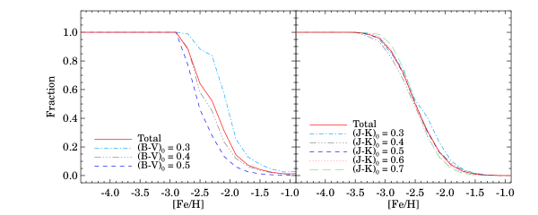
Figure 4: Selection fractions of metal-poor candidates selected with the HES selection criteria as described in Paper IV. The two panels correspond to selection efficiencies using KP and $(B-V)_{0}$ (left) or $(J-K)_{0}$ (right). Different lines refer to different red cutoffs as shown in the legend; the solid lines refer to the total selection fractions.

3.5 Survey volume correction

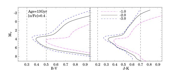
Figure 5: Theoretical isochrones from Demarque et al. (2004), based on the Yonsei-Yale isochrones Version 2 (Yi et al. 2001; Demarque et al. 2004), with parameters shown in the left panel; the dash-dotted, solid, and dotted lines correspond to $\mbox{[Fe/H]}={-1.0}$, $-2.0$, and $-3.0$, respectively. The color ranges of the HES turnoff sample are indicated by the vertical dashed lines.

As pointed out in Paper V, for a magnitude-limited survey the relative survey volume explored by the observed stars differs with the stars’ metallicities, which could also be readily inferred from Figure 5. Besides, as described in Section 2 and Table 1, the HES follow-up procedure is basically a metallicity-biased survey, which favors candidates with lower metallicities. Thus it is interesting to investigate to what extent this effect could impact our sample and the resulting derived MDF. Moreover, we aim at deriving a corrected MDF that is metallicity/volume- unbiased suitable for the comparison with other observational results and theoretical models.

The basic idea of this correction is to derive the survey volume for stars with different metallicities, referenced to a specific metallicity. Here we adopt $\mbox{[Fe/H]}={-2.0}$, because it is near the peak $\mathrm{[Fe/H]}$ of our sample, and also close to the metallicity above which we expect the observed MDF to deviate from the “true” MDF due to metallicity selection bias. It is thus convenient for later comparisons (the choice of a different reference $\mathrm{[Fe/H]}$  will not strongly affect the relative fraction of each $\mathrm{[Fe/H]}$ bin of the corrected MDF). Based on the definition of the survey volume, the corrected volume referenced to $\mbox{[Fe/H]}={-2.0}$ in a specific $(B-V)_{0}$ bin can be directly estimated from $V=10^{0.6(M_{\mathrm{V}}(ref)-M_{\mathrm{V}})}$. As for the turnoff sample, stars within a $(B-V)_{0}$ and $\mathrm{[Fe/H]}$ bin could be either a MSTO star or a subgiant, which obviously explore different survey volumes. Therefore, another step in the correction is used to estimate the ratio of the MSTO stars to subgiants in the sample. Using the luminosity functions from the $Y^{2}$ isochrones and assuming an IMF slope of $x=1.35$ (Salpeter index), for any specific $\mathrm{[Fe/H]}$ and $(B-V)_{0}$we can obtain the number of stars per cubic parsec per absolute magnitude interval for both the MSTO and subgiant branches. Hence a relative density ratio of MSTO stars versus subgiants for the sample is obtained. Given the relative number of MSTO stars and subgiants in each $\mathrm{[Fe/H]}$ and $(B-V)_{0}$ bin, we can then obtain the corrected number of stars within a specific $\mathrm{[Fe/H]}$ and $(B-V)_{0}$ bin by combining the volume and the fraction corresponding to the MSTO and subgiant stars.

Based on this procedure, we derive the volume-corrected MDF of the sample and compare it with the observed one. This is shown in the left panel of Figure 6. As can be seen from inspection of this figure, the survey-volume correction only very slightly affects the shape of the MDF. It mildly decreases the fraction of lower metallicity stars (referenced to $\mbox{[Fe/H]}={-2.0}$) while slightly increasing the fraction at higher metallicity. This is not unexpected because our sample of turnoff stars occupy a relatively narrow range of $(B-V)_{0}$ near the blue end of the isochrones (see Figure 5). Thus, their relative observational volumes for different metallicities or different branches on the isochrones (MSTO or subgiant) do not greatly differ. This is also supported by the spatial distribution of our sample shown in Figure 2. The correction factors of each $\mathrm{[Fe/H]}$ bin for the MDF are listed in the third column of Table 3, and are also applied to the corresponding $\mathrm{[Fe/H]}$ bins of the scaled MDF of the complete candidate sample of 3833 stars derived in Section 3.3 (given in the last column of Table 3).

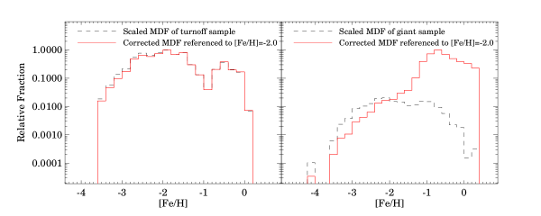
Figure 6: Comparison of the observed and the survey-volume-corrected MDF, shown with the dashed and the solid histograms, respectively. The left panel shows the HES MSTO sample, while the right panel shows the HES giant sample.

Table 3: The survey-volume correction for the observed HES turnoff MDF. The second column refers to the fraction of the scaled MDF; the third column refers to the factor arising from the survey-volume effect as described in Section 3.5, and the last column refers to the corrected fraction for each $\mathrm{[Fe/H]}$ bin.

$\mathrm{[Fe/H]}$	Fraction0	Factor	Fraction
$-$3.50	0.019	0.850	0.016
$-$3.30	0.059	0.790	0.047
$-$3.10	0.140	0.697	0.099
$-$2.90	0.215	0.799	0.174
$-$2.70	0.564	0.847	0.484
$-$2.50	0.770	0.845	0.659
$-$2.30	0.642	0.906	0.589
$-$2.10	0.788	0.937	0.747
$-$1.90	1.000	0.987	1.000
$-$1.70	0.679	1.005	0.691
$-$1.50	0.782	1.023	0.810
$-$1.30	0.306	0.970	0.300
$-$1.10	0.132	0.993	0.133
$-$0.90	0.039	0.999	0.039
$-$0.70	0.205	1.000	0.208
$-$0.50	0.367	1.027	0.382
$-$0.30	0.203	0.965	0.199
$-$0.10	0.164	1.022	0.170
0.10	0.007	1.069	0.007

To further investigate the effect of the survey-volume adjustment on the MDF, the correction procedure was also applied to the metal-poor giant sample of Paper V. A similar method was adopted, except that we assumed that the sample of Paper V are only giants. The corrected MDF is then compared with the observed one, as shown in the right panel of Figure 6. The survey volume effect estimated with our method notably revises the shape of the giants’ MDF. It clearly decreases the fraction of the metal-poor component and dramatically increases the proportion of the relatively metal-rich part. This effect could also be expected from inspection of Figure 5, because within a certain $(B-V)_{0}$ bin the survey volume explored by giants with $\mbox{[Fe/H]}={-3.0}$ (when referenced to $\mbox{[Fe/H]}={-2.0}$) is obviously larger than that of giants with $\mbox{[Fe/H]}={-1.0}$, resulting in a much smaller correction for more metal-deficient giants. Thus, we conclude that although different survey volumes for stars with different metallicities do not affect the observed metallicity distribution of a turnoff-star dominated sample, they will obviously change the observed MDF of a giant-dominated sample, and cannot be ignored. In Table 4, we list the correction factors for each $\mathrm{[Fe/H]}$ bin of the giants’ MDF, and applied the values to corresponding bins of the scaled MDF of Paper V.

Table 4: The correction factor arising from the survey-volume effect for corresponding $\mathrm{[Fe/H]}$ bins of the observed giant MDF, as described in Section 3.5

[Fe/H]	$-4.00$	$-3.50$	$-3.30$	$-3.10$	$-2.90$	$-2.70$	$-2.50$	$-2.30$	$-2.10$	$-1.90$	$-1.70$
Factor	0.330	0.331	0.327	0.287	0.341	0.407	0.499	0.698	0.834	1.184	2.048
[Fe/H]	$-1.50$	$-1.30$	$-1.10$	$-0.90$	$-0.70$	$-0.50$	$-0.30$	$-0.10$	$0.10$	$0.30$
Factor	3.491	9.003	24.97	48.22	107.3	121.9	219.0	211.9	2132.	738.4

3.6 Comparison with the giants’ MDF

The MDF of the HES MSTO sample can now be compared with that of the giants from Paper V, as shown in Figure 7. The comparison between the two MDFs can be considered in two parts.

First, at the metal-poor end with $\mbox{[Fe/H]}<{-2.0}$ (exclusive of the ultra metal-poor component with $\mbox{[Fe/H]}<{-4.0}$ of Paper V), both MDFs agree on the dramatic decrease of stars below $\mbox{[Fe/H]}<{-3.0}$ and the sharp drop at $\mbox{[Fe/H]}\sim{-3.6}$. Besides, a $\chi^{2}$-test of the null hypothesis that the two samples are drawn from the same parent distribution yields a probability of $\sim 1$. This indicates that the two samples present are quite analogous distributions in this metallicity region. This is not unexpected because both the turnoff and giant samples were aimed to sample the Galactic halo population and were selected with similar criteria in order to derive a statistically complete sample for metal-poor stars. Thus, the two samples should follow similar statistical properties in the metallicity region where the halo population dominates.

The two MDFs notably differ from each other in the fraction of the relatively metal-rich component (e.g., $\mbox{[Fe/H]}>{-2.0}$), with the giant MDF revealing a higher fraction. For MDFs in the region with $\mbox{[Fe/H]}>{-2.0}$, the $\chi^{2}$-test yields a probability of $\sim 0$, suggesting very different distributions. This is not difficult to understand. As shown in the previous section, the correction on the survey-volume has very different effects on the two MDFs. Also, the cutoff at $(B-V)_{0}$$=0.5$ leads to a cutoff at comparatively lower metallicites for the turnoff MDF. Hence, the two samples present rather distinct MDFs in this region. However, one should keep in mind that the size of the subgroup of candidates with least possibility of being metal-poor, i.e., mpcc, in our turnoff sample is very limited (only 16 “accepted” stars), and was biased against in the whole selection and observation procedure. Consequently, it may be incomplete for a thorough statistical comparison of MDFs in this $\mathrm{[Fe/H]}$ region.

Therefore, as the primary motivation of this work is to discuss the properties of the halo MDF, the completeness of both the turnoff and giant samples and the above quantitative investigation should be reliable in the metallicity region which is of greatest interest ($\mbox{[Fe/H]}<{-2.0}$, especially the metal-deficient tail between $\mbox{[Fe/H]}<{-2.5}$ and $-3.6$). The reader should note that the low-metallicity tail discussed in this work is different from that discussed in Paper V which extends to $\mbox{[Fe/H]}<{-4.0}$.

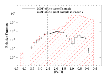
Figure 7: The observed MDF of HES MSTO stars (open histogram with solid line) is compared with that of giants by Paper V (filled histogram with dashed line). A relative normalization which scaled the maximum fraction to 1.0 is used for MDFs here and throughout the paper. Note that the two MDFs are scaled to match at $\mbox{[Fe/H]}={-2.5}$ (the starting point of the metal-deficient tail we defined, and also marked out with the vertical dashed line).

4 Do Theoretical Predictions Fit the Observations?

One of the crucial roles that the observed halo MDF plays is to examine and constrain theoretical models of Galactic chemical evolution. In order to carry out such a comparison with any theoretical predictions, we first need to convert the theoretical MDFs into a form that corresponds to what would be observed in a survey with the same observational strategy and selection criteria as for the HES turnoff sample.

The first modification of the theoretical MDFs is to account for the HES selection function. To accomplish this, we inverted the calibration of Beers et al. (1999) to convert each $\mathrm{[Fe/H]}$ into a pair of $(B-V)_{0}$ and KP or $(J-K)_{0}$ and KP. Considering the fact that the selection function varies with $(B-V)_{0}$ or $(J-K)_{0}$ (see Paper IV, V, and Section 3.4), these theoretical “stars” were selected to follow the distribution of $(B-V)_{0}$ and $(J-K)_{0}$ of our observed sample. Following this, random Gaussian errors with standard deviations to reflect those in the measured $(B-V)_{0}$ and $(J-K)_{0}$  color, and the KP index were computed and added ($\sigma_{B-V}$=0.06, $\sigma_{J-K}$=0.1, and $\sigma_{KP}$=1.0). Finally, we applied the same criteria for $(B-V)_{0}$ or $(J-K)_{0}$ versus KP to select metal-poor “candidates” from these theoretical stars. Using the above procedure we obtain a model MDF as it would have been observed in the HES (which we refer to as “as observed”). We compare it with the observed MDF of the turnoff sample in the following discussions. Since the low-metallicity tail of the MDF is of the greatest interest to this study, the following discussion will focus on the comparisons in the metallicity region between $\mbox{[Fe/H]}={-2.0}$ and $-3.6$ (where the observed MDF is considered statistically reliable).

4.1 Theoretical predictions based on the Simple Model

We begin our observational-theoretical comparison with the Simple Model (Searle & Sargent 1972; Pagel & Patchett 1975) of Galactic chemical evolution. It describes the basic form of a closed system which evolves from initially zero-metallicity gas and remains chemically homogeneous at all times. Hartwick (1976) extended this model such that star formation ends once the gas is either consumed or removed (essentially relaxing the closure requirement of the system). Here we make use of this model as parameterized by the effective yield, $y_{\mbox{\scriptsize eff}}$, and adopting the same value as in Paper V, log₁₀ $y_{\mbox{\scriptsize eff}}=-1.7$.

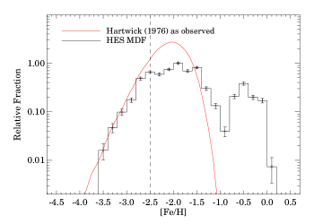
Figure 8: The HES MSTO MDF (black histogram) is compared with that predicted by Hartwick (1976)’s modified Simple Model (1og₁₀ $y_{\mbox{\scriptsize eff}}=-1.7$) as it would have been observed in the HES (red solid line). Note that for all the comparisons that follow that we have scaled the model MDFs in such a way that they could best fit the metal-poor tail of the observed MDF. The vertical dashed line refers to $\mbox{[Fe/H]}={-2.5}$ here and in the following plots too.

The result is shown in Figure 8. As can be seen, the mass-loss modified Simple Model is able to fit the position ($\mbox{[Fe/H]}\sim{-2.0}$) but not the height of the peak. It does, however, well fit the general shape of MDF tail with $\mathrm{[Fe/H]}$ from $-2.7$ through $-3.6$, although it can only predict a smooth drop of the metal-poor tail at $\mbox{[Fe/H]}\sim{-3.6}$. This is not entirely unexpected considering the fact that the real Galactic halo(s) could certainly be more complicated than a simple one-zone model assuming the Instantaneous Recycling Approximation (IRA – Tinsley 1980).

Prantzos (2003) addressed the effect of the IRA in the determination of the MDF of a system such as the Milky Way and suggested a physically motivated modification to the simple outflow model, i.e., a composite model adopting a relaxed IRA, and assuming both early infall and outflow to solve the so-called “G dwarf problem”. Based on this model, and the further accumulation of observational data, Prantzos (2008) presented a semi-analytical model in the framework of the hierarchical merging paradigm for structure formation which assumes that the Galactic halo is composed of the stellar debris of several sub-halos following either the observed properties of dwarf galaxies or a structure formation calculation.

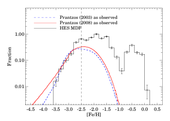
Figure 9: Comparison of the HES MSTO MDF and the models of Prantzos (2003) (dashed line) and Prantzos (2008) (solid line).

As shown in Figure 9, both the composite model with an early phase of gas infall by Prantzos (2003) and the hierarchical merging scenario for the formation by Prantzos (2008) fit the shape of the observed MDF tail between $-2.9$ and $-3.4$ rather well. However, the location of the peak of the MDF is not correctly predicted in either case and neither of them reproduces the sharp drop at $\mbox{[Fe/H]}\sim{-3.6}$. Rather, they predict a smooth decrease of numbers of EMP stars which extend to $\mbox{[Fe/H]}<{-4.0}$.

4.2 Other theoretical predictions

Besides models based on variations of the chemical evolution scheme of the Simple Model, there are quite a number of other models based on theoretical analyses or simulations. Here we compare our observation with two such theoretical predictions.

The first considered is the model of Karlsson (2006) which focuses on the metal-poor tail with $\mbox{[Fe/H]}\leq{-3.0}$, and attempts to explain the “gap” in the halo MDF with $\mathrm{[Fe/H]}$ between $-4.0$ and $-5.0$. It adoptes a scenario of negative feedback from Population III stars. Figure 10 suggests that it only roughly fits the portion of the MDF with $\mbox{[Fe/H]}<{-3.0}$. It also fails to predict the sharp drop at the low-metallicity end as well.

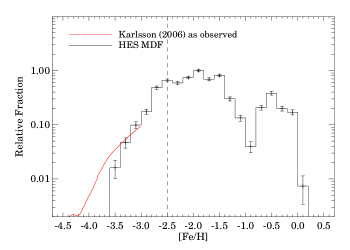
Figure 10: Comparison of the HES MSTO MDF and the model of (Karlsson 2006).

Another model that has been tested is GAlaxy MErger Tree and Evolution (GAMETE – Salvadori et al. 2007). It is a Monte Carlo code to reconstruct the merger tree of the Milky Way and to follow the evolution of gas and stars along the tree. This model defines an input parameter, the critical metallicity $Z_{cr}$, which governs the transition from Pop III to Pop II star formation. We compare our observed MDF with the simulated results corresponding to different values of $Z_{cr}$, as shown in Figure 11. Although according to the observational data available at that time, $Z_{cr}=10^{-4}Z_{\odot}$ was regarded as the fiducial model, it obviously cannot fit our observations here. All the predictions fail to fit the location of the peak of the observed MDF. Similarly to the conclusions in Paper V, the model with $Z_{cr}=10^{-3.4}Z_{\odot}$ appears to partially fit our observed MDF, being able to reproduce the tail with $\mbox{[Fe/H]}<{-3.0}$ and best predict the sharp drop at $\mbox{[Fe/H]}\sim{-3.6}$.

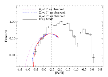
Figure 11: Comparison of the HES MDF and the model of Salvadori et al. (2007). The purple dashed, blue dash-dotted, and red solid lines correspond to models with $Z_{cr}=10^{-4}Z_{\odot}$, $10^{-3.5}Z_{\odot}$, and $10^{-3.4}Z_{\odot}$, respectively.

5 Summary and Discussions

Based on the (for now) largest metal-poor turnoff-star sample from the HES database and moderate-resolution follow-up observations, we have statistically investigated the MDF of local MSTO stars in the Galactic halo.

1. With reference to $\mbox{[Fe/H]}={-2.0}$, the effects of relative survey volumes have been quantitatively estimated based on theoretical isochrones and applied to the observed MDFs of both the HES turnoff and giants samples. It is shown that the survey-volume effect does not substantially alter the turnoff MDF while it dramatically changes the MDF of the giant sample from Paper V.

2. The survey-volume corrected and metal-poor-class scaled MDFs of the turnoff sample has been compared with that of the halo giants. Though the two MDFs notably differ in the region with $\mbox{[Fe/H]}>{-2.0}$ (where our sample starts to be incomplete), for the metal-deficient region (e.g., $\mbox{[Fe/H]}<{-2.0}$) the $\chi^{2}$-test suggests that the two MDFs are quite similar. Furthermore, both MDFs agree regarding the sharp drop at $\mbox{[Fe/H]}\sim{-3.6}$. Hence, for an MDF dominated by the halo population, the two MDFs agree well.

3. Theoretical models of Galactic chemical evolution have been discussed. They can only fit portions of the observed MSTO MDF while none of them fully reproduces the features of the observations. In particular, they fail to simultaneously fit the peak and the metal-deficient tail between $\mbox{[Fe/H]}\sim{-2.5}$ to $-3.6$. Although the $Z_{cr}=10^{-3.4}Z_{\odot}$ case of the Salvadori et al. (2007) model can only partially fit the observed MDF it is able to best predict the sharp drop at $\mbox{[Fe/H]}\sim{-3.6}$.

4. Generally, both selection criteria using KP plus $(B-V)_{0}$ and $(J-K)_{0}$ serve as efficient selectors of metal-poor stars. They are capable to reach a selection fraction up to 100% for the EMP candidates of our sample.

Considering the fact that our sample mainly consists of unevolved main-sequence (and subgiant) stars with low metallicities, it could also provide additional useful information on Galactic chemical evolution. For example, a kinematic analysis of this sample could be used to re-visit the role of accretion of the interstellar medium during the long lifetimes of metal-poor stars, as approximately calculated in a number of early works (e.g., Talbot & Newman 1977; Yoshii 1981; Iben 1983) and also discussed by more recent studies (e.g, Christlieb et al. 2004; Norris et al. 2007; Frebel et al. 2009).

It should also be pointed out that all of our comparisons of the MDFs have been performed under the assumption that we are modeling a single halo population, which current evidence suggests is an over-simplification. It seems likely that the observed MDFs for both the HES MSTO stars and the HES giants comprise overlapping contributions from the outer-halo population at the lowest metallicities and the inner halo at intermediate low metallicities, with respective tails of as-yet unknown relative strengths and convolved with the HES metallicity selection bias that becomes more severe above $\mbox{[Fe/H]}\sim{-2.5}$ to $-2.0$. This possibility was already mentioned in Paper V where it was noted that there appeared to be relatively larger fractions of EMP stars at heights above the plane $|$Z$|$ $>$ 15 kpc than in the intermediate range 5 $<$ $|$Z$|$ $<$ 15 kpc. This is in line with the expectations of the dual halo interpretation of Carollo et al. (2007, 2010). Progress on this issue will come from consideration of the dual halo modeling approach, ideally in combination with a full kinematic analysis of these samples that forms the basis of a paper in preparation.

However, the HES metal-poor turnoff sample discussed in this paper contains no objects with $\mbox{[Fe/H]}<{-3.6}$ which obviously do exist. Thus, we are not able to discuss the performance of theoretical MDFs in the most metal-deficient regime. Larger statistically complete samples are required for a thorough comparison with theoretical predictions. Fortunately, such samples will be obtained from much larger and deeper surveys in the near future, such as from SEGUE-2 and the Apache POint Galactic Evolution Experiment (APOGEE), the Large Sky Area Multi-Object Fiber Spectroscopic Telescope (LAMOST, Zhao et al. 2006), and the Southern Sky Survey (Keller et al. 2007).