Graphical rule of transforming continuous-variable graph states by local homodyne detection

Abstract

Graphical rule, describing that any single-mode homodyne detection turns a given continuous-variable (CV) graph state into a new one, is presented. Employing two simple graphical rules: local complement operation and vertex deletion (single quadrature-amplitude $\hat{x}$ measurement), the graphical rule for any single-mode quadrature component measurement can be obtained. The shape of CV weighted graph state may be designed and constructed easily from a given larger graph state by applying this graphical rule.

Graph states - or equivalently called stabilizer states, are a particularly interesting class of multipartite entangled states associated with graphs one ; two and play several fundamental roles in quantum information such as one-way quantum computation, quantum error correction, multiparty quantum communication, quantum simulation, Bell inequalities theorem, etc.

Continuous variables (CV) are a promising new flavor of quantum information, whose potential is still largely unexplored. CV cluster and graph states have been proposed seven , which can be generated by squeezed state and linear optics seven ; eight or optical frequency comb in an optical parametric oscillator nine , and demonstrated experimentally for the four-mode cluster state ten ; eleven . The one-way CV quantum computation was also proposed with the CV cluster state twelve ; twelve1 ; twelve2 and demonstrated with Gaussian operations experimentally thirteen .

It is well known that Clifford operations or projective measurement associated with operators in the Pauli group can be described by the stabilizer formalism. For example, the action of local Clifford operations on qubit forteen ; one or CV fifteen ; sixteen ; sixteen1 graph states can entirely be understood in terms of a single elementary graph transformation rule, called the local complement rule. Moreover, any measurement of operators in Pauli group turns a given qubit graph state into a new one one ; two . The graphical rule also can describe the effect of Pauli measurement on the qubit graph states. Since CV graph states have many different properties from the qubit, many concepts and methods for qubit can not be extended to CV directly. For example, the CV weighted graph states can be expressed by the stabilizer formalism sixteen . It is distinctively different from the qubit weighted graph states, which can not be expressed by the stabilizer formalism. In this paper, how to graphically describe the effect of local Pauli measurements (local homodyne detection) on the ideal (i.e., infinitely squeezed) CV weighted graph states is investigated.

In order to conveniently describe our results, we briefly review some basic elements of the theory of CV graph states and operations which are needed in this paper seventeen ; seven ; fifteen ; sixteen . The single mode Pauli operators are defined as $X(s)=exp[-is\hat{p}]$ and $Z(t)=exp[it\hat{x}]$, where $s,t\in\mathbb{R}$, $\hat{x}=(\hat{a}+\hat{a}^{\dagger})/\sqrt{2}$ (quadrature-amplitude or position) and $\hat{p}=-i(\hat{a}-\hat{a}^{\dagger})/\sqrt{2}$ (quadrature-phase or momentum). The Pauli operator $X(s)$ is a position-translation operator, which acts on the computational basis of position eigenstates as $X(s)|q\rangle=|q+s\rangle$, whereas $Z$ is a momentum-translation operator, which acts on the momentum eigenstates as $Z(t)|p\rangle=|p+t\rangle$. The Pauli operators for one mode can be used to construct a set of Pauli operators $\{X_{i}(s_{i}),Z_{i}(t_{i});i=1,...,n\}$ for n-mode systems. This set generates the Pauli group $\mathcal{C}_{1}$. For $k\geq 2$, we can recursively define $\mathcal{C}_{k}$ as eighteen

$$\mathcal{C}_{k}=\{U|U\mathcal{C}_{1}U^{\dagger}\subseteq\mathcal{C}_{k-1}\}.$$ (1)

For every $k$, $\mathcal{C}_{k}\supset\mathcal{C}_{k-1}$, and the set difference $\mathcal{C}_{k}/\mathcal{C}_{k-1}$ is nonempty.

$\mathcal{C}_{2}$ is a group called the Clifford group, which is the normalizer of the Pauli group, whose transformations acting by conjugating, preserve the Pauli group. The Clifford group $\mathcal{C}_{2}$ for CV is shown eighteen to be the (semidirect) product of the Pauli group and linear symplectic group of all one-mode and two-mode squeezing transformations. Transformation between the position and momentum basis is given by the Fourier transform operator $F=exp[i(\pi/4)(\hat{x}^{2}+\hat{p}^{2})]$, with $F|q\rangle_{x}=|q\rangle_{p}$. This is the generalization of the Hadamard gate for qubits. The phase gate $P(\eta)=exp[i(\eta/2)\hat{x}^{2}]$ with $\eta\in\mathbb{R}$ is a squeezing operation for CV and the action $P(\eta)RP^{-1}(\eta)$ on the Pauli operators is

$$P(\eta):X(s) \rightarrow e^{-is^{2}\eta/2}Z(s\eta)X(s),$$

$$Z(t) \rightarrow Z(t),$$ (2)

in analogy to the phase gate of qubit. The controlled operation C-Z is generalized to controlled-$Z(C_{Z})$. This gate $C_{Z}=exp[i\hat{x}_{1}\bigotimes\hat{x}_{2}]$ provides the basic interaction for two mode 1 and 2, and describes the quantum nondemolition (QND) interaction. This set $\{X(s),F,P(\eta),C-Z;s,\eta\in\mathbb{R}\}$ generates the Clifford group. Here the controlled operation with any interaction strength $C_{Z}(\Omega)=exp[i\Omega\hat{x}_{1}\bigotimes\hat{x}_{2}]$ ($\Omega\in\mathbb{R}$) will be used in this paper. Another type of the phase gate will also be utilized $P_{X}(\eta)=FP(\eta)F^{-1}=exp[i(\eta/2)\hat{p}^{2}]$ and the action on the Pauli operators is

$$P_{X}(\eta):X(s) \rightarrow X(s),$$

$$Z(t) \rightarrow e^{-it^{2}\eta/2}X(-t\eta)Z(t),$$ (3)

where $P_{X}(\eta)^{\dagger}=P_{X}(\eta)^{-1}=P_{X}(-\eta)$.

A weighted graph quantum state is described by a mathematical graph $G=(V,E)$, i.e. a finite set of $n$ vertices $V$ connected by a set of edges $E$ forteen , in which every edge is specified by a factor $\Omega_{ab}$ corresponding to the strength the modes a and b. The preparation procedure of CV weighted graph states is only to use the Clifford operations: first, prepare each mode (or graph vertex) in a phase-squeezed state, approximating a zero-phase eigenstate (analog of Pauli-X eigenstates), then, apply the QND coupling ($C_{Z}(\Omega)$) with the different interaction strength $\Omega_{jk}$ to each pair of modes $(j,k)$ linked by a weighted edge in the graph. The CV unweighted graph states is to use the QND interaction all with the same strength. Since all C-Z gates commute, the resulting CV graph state becomes, in the limit of infinite squeezing, $g_{a}=(\hat{p}_{a}-\sum_{b\in N_{a}}\Omega_{ab}\hat{x}_{b})\rightarrow 0$, where the modes $a\in V$ correspond to the vertices of the graph of $n$ modes, while the modes $b\in N_{a}$ are the nearest neighbors of mode $a$. This relation is as a simultaneous zero-eigenstate of the position-momentum linear combination operators. The corresponding $n$ independent stabilizers for CV weighted graph states are expressed by $G_{a}(\xi)=exp[-i\xi g_{a}]=X_{a}(\xi)\prod_{b\in N_{a}}Z_{b}(\Omega_{ab}\xi)$ with $\xi\in\mathbb{R}$.

The local complement operation on vertex $a$ of CV weighted graph state is expressed by sixteen

$$U_{LG_{a}}(\delta)=P_{Xa}(-\delta)\prod_{b\in N_{a}}P_{b}(\Omega_{ab}^{2}\delta).$$ (4)

The action of this local complement operation on CV weighted graph states can be stated in purely graph theoretical terms, which completely characterize the evolution of CV weighted graph states under this local complement operation. The graph rule of applying this local complement operation on vertex $a$ is described as: first obtain the subgraph of $G$ generated by the neighborhood $N_{a}$ of $a$, then reset the weight factor of all edges of this subgraph calculated with the equation $\Omega_{b_{i}b_{j}}^{\prime}=\Omega_{b_{i}b_{j}}-\Omega_{ab_{i}}\Omega_{ab_{j}}\delta$, at last delete all the edges with the weight factor of zero, and leave the rest of the graph unchanged. Here, a subgraph $G[C]$ of a graph $G=(V,E)$, where $C\subset V$, is obtained by deleting all vertices and the incident edges that are not contained in $C$.

First, we consider the simplest case of the quadrature-amplitude ($\hat{x}$) component measurement on vertex $a$ of CV weighted graph state. After the $\hat{x}$ component measurement on vertex $a$ with the result $x_{a}$ by local homodyne detection, a CV weighted graph state $|G\rangle$ will transform into another weighted graph state $|G^{\prime}\rangle=U_{x_{a}}^{(a)}|G-a\rangle$, where $G-a$ denote the graph that is obtained from $G$ by deleting the vertex $a$ and all edges incident with $a$, and

$$U_{x_{a}}^{(a)}=\prod_{b\in N_{a}}Z^{(b)}(x_{a}).$$ (5)

Thus, in case of a measurement of quadrature-amplitude ($\hat{x}$), the resulting graph can be produced by simply deleting the measured vertex $a$ and related edges from the graph, then translating the measurement result into the momentum component of the neighborhood vertices $N_{a}$ of $a$. Based on above two simple graphical rules: local complement operation and the single quadrature-amplitude $\hat{x}$ measurement (also called vertex deletion), the graphical rules for any quadrature component measurement can be obtained as the following.

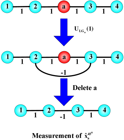
Figure 1: Example of a $\hat{x}^{45^{0}}$ measurement on vertex a in a linear cluster.

Any quadrature component of an optical mode is expressed by

$$\hat{x}^{\theta} = (\hat{a}e^{-i\theta}+\hat{a}^{\dagger}e^{i\theta})/\sqrt{2}$$ (6)

$$= \cos\theta\hat{x}+\sin\theta\hat{p}.$$

The basic idea of obtaining the graphical rules for any quadrature component measurement is that, first transform the quadrature-amplitude $\hat{x}$ of vertex $a$ into the measured component $\hat{x}^{\prime}=\cos\theta\hat{x}+\sin\theta\hat{p}$ by local Gaussian operations, then perform single quadrature-amplitude $\hat{x}$ measurement (vertex deletion). Now we first apply local complement operation $U_{LG_{a}}(\delta)$ on vertex $a$ of CV weighted graph state. Thus the quadrature-amplitude of vertex $a$ is transformed into $\hat{x}_{a}^{\prime}=\hat{x}_{a}+\delta\hat{p}_{a}$, where $\delta=\tan\theta$. Then we perform the quadrature-amplitude measurement on vertex $a$ with the detection result $x_{a}^{\prime}$. The new graph is obtained by deleting the measured vertex $a$ and related edges from the graph, then translating the measurement result $x_{a}^{\prime}$ into the momentum component of the neighborhood vertices $N_{a}$ of $a$. The new graph can be expressed by $|G^{\prime\prime}\rangle=U_{x^{\prime}_{a}}^{(a)}|G^{\prime}-a\rangle$ and $|G^{\prime}\rangle=U_{LG_{a}}(\tan\theta)|G\rangle$. Figure 1 presents an example of a $\hat{x}^{45^{0}}$ measurement on a linear cluster, which removes the measured mode and still keeps the neighbor vertices to be joined.

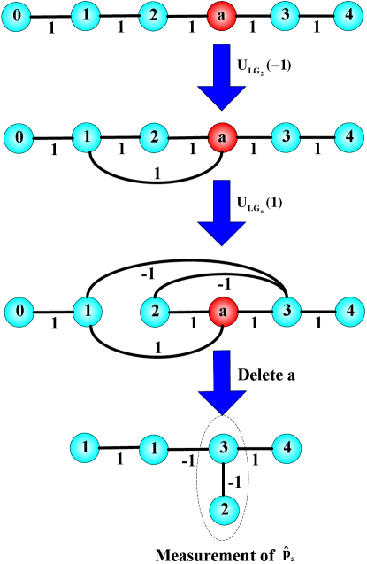
Figure 2: Example of a $\hat{p}$ measurement on vertex a on a linear cluster. The vertex 2 was chosen as the special neighbor $b_{0}$.

Now considering the single quadrature-phase $\hat{p}$ measurement, it requires that $\delta$ approach infinite for local complement operation $U_{LG_{a}}(\delta)$ on vertex $a$. Apparently it is impractical. So we consider the different local operations to obtain the graphical rule for quadrature-phase component measurement. First, chooses any of neighbor vertex $b$ of vertex $a$, and applies local complement operation $U_{LG_{b}}(-1/\Omega_{ab}^{2})$ on vertex $b$. Then applies local local complement operation $U_{LG_{a}}(1)$ on vertex $a$. Thus the quadrature-amplitude and phase of vertex $a$ are transformed into $\hat{x}_{a}^{\prime}=\hat{p}_{a}$, $\hat{p}_{a}^{\prime}=\hat{p}_{a}-\hat{x}_{a}$ by $P_{Xa}(-1)P_{a}(-1)$. The new graph can be expressed by $|G^{\prime\prime}\rangle=U_{x^{\prime}_{a}}^{(a)}|G^{\prime}-a\rangle$ and $|G^{\prime}\rangle=U_{LG_{a}}(1)U_{LG_{b}}(-1/\Omega_{ab}^{2})|G\rangle$. An example of a $\hat{p}$ measurement on a linear cluster is depicted in Fig. 2. It is easy to see that two adjacent vertices combine into a single vertex with the bonds attached to each. Figure 3 presents a $\hat{p}$ measurement on a complex weighted graph state.

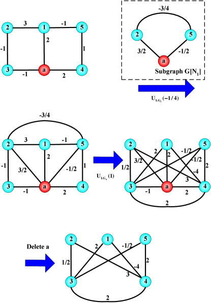
Figure 3: The graphical rule for a $\hat{p}$ measurement on a complex weighted graph state. The vertex 1 was chosen as the special neighbor $b_{0}$.

In summary, graphical rule of transforming ideal CV weighted graph state by any single-mode homodyne detection is described. The graphical rule for any single-mode quadrature component measurement is obtained by two simple graphic rules: local complement operation and vertex deletion. This work will be very helpful to specify which graph states can mapped by the single-mode homodyne detection and to apply in one-way CV quantum computation.

^†Corresponding author’s email address: jzhang74@sxu.edu.cn, jzhang74@yahoo.com

I ACKNOWLEDGMENTS

This research was supported in part by NSFC for Distinguished Young Scholars (Grant No. 10725416), National Basic Research Program of China (Grant No. 2006CB921101, 2011CB921601), NSFC Project for Excellent Research Team (Grant No. 60821004), and Program for the Top Young and Middle-aged Innovative Talents of Higher Learning Institutions of Shanxi.

$Note$ $added.$ - Right after completion of this work, another work appeared ninteen , where two simple and special local homodyne measurements were investigated experimentally.

References

- (1) M. Hein, et al., Phys. Rev. A 69, 062311 (2004).
- (2) M. Hein, et al., quant-ph/0602096.
- (3) J. Zhang, S. L. Braunstein, Phys. Rev. A 73, 032318 (2006).
- (4) P. van Loock, C. Weedbrook and M. Gu, Phys. Rev. A 76, 032321 (2007).
- (5) N. C. Menicucci, S. T. Flammia, H. Zaidi, and O. Pfister, Phys. Rev. A 76, 010302(R) (2007); N. C. Menicucci, S. T. Flammia, and O. Pfister, Phys. Rev. Lett. 101, 130501 (2008).
- (6) X. Su, A. Tan, X Jia, J. Zhang, C. Xie, and K. Peng, Phys. Rev. Lett. 98, 070502 (2007).
- (7) M. Yukawa, R. Ukai, P. van Loock, and A. Furusawa, Phys. Rev. A 78, 012301 (2008).
- (8) N. C. Menicucci et al., Phys. Rev. Lett. 97, 110501 (2006).
- (9) P. van Loock, J. Opt. Soc. Am. B 24, 340 (2007).
- (10) M. Gu, C. Weedbrook, N. C. Menicucci, T. C. Ralph, P. van Loock, Phys. Rev. A 79, 062318 (2009).
- (11) Y. Miwa, J. I. Yoshikawa, P. van Loock, and A. Furusawa, Phys. Rev. A 80, 050303(R) (2009); Y. Wang, X. Su, H. Shen, A. Tan, C. Xie, and K. Peng, Phys. Rev. A 81, 022311 (2010); R. Ukai, N. Iwata, Y. Shimokawa, S. Armstrong, A. Politi, J. Yoshikawa, P. van Loock, and A. Furusawa, arXiv:1001.4860.
- (12) M. Van den Nest, J. Dehaene, and B. De Moor, Phys. Rev. A 69, 022316 (2004).
- (13) J. Zhang, Phys. Rev. A 78, 034301 (2008).
- (14) J. Zhang, Phys. Rev. A 78, 052307 (2008).
- (15) J. Zhang, G. He, and G. Zeng, Phys. Rev. A 80, 052333 (2009).
- (16) S. D. Bartlett, et al., Phys. Rev. Lett. 88, 097904 (2002).
- (17) X. Zhou, D. W. Leung, I. L. Chuang, Phys. Rev. A 62, 052316 (2000).
- (18) Y. Miwa, R. Ukai, J. Yoshikawa, R. Filip, P. van Loock, and A. Furusawa, arXiv:1006.2225.