Graph-Valued Regression

Abstract

Undirected graphical models encode in a graph $G$ the dependency structure of a random vector $Y$. In many applications, it is of interest to model $Y$ given another random vector $X$ as input. We refer to the problem of estimating the graph $G(x)$ of $Y$ conditioned on $X=x$ as “graph-valued regression.” In this paper, we propose a semiparametric method for estimating $G(x)$ that builds a tree on the $X$ space just as in CART (classification and regression trees), but at each leaf of the tree estimates a graph. We call the method “Graph-optimized CART,” or Go-CART. We study the theoretical properties of Go-CART using dyadic partitioning trees, establishing oracle inequalities on risk minimization and tree partition consistency. We also demonstrate the application of Go-CART to a meteorological dataset, showing how graph-valued regression can provide a useful tool for analyzing complex data.

,  ,  and

1 Introduction

Let $Y$ be a $p$-dimensional random vector with distribution $P$. A common way to study the structure of $P$ is to construct the undirected graph $G=(V,E)$, where the vertex set $V$ corresponds to the $p$ components of the vector $Y$. The edge set $E$ is a subset of the pairs of vertices, where an edge between $Y_{j}$ and $Y_{k}$ is absent if and only if $Y_{j}$ is conditionally independent of $Y_{k}$ given all the other variables. Suppose now that $Y$ and $X$ are both random vectors, and let $P(\cdot{\,|\,}X)$ denote the conditional distribution of $Y$ given $X$. In a typical regression problem, we are interested in the conditional mean $\mu(x)=\mathbb{E}\left(Y{\,|\,}X=x\right)$. But if $Y$ is multivariate, we may also be interested in how the structure of $P(\cdot{\,|\,}X)$ varies as a function of $X$. In particular, let $G(x)$ be the undirected graph corresponding to $P(\cdot{\,|\,}X=x)$. We refer to the problem of estimating $G(x)$ as graph-valued regression.

Let ${\cal G}=\{G(x):\ x\in{\cal X}\}$ be a set of graphs indexed by $x\in\mathcal{X}$, where ${\cal X}$ is the domain of $X$. Then ${\cal G}$ induces a partition of ${\cal X}$, denoted as ${\cal X}_{1},\ldots,{\cal X}_{m}$, where $x_{1}$ and $x_{2}$ lie in the same partition element if and only if $G(x_{1})=G(x_{2})$. Graph-valued regression is thus the problem of estimating the partition and estimating the graph within each partition element.

We present three different partition-based graph estimators; two that use global optimization, and one based on a greedy splitting procedure. One of the optimization based schemes uses penalized empirical risk minimization; the other uses held-out risk minimization. As we show, both methods enjoy strong theoretical properties under relatively weak assumptions; in particular, we establish oracle inequalities on the excess risk of the estimators, and tree partition consistency (under stronger assumptions) in Section 4. While the optimization based estimates are attractive, they do not scale well computationally when the input dimension is large. An alternative is to adapt the greedy algorithms of classical CART, as we describe in Section 3.3. In Section 5 we present experimental results on both synthetic data and a meteorological dataset, demonstrating how graph-valued regression can be an effective tool for analyzing high dimensional data with covariates.

2 Graph-Valued Regression

Let $y_{1},\ldots,y_{n}$ be a random sample of vectors from $P$, where each $y_{i}\in{\mathbb{R}}^{p}$. We are interested in the case where $p$ is large and, in fact, may diverge with $n$ asymptotically. One way to estimate $G$ from the sample is the graphical lasso or glasso (Yuan and Lin, 2007; Friedman, Hastie and Tibshirani, 2007; Banerjee, Ghaoui and d’Aspremont, 2008), where one assumes that $P$ is Gaussian with mean $\mu$ and covariance matrix $\Sigma$. Missing edges in the graph correspond to zero elements in the precision matrix $\Omega=\Sigma^{-1}$ (Whittaker, 1990; Edwards, 1995; Lauritzen, 1996). A sparse estimate of $\Omega$ is obtained by solving

$$\widehat{\Omega}=\mathop{\text{\rm arg\,min}}_{\Omega\succ 0}\bigl{\{}{\rm tr}(S\Omega)-\log|\Omega|+\lambda\|\Omega\|_{1}\bigr{\}}$$ (2.1)

where $\Omega$ is positive definite, $S$ is the sample covariance matrix, and $\|\Omega\|_{1}=\sum_{j,k}|\Omega_{jk}|$ is the elementwise $\ell_{1}$-norm of $\Omega$. Friedman, Hastie and Tibshirani (2007) develop a efficient algorithm for finding $\widehat{\Omega}$ that involves estimating a single row (and column) of $\Omega$ in each iteration by solving a lasso regression. The theoretical properties of $\widehat{\Omega}$ have been studied by Rothman et al. (2008) and Ravikumar et al. (2009). In practice, it seems that the glasso yields reasonable graph estimators even if $Y$ is not Gaussian; however, proving conditions under which this happens is an open problem.

We briefly mention three different strategies for estimating $G(x)$, the graph of $Y$ conditioned on $X=x$, each of which builds upon the glasso.

Parametric Estimators. Assume that $Z=(X,Y)$ is jointly multivariate Gaussian with covariance matrix

$$\Sigma=\left(\begin{array}[]{cc}\Sigma_{X}&\Sigma_{XY}\\ \Sigma_{YX}&\Sigma_{Y}\\ \end{array}\right).$$

We can estimate $\Sigma_{X}$, $\Sigma_{Y}$, and $\Sigma_{XY}$ by their corresponding sample quantities $\widehat{\Sigma}_{X}$, $\widehat{\Sigma}_{Y}$, and $\widehat{\Sigma}_{XY}$, and the marginal precision matrix of $X$, denoted as $\Omega_{X}$, can be estimated using the glasso. The conditional distribution of $Y$ given $X=x$ is obtained by standard Gaussian formulas. In particular, the conditional covariance matrix of $Y{\,|\,}X$ is $\widehat{\Sigma}_{Y|X}=\widehat{\Sigma}_{Y}-\widehat{\Sigma}_{YX}\widehat{\Omega}_{X}\widehat{\Sigma}_{XY}$ and a sparse estimate of $\widehat{\Omega}_{Y|X}$ can be obtained by directly plugging $\widehat{\Sigma}_{Y|X}$ into glasso. However, the estimated graph does not vary with different values of $X$.

Kernel Smoothing Estimators. We assume that $Y$ given $X$ is Gaussian, but without making any assumption about the marginal distribution of $X$. Thus $Y{\,|\,}X=x\sim N(\mu(x),\Sigma(x))$. Under the assumption that both $\mu(x)$ and $\Sigma(x)$ are smooth functions of $x$, we estimate $\Sigma(x)$ via kernel smoothing:

$$\widehat{\Sigma}(x)=\sum_{i=1}^{n}K\left(\frac{\|x-x_{i}\|}{h}\right)\left(y_{i}-\widehat{\mu}(x)\right)\left(y_{i}-\widehat{\mu}(x)\right)^{T}\Bigm{/}{\sum_{i=1}^{n}K\left(\frac{\|x-x_{i}\|}{h}\right)}$$

where $K$ is a kernel (e.g. the probability density function of the standard Gaussian distribution), $\|\cdot\|$ is the Euclidean norm, $h>0$ is a bandwidth and

$$\widehat{\mu}(x)=\sum_{i=1}^{n}K\left(\frac{\|x-x_{i}\|}{h}\right)y_{i}\Bigm{/}\sum_{i=1}^{n}K\left(\frac{\|x-x_{i}\|}{h}\right).$$

Now we apply glasso in (2.1) with $S=\widehat{\Sigma}(x)$ to obtain an estimate of $G(x)$. This method is appealing because it is simple and very similar to nonparametric regression smoothing; the method was analyzed for one-dimensional $X$ by Zhou, Lafferty and Wasserman (2010). However, while it is easy to estimate $G(x)$ at any given $x$, it requires global smoothness of the mean and covariance functions. It is also computationally challenging to reconstruct the partition ${\cal X}_{1},\ldots,{\cal X}_{m}$.

Partition Estimators. In this approach, we partition ${\cal X}$ into finitely many connected regions $\mathcal{X}_{1},\ldots,\mathcal{X}_{m}$. Within each $\mathcal{X}_{j}$, we apply the glasso to get an estimated graph $\widehat{G}_{j}$. We then take $\widehat{G}(x)=\widehat{G}_{j}$ for all $x\in\mathcal{X}_{j}$. To find the partition, we appeal to the idea used in CART (classification and regression trees) (Breiman et al., 1984). We take the partition elements to be recursively defined hyperrectangles. As is well-known, we can then represent the partition by a tree, where each leaf node corresponds to a single partition element. In CART, the leaves are associated with the means within each partition element; while in our case, there will be an estimated undirected graph for each leaf node. We refer to this method as Graph-optimized CART, or Go-CART. The remainder of this paper is devoted to the details of this method.

3 Graph-Optimized CART

Let $X\in{\mathbb{R}}^{d}$ and $Y\in{\mathbb{R}}^{p}$ be two random vectors, and let $\left\{(x_{1},y_{1}),\ldots,(x_{n},y_{n})\right\}$ be $n$ i.i.d. samples from the joint distribution of $(X,Y)$. The domains of $X$ and $Y$ are denoted by $\mathcal{X}$ and $\mathcal{Y}$ respectively; and for simplicity we take $\mathcal{X}=[0,1]^{d}$. We assume that

$$Y{\,|\,}X=x\sim N_{p}(\mu(x),\Sigma(x))$$

where $\mu:\mathbb{R}^{d}\rightarrow\mathbb{R}^{p}$ is a vector-valued mean function and $\Sigma:\mathbb{R}^{d}\rightarrow\mathbb{R}^{p\times p}$ is a matrix-valued covariance function. We also assume that for each $x$, $\Omega(x)=\Sigma(x)^{-1}$ is a sparse matrix, i.e., many elements of $\Omega(x)$ are zero. In addition, $\Omega(x)$ may also be a sparse function of $x$, i.e., $\Omega(x)=\Omega(x_{R})$ for some $R\subset\{1,\ldots,d\}$ with cardinality $|R|\ll d$. The task of graph-valued regression is to find a sparse inverse covariance $\widehat{\Omega}(x)$ to estimate $\Omega(x)$ for any $x\in\mathcal{X}$; in some situations the graph of $\Omega(x)$ is of greater interest than the entries of $\Omega(x)$ themselves.

Go-CART is a partition-based conditional graph estimator. We partition ${\cal X}$ into finitely many connected regions $\mathcal{X}_{1},\ldots,\mathcal{X}_{m}$, and within each $\mathcal{X}_{j}$ we apply the glasso to estimate a graph $\widehat{G}_{j}$. We then take $\widehat{G}(x)=\widehat{G}_{j}$ for all $x\in\mathcal{X}_{j}$. To find the partition, we restrict ourselves to dyadic splits, as studied by Scott and Nowak (2006) and Blanchard et al. (2007). The primary reason for such a choice is the computational and theoretical tractability of dyadic partition-based estimators.

3.1 Dyadic Partitioning Tree

Let $\mathcal{T}$ denote the set of dyadic partitioning trees (DPTs) defined over $\mathcal{X}=[0,1]^{d}$, where each DPT $T\in\mathcal{T}$ is constructed by recursively dividing $\mathcal{X}$ by means of axis-orthogonal dyadic splits. Each node of a DPT corresponds to a hyperrectangle in $[0,1]^{d}$. If a node is associated to the hyperrectangle $\mathcal{A}=\prod_{l=1}^{d}[a_{l},b_{l}]$, then after being dyadically split along dimension $k$, the two children are associated with the sub-hyperrectangles

$$\mathcal{A}^{(k)}_{L}=\prod_{l<k}[a_{l},b_{l}]\times[a_{k},\frac{a_{k}+b_{k}}{2}]\times\prod_{l>k}[a_{l},b_{l}]~{}~{}\text{and}~{}~{}\mathcal{A}^{(k)}_{R}=\mathcal{A}\backslash\mathcal{A}^{(k)}_{L}.$$

Given a DPT $T$, we denote by $\Pi(T)=\{\mathcal{X}_{1},\ldots,\mathcal{X}_{m_{T}}\}$ the partition of $\mathcal{X}$ induced by the leaf nodes of $T$. For a dyadic integer $N=2^{K}$ where $K\in\{0,1,2,\ldots\}$, we define $\mathcal{T}_{N}$ to be the collection of all DPTs such that no partition has a side length smaller than $2^{-K}$. Let $I(\cdot)$ denote the indicator function. We denote $\mu_{T}(x)$ and $\Omega_{T}(x)$ as the piecewise constant mean and precision functions associated with $T$:

$$\mu_{T}(x)=\sum_{j=1}^{m_{T}}\mu_{\mathcal{X}_{j}}\cdot I\left(x\in\mathcal{X}_{j}\right)~{}~{}\text{and}~{}~{}\Omega_{T}(x)=\sum_{j=1}^{m_{T}}\Omega_{\mathcal{X}_{j}}\cdot I\left(x\in\mathcal{X}_{j}\right),$$

where $\mu_{\mathcal{X}_{j}}\in\mathbb{R}^{p}$ and $\Omega_{\mathcal{X}_{j}}\in\mathbb{R}^{p\times p}$ are the mean vector and precision matrix for $\mathcal{X}_{j}$.

3.2 Go-CART: Risk Minimization Estimator

Before formally defining our graph-valued regression estimators, we require some further definitions. Given a DPT $T$ with an induced partition $\Pi(T)=\{\mathcal{X}_{j}\}_{j=1}^{m_{T}}$ and corresponding mean and precision functions $\mu_{T}(x)$ and $\Omega_{T}(x)$, the negative conditional log-likelihood risk $R(T,\mu_{T},\Omega_{T})$ and its sample version $\widehat{R}(T,\mu_{T},\Omega_{T})$ are defined as follows:

$$R(T,\mu_{T},\Omega_{T})=\sum_{j=1}^{m_{T}}\mathbb{E}\biggl{[}\Bigl{(}\mathrm{tr}\Bigl{[}\Omega_{\mathcal{X}_{j}}\left((Y-\mu_{\mathcal{X}_{j}})(Y-\mu_{\mathcal{X}_{j}})^{T}\right)\Bigr{]}-\log|\Omega_{\mathcal{X}_{j}}|\Bigr{)}\cdot I\left(X\in\mathcal{X}_{j}\right)\biggr{]},$$ (3.1)

$$\widehat{R}(T,\mu_{T},\Omega_{T})=\frac{1}{n}\sum_{i=1}^{n}\sum_{j=1}^{m_{T}}\biggl{[}\Bigl{(}\mathrm{tr}\Bigl{[}\Omega_{\mathcal{X}_{j}}\left((y_{i}-\mu_{\mathcal{X}_{j}})(y_{i}-\mu_{\mathcal{X}_{j}})^{T}\right)\Bigr{]}-\log|\Omega_{\mathcal{X}_{j}}|\Bigr{)}\cdot I\left(x_{i}\in\mathcal{X}_{j}\right)\biggr{]}.$$ (3.2)

Let $[[T]]>0$ denote a prefix code over all DPTs $T\in\mathcal{T}_{N}$ satisfying $\sum_{T\in\mathcal{T}_{N}}2^{-[[T]]}\leq 1$. One such prefix code $[[T]]$ is proposed in (Scott and Nowak, 2006), and takes the form

$$[[T]]=3|\Pi(T)|-1+(|\Pi(T)|-1)\log d/\log 2.$$

A simple upper bound for $[[T]]$ is

$$[[T]]\leq(3+\log d/\log 2)|\Pi(T)|.$$ (3.3)

Our analysis will assume that the conditional means and precision matrices are bounded in the $\|\cdot\|_{\infty}$ and $\|\cdot\|_{1}$ norms; specifically we suppose there is a positive constant $B$ and a sequence $L_{1,n},\ldots,L_{m_{T},n}$, where each $L_{j,n}\in\mathbb{R}^{+}$ is a function of the sample size $n$, and we define the domains of each $\mu_{\mathcal{X}_{j}}$ and $\Omega_{\mathcal{X}_{j}}$ as

$$M_{j} = \left\{\mu\in\mathbb{R}^{p}:\ \|\mu\|_{\infty}\leq B\right\},$$

$$\Lambda_{j} = \left\{\Omega\in\mathbb{R}^{p\times p}:\ \Omega~{}\text{is positive definite, symmetric, and }\|\Omega\|_{1}\leq L_{j,n}\right\}.$$ (3.4)

With this notation in place, we can now define two estimators.

Definition 3.1.

The penalized empirical risk minimization Go-CART estimator is defined as

$$\widehat{T},\left\{\widehat{\mu}_{\widehat{\mathcal{X}}_{j}},\widehat{\Omega}_{\widehat{\mathcal{X}}_{j}}\right\}_{j=1}^{m_{\widehat{T}}}=\displaystyle{\rm argmin}_{T\in\mathcal{T}_{N},\mu_{\mathcal{X}_{j}}\in M_{j},\Omega_{\mathcal{X}_{j}}\in\Lambda_{j}}\biggl{\{}\widehat{R}(T,\mu_{T},\Omega_{T})+\mathrm{pen}(T)\biggr{\}}$$

where $\widehat{R}$ is defined in (3.2) and

$$\mathrm{pen}(T)=\gamma_{n}\cdot m_{T}\sqrt{\frac{[[T]]\log 2+2\log(np)}{n}}.$$

Empirically, we may always set the dyadic integer $N$ to be a reasonably large value; the regularization parameter $\gamma_{n}$ is responsible for selecting a suitable DPT $T\in\mathcal{T}_{N}$. Once $T$ is chosen, the tuning parameters $L_{1,n},\ldots,L_{m_{T},n}$ corresponding each partition element of $T$ need to be determined in a data-dependent way. We will discuss further details about this in the next section.

We can also formulate an estimator by minimizing held-out risk. Practically, we split the data into two partitions; we use $\mathcal{D}_{1}=\{(x_{1},y_{1}),\ldots,(x_{n_{1}},y_{n_{1}})\}$ for training and $\mathcal{D}_{2}=\{((x^{\prime}_{1},y^{\prime}_{1}),\ldots,(x^{\prime}_{n_{2}},y^{\prime}_{n_{2}}))\}$ for validation with $n_{1}+n_{2}=n$. The held-out negative log-likelihood risk is then given by

$$\widehat{R}_{\rm out}(T,\mu_{T},\Omega_{T})=$$

$$\quad\frac{1}{n_{2}}\sum_{i=1}^{n_{2}}\sum_{j=1}^{m_{T}}\Bigl{\{}\Bigl{(}\mathrm{tr}\Bigl{[}\Omega_{\mathcal{X}_{j}}\left((y^{\prime}_{i}-\mu_{\mathcal{X}_{j}})(y^{\prime}_{i}-\mu_{\mathcal{X}_{j}})^{T}\right)\Bigr{]}-\log|\Omega_{\mathcal{X}_{j}}|\Bigr{)}\cdot I\left(x^{\prime}_{i}\in\mathcal{X}_{j}\right)\Bigr{\}}.$$ (3.5)

Definition 3.2.

For each DPT $T$ define

$$\widehat{\mu}_{T},\widehat{\Omega}_{T}=\displaystyle{\rm argmin}_{\mu_{\mathcal{X}_{j}}\in M_{j},\Omega_{\mathcal{X}_{j}}\in\Lambda_{j}}\widehat{R}(T,\mu_{T},\Omega_{T})$$ (3.6)

where $\widehat{R}$ is defined in (3.2) but only evaluated on $\mathcal{D}_{1}=\{(x_{1},y_{1}),\ldots,(x_{n_{1}},y_{n_{1}})\}$. The held-out risk minimization Go-CART estimator is

$$\widehat{T}=\displaystyle{\rm argmin}_{T\in\mathcal{T}_{N}}\widehat{R}_{\rm out}(T,\widehat{\mu}_{T},\widehat{\Omega}_{T}).$$

where $\widehat{R}_{\rm out}$ is defined in (3.5) but only evaluated on $\mathcal{D}_{2}$.

3.3 Go-CART: Greedy Partitioning

The above procedures require us to find an optimal dyadic partitioning tree within $\mathcal{T}_{N}$. Although dynamic programming can be applied, as in (Blanchard et al., 2007), the computation does not scale to large input dimensions $d$. We now propose a simple yet effective greedy algorithm to find an approximate solution $(\widehat{T},\widehat{\mu}_{T},\widehat{\Omega}_{T})$. We focus on the held-out risk minimization form as in Definition 3.2, due to its superior empirical performance. But note that our greedy approach is generic and can easily be adapted to the penalized empirical risk minimization form.

First, consider the simple case that we are given a dyadic tree structure $T$ which induces a partition $\Pi(T)\!\!=\!\!\{\mathcal{X}_{1},\ldots,\mathcal{X}_{m_{T}}\}$ on $\mathcal{X}$. For any partition element $\mathcal{X}_{j}$, we estimate the sample mean using $\mathcal{D}_{1}$:

$$\widehat{\mu}_{\mathcal{X}_{j}}=\frac{1}{\sum_{i=1}^{n_{1}}I\left(x_{i}\in\mathcal{X}_{j}\right)}\sum_{i=1}^{n_{1}}y_{i}\cdot I\left(x_{i}\in\mathcal{X}_{j}\right).$$

The glasso is then used to estimate a sparse precision matrix $\widehat{\Omega}_{\mathcal{X}_{j}}$. More precisely, let $\widehat{\Sigma}_{\mathcal{X}_{j}}$ be the sample covariance matrix for the partition element $\mathcal{X}_{j}$, given by

$$\widehat{\Sigma}_{\mathcal{X}_{j}}=\frac{1}{\sum_{i=1}^{n_{1}}I\left(x_{i}\in\mathcal{X}_{j}\right)}\sum_{i=1}^{n_{1}}\left(y_{i}-\widehat{\mu}_{\mathcal{X}_{j}}\right)\left(y_{i}-\widehat{\mu}_{\mathcal{X}_{j}}\right)^{T}\cdot I\left(x_{i}\in\mathcal{X}_{j}\right).$$

The estimator $\widehat{\Omega}_{\mathcal{X}_{j}}$ is obtained by optimizing

$$\widehat{\Omega}_{\mathcal{X}_{j}}=\mathop{\text{\rm arg\,min}}_{\Omega\succ 0}\{\mathop{\text{tr}}(\widehat{\Sigma}_{\mathcal{X}_{j}}\Omega)-\log|\Omega|+\lambda_{j}\|\Omega\|_{1}\},$$

where $\lambda_{j}$ is in one-to-one correspondence with $L_{j,n}$ in (3.4). In practice, we run the full regularization path of the glasso, from large $\lambda_{j}$, which yields very sparse graph, to small $\lambda_{j}$, and select the graph that minimizes the held-out negative log-likelihood risk. To further improve the model selection performance, we refit the parameters of the precision matrix after the graph has been selected. That is, to reduce the bias of the glasso, we first estimate the sparse precision matrix using $\ell_{1}$-regularization, and then we refit the Gaussian model without $\ell_{1}$-regularization, but enforcing the sparsity pattern obtained in the first step. Liu, Lafferty and Wasserman (2010) demonstrate that such a refitting step will yield a significantly better model selection performance when estimating graphs.

The natural, standard greedy procedure starts from the coarsest partition $\mathcal{X}=[0,1]^{d}$ and then computes the decrease in the held-out risk by dyadically splitting each hyperrectangle $\mathcal{A}$ along dimension $k\in\{1,\ldots d\}$. The dimension $k^{\ast}$ that results in the largest decrease in held-out risk is selected. More precisely, let $\text{sl}_{k}(\mathcal{A})$ be the side length of $\mathcal{A}$ on the dimension $k$. If $\text{sl}_{k}(\mathcal{A})>2^{-K}$, where $K=\log_{2}N$, we dyadically split $\mathcal{A}$ along the dimension $k$. In this case, let $\mathcal{A}_{L}^{(k)}$ and $\mathcal{A}_{R}^{(k)}$ be the two resulting sub-hyperrectangles. The decrease in held-out risk takes the form

$$\Delta\widehat{R}^{(k)}_{\mathrm{out}}(\mathcal{A},\widehat{\mu}_{\mathcal{A}},\widehat{\Omega}_{\mathcal{A}}) = \widehat{R}_{\mathrm{out}}(\mathcal{A},\widehat{\mu}_{\mathcal{A}},\widehat{\Omega}_{\mathcal{A}})-\widehat{R}_{\mathrm{out}}(\mathcal{A}^{(k)}_{L},\widehat{\mu}_{\mathcal{A}^{(k)}_{L}},\widehat{\Omega}_{\mathcal{A}^{(k)}_{L}})-\widehat{R}_{\mathrm{out}}(\mathcal{A}^{(k)}_{R},\widehat{\mu}_{\mathcal{A}^{(k)}_{R}},\widehat{\Omega}_{\mathcal{A}^{(k)}_{R}}).$$ (3.7)

Note that if splitting any dimension $k$ of $\mathcal{A}$ leads to an increase in the risk, we set a Boolean variable $S(\mathcal{A})=\texttt{False}$ which indicates that the partition element $\mathcal{A}$ should no longer be split and hence $\mathcal{A}$ should be a partition element of $\Pi(T)$. The greedy Go-CART, as presented in Algorithm 1, recursively applies the previous procedure to split each partition element until all the partition elements cannot be further split. Note that we also record the dyadic partition tree structure in the implementation.

Algorithm 1 Greedy Go-CART using Dyadic Partitioning

  Input: training data $\{x_{i},y_{i}\}_{i=1}^{n_{1}}$, held-out validation data $\{x^{\prime}_{i},y^{\prime}_{i}\}_{i=1}^{n_{2}}$, and an integer $K$

  Start from $\mathcal{X}=[0,1]^{d}$. Set the Boolean variable $S(\mathcal{X})=\texttt{True}$ and estimate $\widehat{\mu}_{\mathcal{X}},\widehat{\Omega}_{\mathcal{X}}$

  while exists a hyperrectangle $\mathcal{A}$ such that $S(\mathcal{A})=\texttt{True}$ do

     for all  dimensions $k\in\{1,\ldots d\}$  do

        if $\text{sl}_{k}(\mathcal{A})\geq 2^{-K+1}$ then

           Calculate $\Delta\widehat{R}^{(k)}_{\mathrm{out}}(\mathcal{A},\widehat{\mu}_{\mathcal{A}},\widehat{\Omega}_{\mathcal{A}})$ according to (3.7)

        else

           Set $\Delta\widehat{R}^{(k)}_{\mathrm{out}}(\mathcal{A},\widehat{\mu}_{\mathcal{A}},\widehat{\Omega}_{\mathcal{A}})=-\infty$

     Determine the best splitting dimension $k^{\ast}=\mathop{\text{\rm arg\,max}}_{k\in\{1,\ldots,d\}}\Delta\widehat{R}^{(k)}_{\mathrm{out}}(\mathcal{A},\widehat{\mu}_{\mathcal{A}},\widehat{\Omega}_{\mathcal{A}})$

     if $\Delta\widehat{R}^{(k^{\ast})}_{\mathrm{out}}(\mathcal{A},\widehat{\mu}_{\mathcal{A}},\widehat{\Omega}_{\mathcal{A}})>0$ then

        Dyadically split $\mathcal{A}$ along dimension $k^{\ast}$, yielding two hyperrectangles $\mathcal{A}_{L}^{(k^{\ast})}$ and $\mathcal{A}_{R}^{(k^{\ast})}$. Estimate $\widehat{\mu}_{\mathcal{A}_{L}^{(k^{\ast})}},\widehat{\Omega}_{\mathcal{A}_{L}^{(k^{\ast})}},\widehat{\mu}_{\mathcal{A}_{R}^{(k^{\ast})}},\widehat{\Omega}_{\mathcal{A}_{R}^{(k^{\ast})}}$ and set $S(\mathcal{A}_{L}^{(k^{\ast})})=S(\mathcal{A}_{R}^{(k^{\ast})})=\texttt{True}$.

     else

        Set $S(\mathcal{A})=\texttt{False}$ and put $\mathcal{A}$ into the final partition set. Output: Partition $\Pi(\widehat{T})=\{\mathcal{X}_{j}\}_{j=1}^{m_{\widehat{T}}}$ and the corresponding DPT $\widehat{T}$ with the estimated $\widehat{\mu}_{\mathcal{X}_{j}}$.

This greedy partitioning method parallels the classical algorithms for classification and regression trees that have been used in statistical learning for decades. However, the strength of the procedures given in Definitions 3.1 and 3.2 is that they lend themselves to a theoretical analysis under relatively weak assumptions, as we show in the following section. The theoretical properties of greedy Go-CART are left to future work.

4 Theoretical Properties

We define the oracle risk $R^{*}$ over $\mathcal{T}_{N}$ as

$$R^{*}=R(T^{*},\mu^{*}_{T},\Omega^{*}_{T})=\inf_{T\in\mathcal{T}_{N},\mu_{\mathcal{X}_{j}}\in M_{j},\Omega_{\mathcal{X}_{j}}\in\Lambda_{j}}R(T,\mu_{T},\Omega_{T}).$$

Note that $T^{*}$, $\mu^{*}_{T^{*}}$, and $\Omega^{*}_{T^{*}}$ might not be unique, since the finest partition always achieves the oracle risk. To obtain oracle inequalities, we make the following two technical assumptions.

Assumption 4.1.

Let $T\in\mathcal{T}_{N}$ be an arbitrary DPT which induces a partition $\Pi(T)=\{\mathcal{X}_{1},\ldots,\mathcal{X}_{m_{T}}\}$ on $\mathcal{X}$, we assume that there exists a constant $B$, such that

$$\max_{1\leq j\leq m_{T}}\|\mu_{\mathcal{X}_{j}}\|_{\infty}\leq B~{}~{}~{}~{}\mathrm{and}~{}~{}\max_{1\leq j\leq m_{T}}\sup_{\Omega\in\Lambda_{j}}\log|\Omega|\leq L_{n}$$

where $\Lambda_{j}$ is defined in (3.4) and $L_{n}=\max_{1\leq j\leq m_{T}}L_{j,n}$, where $L_{j,n}$ is the same as in (3.4). We also assume that

$$L_{n}=o(\sqrt{n}).$$

Assumption 4.2.

Let $Y=(Y_{1},\ldots,Y_{p})^{T}\in\mathbb{R}^{p}$. For any $\mathcal{A}\subset\mathcal{X}$, we define

$$Z_{k\ell}(\mathcal{A}) = Y_{k}Y_{\ell}\cdot I(X\in\mathcal{A})-\mathbb{E}(Y_{k}Y_{\ell}\cdot I(X\in\mathcal{A}))$$

$$Z_{j}(\mathcal{A}) = Y_{j}\cdot I(X\in\mathcal{A})-\mathbb{E}(Y_{j}\cdot I(X\in\mathcal{A})).$$

We assume there exist constants $M_{1},M_{2},v_{1},$ and $v_{2}$, such that

$$\sup_{k,\ell,\mathcal{A}}\mathbb{E}|Z_{k\ell}(\mathcal{A})|^{m}\leq\frac{m!M_{2}^{m-2}v_{2}}{2}~{}~{}\mathrm{and}~{}~{}\sup_{j,\mathcal{A}}\mathbb{E}|Z_{j}(\mathcal{A})|^{m}\leq\frac{m!M_{1}^{m-2}v_{1}}{2}$$

for all $m\geq 2$.

Theorem 4.1.

Let $T\in\mathcal{T}_{N}$ be a DPT that induces a partition $\Pi(T)=\{\mathcal{X}_{1},\ldots,\mathcal{X}_{m_{T}}\}$ on $\mathcal{X}$. For any $\delta\in(0,1)$, let $\widehat{T},\widehat{\mu}_{\widehat{T}},\widehat{\Omega}_{\widehat{T}}$ be the estimator obtained using the penalized empirical risk minimization Go-CART in Definition 3.1, with a penalty term $\mathrm{pen}(T)$ of the form

$$\mathrm{pen}(T)=(C_{1}+1)L_{n}m_{T}\sqrt{\frac{[[T]]\log 2+2\log p+\log(48/\delta)}{n}}$$

where $C_{1}=8\sqrt{v_{2}}+8B\sqrt{v_{1}}+B^{2}$. Then for sufficiently large $n$, the excess risk inequality

$$R(\widehat{T},\widehat{\mu}_{\widehat{T}},\widehat{\Omega}_{\widehat{T}})-R^{*}\leq\inf_{T\in\mathcal{T}_{N}}\left\{2\mathrm{pen}(T)+\inf_{\mu_{\mathcal{X}_{j}}\in M_{j},\Omega_{\mathcal{X}_{j}}\in\Lambda_{j}}(R(T,\mu_{T},\Omega_{T})-R^{*})\right\}$$

holds with probability at least $1-\delta$.

A similar oracle inequality holds when using the held-out risk minimization Go-CART.

Theorem 4.2.

Let $T\in\mathcal{T}_{N}$ be a DPT which induces a partition $\Pi(T)=\{\mathcal{X}_{1},\ldots,\mathcal{X}_{m_{T}}\}$ on $\mathcal{X}$. For any $\delta\in(0,1)$, we define $\phi_{n}(T)$ to be a function of $n$ and $T$:

$$\phi_{n}(T)=(C_{2}+\sqrt{2})L_{n}m_{T}\sqrt{\frac{[[T]]\log 2+2\log p+\log(384/\delta)}{n}}$$

where $C_{2}=8\sqrt{2v_{2}}+8B\sqrt{2v_{1}}+\sqrt{2}B^{2}$ and $L_{n}=\max_{1\leq j\leq m_{T}}L_{j,n}$. Partition the data into $\mathcal{D}_{1}=\{(x_{1},y_{1}),\ldots,(x_{n_{1}},y_{n_{1}})\}$ and $\mathcal{D}_{2}=\{(x^{\prime}_{1},y^{\prime}_{1}),\ldots,(x^{\prime}_{n_{2}},y^{\prime}_{n_{2}})\}$ with sizes $n_{1}=n_{2}=n/2$. Let $\widehat{T},\widehat{\mu}_{\widehat{T}},\widehat{\Omega}_{\widehat{T}}$ be the estimator constructed using the held-out risk minimization criterion of Definition 3.2. Then, for sufficiently large $n$, the excess risk inequality

$$R(\widehat{T},\widehat{\mu}_{\widehat{T}},\widehat{\Omega}_{\widehat{T}})-R^{*}\leq\inf_{T\in\mathcal{T}_{N}}\left\{3\phi_{n}(T)+\inf_{\mu_{\mathcal{X}_{j}}\in M_{j},\Omega_{\mathcal{X}_{j}}\in\Lambda_{j}}(R(T,\mu_{T},\Omega_{T})-R^{*})\right\}+\phi_{n}(\widehat{T})$$

holds with probability at least $1-\delta$.

Note that in contrast to the statement in Theorem 4.1, Theorem 4.2 results in a stochastic upper bound due to the extra $\phi_{n}(\widehat{T})$ term, which depends on the complexity of the final estimate $\widehat{T}$. The proofs of both theorems are given in the appendix.

We now temporarily make the strong assumption that the model is correct, so that $Y$ given $X$ is conditionally Gaussian, with a partition structure that is given by a dyadic tree. We show that with high probability, the true dyadic partition structure can be correctly recovered.

Assumption 4.3.

The true model is

$$Y{\,|\,}X=x\sim N_{p}(\mu^{*}_{T^{*}}(x),\Omega^{*}_{T^{*}}(x))$$ (4.1)

where $T^{*}\in\mathcal{T}_{N}$ is a DPT with induced partition $\Pi(T^{*})=\{\mathcal{X}^{0}_{j}\}_{j=1}^{m_{T^{*}}}$ and

$$\mu^{*}_{T^{*}}(x)=\sum_{j=1}^{m_{T^{*}}}\mu^{*}_{j}\,I(x\in\mathcal{X}^{0}_{j}),~{}~{}~{}~{}\Omega^{*}_{T^{*}}(x)=\sum_{j=1}^{m_{T^{*}}}\Omega^{*}_{j}\,I(x\in\mathcal{X}^{0}_{j}).$$

Under this assumption, clearly

$$R(T^{*},\mu^{*}_{T^{*}},\Omega^{*}_{T^{*}})=\inf_{T\in\mathcal{T}_{N},\mu_{T},\Omega_{T}\in\mathcal{M}_{T}}R(T,\mu_{T},\Omega_{T}),$$

where $\mathcal{M}_{T}$ is given by

$$\mathcal{M}_{T}=\Bigl{\{}\mu(x)=\sum_{j=1}^{m_{T}}\mu_{\mathcal{X}_{j}}\,I(x\in\mathcal{X}_{j}),\;\Omega(x)=\sum_{j=1}^{m_{T}}\Omega_{\mathcal{X}_{j}}\,I(x\in\mathcal{X}_{j}):\$$

$$\text{where}~{}~{}~{}\mu_{\mathcal{X}_{j}}\in M_{j},\;\Omega_{\mathcal{X}_{j}}\in\Lambda_{j},\;\Pi(T)=\{\mathcal{X}_{j}\}_{j=1}^{m_{T}}\Bigr{\}}.$$

Let $T_{1}$ and $T_{2}$ be two DPTs, if $\Pi({T_{1}})$ can be obtained by further split the hyperrectangles within $\Pi({T_{2}})$, we say $\Pi(T_{2})\subset\Pi(T_{1})$. We then have the following definitions:

Definition 4.1.

A tree estimation procedure $\widehat{T}$ is tree partition consistent in case

$$\mathbb{P}\left(\Pi(T^{*})\subset\Pi(\widehat{T})\right)\rightarrow 1~{}~{}\text{as}~{}n\rightarrow\infty.$$

Note that the estimated partition may be finer than the true partition. Establishing a tree partition consistency result requires further technical assumptions. The following assumption specifies that for arbitrary adjacent subregions of the true dyadic partition, either the means or the variances should be sufficiently different. Without such an assumption, of course, it is impossible to detect the boundaries of the true partition.

Assumption 4.4.

Let $\mathcal{X}^{0}_{i}$ and $\mathcal{X}^{0}_{j}$ be adjacent partition elements of $T^{*}$, so that they have a common parent node within $T^{*}$. Let $\Sigma^{*}_{\mathcal{X}^{0}_{i}}=(\Omega^{*}_{\mathcal{X}^{0}_{i}})^{-1}$. We assume there exist positive constants $c_{1},c_{2},c_{3},c_{4}$, such that either

$$2\log\left|\frac{\Sigma^{*}_{\mathcal{X}^{0}_{i}}+\Sigma^{*}_{\mathcal{X}^{0}_{j}}}{2}\right|-\log|\Sigma^{*}_{\mathcal{X}^{0}_{i}}|-\log|\Sigma^{*}_{\mathcal{X}^{0}_{j}}|\geq c_{4}$$

or $\|\mu^{*}_{\mathcal{X}^{0}_{i}}-\mu^{*}_{\mathcal{X}^{0}_{j}}\|^{2}_{2}\geq c_{3}$. We also assume

$$\rho_{\rm\min}(\Omega^{*}_{\mathcal{X}^{0}_{j}})\geq c_{1},\quad\forall j=1,\ldots,m_{T^{*}},$$

where $\rho_{\min}(\cdot)$ denotes the smallest eigenvalue. Furthermore, for any $T\in\mathcal{T}_{N}$ and any $\mathcal{A}\in\Pi(T)$, we have $\mathbb{P}\left(X\in\mathcal{A}\right)\geq c_{2}$.

Theorem 4.3.

Under the above assumptions, we have

$$\inf_{T\in\mathcal{T}_{N},\;\Pi(T^{*})\nsubseteq\Pi(T)}\;\inf_{\mu_{T},\,\Omega_{T}\in\mathcal{M}_{T}}R(T,\mu_{T},\Omega_{T})-R(T^{*},\mu^{*}_{T^{*}},\Omega^{*}_{T^{*}})>\min\{\frac{c_{1}c_{2}c_{3}}{2},c_{2}c_{4}\}$$

where $c_{1},c_{2},c_{3},c_{4}$ are defined in Assumption 4.4. Moreover, the Go-CART estimator in both the penalized risk minimization and held-out risk minimization form is tree partition consistent.

This result shows that, with high probability, we obtain a finer partition than $T^{*}$; the assumptions do not, however, control the size of the resulting partition. The proof of this result appears in the appendix.

5 Experimental Results

We evaluate the performance of the greedy Go-CART learning algorithm in Section 3.3 on both synthetic datasets and a meteorological dataset. In each experiment, we set the dyadic integer to $N=2^{10}$ to ensure that we can obtain fine-tuned partitions of the input space $\mathcal{X}$. Furthermore, we always ensure that the region (hyperrectangle) represented by each leaf node contains at least 10 data points to guarantee reasonable estimates of the sample means and sparse inverse covariance matrices.

5.1 Synthetic Data

We generate $n$ data points $x_{1},\ldots,x_{n}\in\mathbb{R}^{d}$ with $n=10,000$ and $d=10$ uniformly distributed on the unit hypercube $[0,1]^{d}$. We split the square $[0,1]^{2}$ defined by the first two dimensions into 22 subregions, as shown in Figure 1(a). For the $t$-th subregion where $1\leq t\leq 22$, we generate an Erdös-Rényi random graph $G^{t}=(V^{t},E^{t})$ with $p=20$ vertices and $|E|=10$ edges, with maximum node degree four. As an illustration, the random graphs for subregion four (the smallest region), 17 (middle region) and 22 (large region) are presented in Figures 1(b), (c) and (d), respectively. For each graph $G^{t}$, we generate an inverse covariance matrix $\Omega^{t}$ according to:

$$\Omega^{t}_{i,j}=\begin{cases}\ 1&\mathrm{if}~{}i=j,\\ 0.245&\mathrm{if}~{}(i,j)\in E^{t},\\ 0&\mathrm{otherwise,}\end{cases}$$

where $0.245$ guarantees positive-definiteness of $\Omega^{t}$ when the maximum node degree is four.

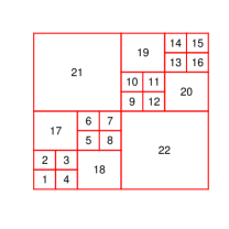
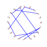
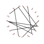
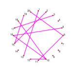
(a)	(b)	(c)	(d)

Figure 1: (a) The 22 subregions defined on $[0,1]^{2}$. The horizontal axis corresponds to the first dimension denoted as $X_{1}$ while the vertical axis corresponds to the second dimension denoted as $X_{2}$. The bottom left point corresponds to $[0,0]$ and the upper right point corresponds to $[1,1]$. (b) The true graph for subregion 4. (c) The true graph for subregion 17. (d) The true graph for subregion 22.

To each data point $x_{i}$ in the $t$-th subregion we associate a 20-dimensional response vector $y_{i}$ generated from a multivariate Gaussian distribution $N_{20}\left(0,\bigl{(}\Omega^{t}\right)^{-1}\bigr{)}$. We also create an equally-sized held-out dataset in the same manner based on $\{\Omega^{t}\}_{t=1}^{22}$.

We apply Algorithm 1 to this synthetic dataset. The estimated dyadic tree structure and its induced partitions are presented in Figure 2. Estimated graphs for some nodes are also illustrated. Note that the label for each subregion in subplot (c) is the leaf node ID of the tree in subplot (a). We conduct 100 Monte-Carlo simulations and find that in 82 out of 100 runs our algorithm perfectly recovers the ground truth partition of the $X_{1}$-$X_{2}$ plane, and never wrongly splits on any of the irrelevant dimensions, ranging from $X_{3}$ to $X_{10}$. Moreover, the estimated graphs have interesting patterns. Even though the graphs within each subregion are sparse, the estimated graph obtained by pooling all the data together is highly dense. As the algorithm progresses, the estimated graphs become more sparse. However, for the immediate parent nodes of the true subregions, the graphs become denser again.

Out of the 82 simulations where we correctly identify the tree structure, we list the graph estimation performance for subregions 1, 4, 17, 18, 21, 22 in terms of precision, recall, and $F_{1}$-score. Let $\widehat{E}$ be the estimated edge set while $E$ be the true edge set. These criteria are defined as:

$$\text{precision}=\frac{|\widehat{E}\cap E|}{|\widehat{E}|},~{}~{}\text{recall}=\frac{|\widehat{E}\cap E|}{|E|},~{}~{}F_{1}\text{-score}=2\cdot\frac{\text{precision}\cdot\text{recall}}{\text{precision}+\text{recall}}.$$ (5.1)

We see that for a larger subregion, it is easier to obtain better recovery performance, while good recovery for a very small region is more challenging. Of course, in the smaller regions there is less data. In Figure 1(a), there are only $10000/64\thickapprox 156$ data points that appear in subregion 1 (the smallest one). In contrast, approximately $10000/16=625$ data points fall inside subregion 18, so that the graph corresponding to this region can be better estimated.

We also plot the held-out risk in the subplot (c). As can be seen, the first few splits lead to the most significant decrease in the held-out risk.

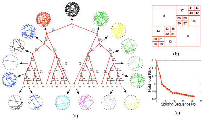
Figure 2: (a) The estimated dyadic tree structure; (b) the induced partition on $[0,1]^{2}$ and the number labeled on each subregion corresponds to each leaf node ID of the tree in (a); (c) the held-out negative log-likelihood risk for each split. The order of the splits corresponds the ID of the tree node (from small to large)

Further simulations where the ground truth covariance matrix is a continuous function of $x$ are presented in the appendix.

Table 1: Graph estimation performance over different subregions

Mean values over 100 runs (Standard deviation)
$\displaystyle\mathbf{subregion}$	region 1	region 4	region 17	region 18	region 21	region 22
$\displaystyle\mathrm{Precision}$	$0.8327\ (0.15)$	$0.8429\ (0.15)$	$0.9821\ (0.05)$	$0.9853\ (0.04)$	$0.9906\ (0.04)$	$0.9899\ (0.05)$
$\displaystyle\mathrm{Recall}$	$0.7890\ (0.16)$	$0.7990\ (0.18)$	$1.0000\ (0.00)$	$1.0000\ (0.00)$	$1.0000\ (0.00)$	$1.0000\ (0.00)$
$\displaystyle F_{1}-\mathrm{score}$	$0.7880\ (0.11)$	$0.7923\ (0.12)$	$0.9904\ (0.03)$	$0.9921\ (0.02)$	$0.9949\ (0.02)$	$0.9913\ (0.02)$

5.2 Climate Data Analysis

In this section, we use graph-valued regression to analyze a meteorology dataset (Lozano et al., 2009) that contains monthly data of 18 different meteorological factors from 1990 to 2002. We use the data from 1990 to 1995 as the training data and the data from 1996 to 2002 as the held-out validation data. The observations span 125 locations in the US on an equally spaced grid between latitude 30.475 and 47.975 and longitude -119.75 to -82.25. The 18 meteorological factors measured for each month include levels of CO₂, CH₄, H₂, CO, average temperature (TMP) and diurnal temperature range (DTR), minimum temperate (TMN), maximum temperature (TMX), precipitation (PRE), vapor (VAP), cloud cover (CLD), wet days (WET), frost days (FRS), global solar radiation (GLO), direct solar radiation (DIR), extraterrestrial radiation (ETR), extraterrestrial normal radiation (ETRN) and UV aerosol index (UV). For further detail, see Lozano et al. (2009).

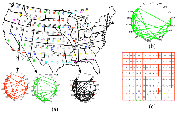
Figure 3: Analysis of the climate data. (a) Estimated partitions for 125 locations projected to the US map, with the estimated graphs for subregions 2, 3, and 65; (b) estimated graph with data pooled from all 125 locations; (c) the re-scaled partition pattern induced by the dyadic tree structure.

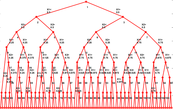
Figure 4: The estimated dyadic tree structure on the climate data.

As a baseline, we estimate a sparse graph on the data from all 125 locations, using the glasso algorithm; the estimated graph is shown in Figure 3 (b). It is seen that there is no edge connecting to any of the greenhouse gas factors CO₂, CH₄, H₂ or CO. This apparently contradicts basic domain knowledge that these four factors should correlate with the solar radiation factors (including GLO, DIR, ETR, ETRN, and UV), according to the 2007 report of the Intergovermental Panel on Climate Change IPCC (2007).The reason for the missing edges in the pooled data may be that positive correlations at one location are canceled by negative correlations at other locations.

Treating the longitude and latitude of each site as two-dimensional covariate $X$, and the meteorology data of the $p=18$ factors as the response $Y$, we estimate a dyadic tree structure using the greedy algorithm. The result is a partition with 87 subregions, shown in Figure 3, with the corresponding dyadic partition tree is shown in Figure 4. The graphs for subregion 2 (corresponding to the strip of land from Los Angeles, California to Phoenix, Arizona) and subregion 3 (Bakersfield, California to Flagstaff, Arizona) are shown in subplot (a) of Figure 3. The graphs for these two adjacent subregions are quite similar, suggesting spatial smoothness of the learned graphs. Moreover, for both graphs, CO is connected to solar radiation factors in either a direct or indirect way, and H₂ is connected to UV, which is accordance with Chapter 7 of the IPCC report IPCC (2007). In contrast, for subregion 65, which corresponds to the border of South Dakota and Nebraska; here the graph is quite different. In general, it is found that the graphs corresponding to the locations along the coasts are sparser than those corresponding to more central locations in the mainland.

Such observations, which require validation and interpretation by domain experts, are examples of the capability of graph-valued regression to provide a useful tool for high dimensional data analysis.

6 Conclusions

In this paper, we present Go-CART, a partition-based estimator of the family of undirected graphs associated with a high dimensional conditional distribution. Dyadic partitioning estimators, either using penalized empirical risk minimization or data splitting, are attractive due to their simplicity and theoretical guarantees. We derive finite sample oracle inequalities on excess risk, together with a tree partition consistency result. Our theory allows the scale of the graphs to increase with the sample size, which is relevant since the methods are targeted at high dimensional data analysis applications. Greedy partitioning estimators are proposed that are computationally attractive, combining classical greedy algorithms for decision trees with recent advances in $\ell_{1}$-regularization techniques for graph selection. The practical potential of Go-CART is indicated by experiments on a meteorology dataset. A theoretical analysis of greedy Go-CART is one of several interesting directions for future work.

Appendix A Proofs of Technical Results

A.1 Proof of Theorem 4.1

For any $T\in\mathcal{T}_{N}$, we denote

$$S_{j,n}=\frac{1}{n}\sum_{i=1}^{n}(y_{i}-\mu_{\mathcal{X}_{j}})(y_{i}-\mu_{\mathcal{X}_{j}})^{T}\cdot I(x_{i}\in\mathcal{X}_{j})$$ (A.1)

$$\bar{S}_{j}=\mathbb{E}(Y-\mu_{\mathcal{X}_{j}})(Y-\mu_{\mathcal{X}_{j}})^{T}\cdot I(X\in\mathcal{X}_{j}).$$ (A.2)

We then have

$$\left|R(T,\mu_{T},\Omega_{T})-\widehat{R}(T,\mu_{T},\Omega_{T})\right|$$ (A.3)

$$\leq \biggl{|}\sum_{j=1}^{m}\mathrm{tr}\left[\Omega_{\mathcal{X}_{j}}\left(S_{j,n}-\bar{S}_{j}\right)\right]\biggr{|}+\biggl{|}\sum_{j=1}^{m}\log|\Omega_{\mathcal{X}_{j}}|\cdot\Bigl{[}\frac{1}{n}\sum_{i=1}^{n}I(x_{i}\in\mathcal{X}_{j})-\mathbb{E}I(X\in\mathcal{X}_{j})\Bigr{]}\biggr{|}$$

$$\leq \underbrace{\sum_{j=1}^{m}\|\Omega_{\mathcal{X}_{j}}\|_{1}\cdot\left\|S_{j,n}-\bar{S}_{j}\right\|_{\infty}}_{A_{1}}+\underbrace{\sum_{j=1}^{m}\Bigl{|}\log|\Omega_{\mathcal{X}_{j}}|\Bigr{|}\cdot\biggl{|}\frac{1}{n}\sum_{i=1}^{n}I(x_{i}\in\mathcal{X}_{j})-\mathbb{E}I(X\in\mathcal{X}_{j})\biggr{|}}_{A_{2}}.$$ (A.4)

We now analyze the terms $A_{1}$ and $A_{2}$ separately.

For $A_{2}$, using the Hoeffding’s inequality, for $\epsilon>0$, we get

$$\mathbb{P}\left(\biggl{|}\frac{1}{n}\sum_{i=1}^{n}I(x_{i}\in\mathcal{X}_{j})-\mathbb{E}I(X\in\mathcal{X}_{j})\biggr{|}>\epsilon\right)\leq 2\exp\left(-2n\epsilon^{2}\right),$$ (A.5)

which implies that,

$$\mathbb{P}\Biggl{(}\sup_{T\in\mathcal{T}_{N}}\biggl{|}\frac{1}{n}\sum_{i=1}^{n}I(x_{i}\in\mathcal{X}_{j})-\mathbb{E}I(X\in\mathcal{X}_{j})\biggr{|}/\epsilon_{T}>1\Biggr{)}\leq 2\sum_{T\in\mathcal{T}_{N}}\exp\left(-2n\epsilon^{2}_{T}\right),$$ (A.6)

where $\epsilon_{T}$ means $\epsilon$ is a function of $T$. For any $\delta\in(0,1)$, we have, with probability at least $1-\delta/4$,

$$\forall T\in\mathcal{T}_{N},~{}\biggl{|}\frac{1}{n}\sum_{i=1}^{n}I(x_{i}\in\mathcal{X}_{j})-\mathbb{E}I(X\in\mathcal{X}_{j})\biggr{|}\leq\sqrt{\frac{[[T]]\log 2+\log(8/\delta)}{2n}}$$ (A.7)

where $[[T]]>0$ is the prefix code of $T$ given in (3.3).

From Assumption 4.1, since $\Omega_{\mathcal{X}_{j}}\in\Lambda_{j}$, we have that

$$\max_{1\leq j\leq m_{T}}\log\left|\Omega_{\mathcal{X}_{j}}\right|\leq L_{n}$$ (A.8)

Therefore, with probability at least $1-\delta/4$,

$$A_{2}\leq L_{n}m_{T}\sqrt{\frac{[[T]]\log 2+\log(8/\delta)}{2n}}.$$ (A.9)

Next, we analyze the term $A_{1}$. Since

$$\max_{1\leq j\leq m_{T}}\|\Omega_{\mathcal{X}_{j}}\|_{1}\leq L_{n}.$$ (A.10)

we only need to bound the term $\left\|S_{j,n}-\bar{S}_{j}\right\|_{\infty}$. By Assumption 4.2 and the union bound, we have, for any $\epsilon>0$,

$$\mathbb{P}\left(\left\|S_{j,n}-\bar{S}_{j}\right\|_{\infty}>\epsilon\right)$$ (A.14)

$$\leq \mathbb{P}\biggl{(}\Bigl{\|}\frac{1}{n}\sum_{i=1}^{n}y_{i}y^{T}_{i}I(x_{i}\in\mathcal{X}_{j})-\mathbb{E}\bigl{[}YY^{T}I(X\in\mathcal{X}_{j})\bigr{]}\Bigr{\|}_{\infty}>\frac{\epsilon}{4}\biggr{)}$$

$$+\mathbb{P}\biggl{(}\Bigl{\|}\frac{1}{n}\sum_{i=1}^{n}y_{i}\mu^{T}_{\mathcal{X}_{j}}I(x_{i}\in\mathcal{X}_{j})-\mathbb{E}\bigl{[}Y\mu^{T}_{\mathcal{X}_{j}}I(X\in\mathcal{X}_{j})\bigr{]}\Bigr{\|}_{\infty}>\frac{\epsilon}{4}\biggr{)}$$

$$+\mathbb{P}\biggl{(}\Bigl{\|}\frac{1}{n}\sum_{i=1}^{n}\mu_{\mathcal{X}_{j}}y^{T}_{i}I(x_{i}\in\mathcal{X}_{j})-\mathbb{E}\bigl{[}\mu_{\mathcal{X}_{j}}Y^{T}I(X\in\mathcal{X}_{j})\bigr{]}\Bigr{\|}_{\infty}>\frac{\epsilon}{4}\biggr{)}$$

$$+\mathbb{P}\biggl{(}\Bigl{\|}\frac{1}{n}\sum_{i=1}^{n}\mu_{\mathcal{X}_{j}}\mu^{T}_{\mathcal{X}_{j}}I(x_{i}\in\mathcal{X}_{j})-\mathbb{E}\bigl{[}\mu_{\mathcal{X}_{j}}\mu^{T}_{\mathcal{X}_{j}}I(X\in\mathcal{X}_{j})\bigr{]}\Bigr{\|}_{\infty}>\frac{\epsilon}{4}\biggr{)}.$$

Using the fact that $\|\mu\|_{\infty}\leq B$ and the Assumption 4.2, we can apply Bernstein’s exponential inequality on (A.14), (A.14), and (A.14). Also, since the indicator function is bounded, we can apply Hoeffding’s inequality on (A.14). In this way we obtain

$$\mathbb{P}\left(\left\|S_{j,n}-\bar{S}_{j}\right\|_{\infty}>\epsilon\right)$$

$$\leq 2p^{2}\exp\left(-\frac{1}{32}\biggl{(}\frac{n\epsilon^{2}}{v_{2}+M_{2}\epsilon}\biggr{)}\right)+4p^{2}\exp\left(-\frac{1}{32B^{2}}\biggl{(}\frac{n\epsilon^{2}}{v_{1}+M_{1}\epsilon}\biggr{)}\right)+2p^{2}\exp\left(-\frac{2n\epsilon^{2}}{B^{4}}\right).$$

Therefore, for any $\delta\in(0,1)$, we have, for any $\epsilon\rightarrow 0$ as $n$ goes to infinity, with probability at least $1-\delta/4$

$$\forall T\in\mathcal{T}_{N},~{}\left\|S_{j,n}-\bar{S}_{j}\right\|_{\infty} \leq (8\sqrt{v_{2}})\cdot\sqrt{\frac{[[T]]\log 2+2\log p+\log(24/\delta)}{n}}$$ (A.16)

$$+ (8B\sqrt{v_{1}})\cdot\sqrt{\frac{[[T]]\log 2+2\log p+\log(48/\delta)}{n}}$$ (A.17)

$$+ B^{2}\cdot\sqrt{\frac{[[T]]\log 2+2\log p+\log(24/\delta)}{2n}}$$ (A.18)

Combined with (A.10), we get that

$$A_{1}\leq C_{1}L_{n}m_{T}\sqrt{\frac{[[T]]\log 2+2\log p+\log(48/\delta)}{n}}.$$ (A.19)

where $C_{1}=8\sqrt{v_{2}}+8B\sqrt{v_{1}}+B^{2}$.

Since the above analysis holds uniformly over $\mathcal{T}_{N}$, when choosing

$$\mathrm{pen}(T)=(C_{1}+1)L_{n}m_{T}\sqrt{\frac{[[T]]\log 2+2\log p+\log(48/\delta)}{n}},$$ (A.20)

we then get, with probability at least $1-\delta/2$,

$$\sup_{T\in\mathcal{T}_{N},\mu_{j}\in M_{j},\Omega_{j}\in\Lambda_{j}}\left|R(T,\mu_{T},\Omega_{T})-\widehat{R}(T,\mu_{T},\Omega_{T})\right|\leq\mathrm{pen}(T)$$ (A.21)

for large enough $n$.

Given a DPT $T$, we define

$$\mu^{o}_{T},\Omega^{o}_{T}=\mathop{\text{\rm arg\,min}}_{\mu_{T}\in M_{j},\Omega_{T}\in\Lambda_{j}}R(T,\mu_{T},\Omega_{T}).$$ (A.22)

From the uniform deviation inequality in (A.21), we have, for large enough $n$: for any $\delta\in(0,1)$, with probability at least $1-\delta$,

$$R(\widehat{T},\widehat{\mu}_{\widehat{T}},\widehat{\Omega}_{\widehat{T}}) \leq \widehat{R}(\widehat{T},\widehat{\mu}_{\widehat{T}},\widehat{\Omega}_{\widehat{T}})+\mathrm{pen}(\widehat{T})$$ (A.23)

$$= \inf_{T\in\mathcal{T}_{N},\mu_{\mathcal{X}_{j}}\in M_{j},\Omega_{\mathcal{X}_{j}}\in\Lambda_{j}}\biggl{\{}\widehat{R}(T,\mu_{T},\Omega_{T})+\mathrm{pen}(T)\biggr{\}}$$ (A.24)

$$\leq \inf_{T\in\mathcal{T}_{N}}\left\{\widehat{R}(T,\mu^{0}_{T},\Omega^{0}_{T})+\mathrm{pen}(T)\right\}$$ (A.25)

$$\leq \inf_{T\in\mathcal{T}_{N}}\left\{{R}(T,\mu^{0}_{T},\Omega^{0}_{T})+2\mathrm{pen}(T)\right\}$$ (A.26)

$$= \inf_{T\in\mathcal{T}_{N}}\left\{\inf_{\mu_{\mathcal{X}_{j}}\in M_{j},\Omega_{\mathcal{X}_{j}}\in\Lambda_{j}}(R(T,\mu_{T},\Omega_{T})+2\mathrm{pen}(T)\right\}.$$ (A.27)

The desired result of the theorem follows by subtracting $R^{*}$ from both sides.

A.2 Proof of Theorem 4.2

From (A.21) we have, for large enough $n$, on the dataset $\mathcal{D}_{1}$, with probability at least $1-{\delta}/{4}$

$$\sup_{T\in\mathcal{T}_{N},\mu_{j}\in M_{j},\Omega_{j}\in\Lambda_{j}}\left|R(T,\mu_{T},\Omega_{T})-\widehat{R}(T,\mu_{T},\Omega_{T})\right|\leq\phi_{n}(T).$$ (A.28)

Following the same line of analysis, we can also get that on the validation dataset $\mathcal{D}_{2}$, with probability at least $1-\delta/4$,

$$\sup_{T\in\mathcal{T}_{N}}\left|R(T,\widehat{\mu}_{T},\widehat{\Omega}_{T})-\widehat{R}_{\rm out}(T,\widehat{\mu}_{T},\widehat{\Omega}_{T})\right|\leq\phi_{n}(T)$$ (A.29)

for large enough $n$. Here $\widehat{\mu}_{T},\widehat{\Omega}_{T}$ are as defined in (3.6).

Given a DPT $T$, we define

$$\mu^{o}_{T},\Omega^{o}_{T}=\mathop{\text{\rm arg\,min}}_{\mu_{T}\in M_{j},\Omega_{T}\in\Lambda_{j}}R(T,\mu_{T},\Omega_{T}).$$ (A.30)

Using the fact that

$$\widehat{T}=\displaystyle{\rm argmin}_{T\in\mathcal{T}_{N}}\widehat{R}_{\rm out}(T,\widehat{\mu}_{T},\widehat{\Omega}_{T}),$$ (A.31)

we have, for large enough $n$ and any $\delta\in(0,1)$, with probability at least $1-\delta$,

$$R(\widehat{T},\widehat{\mu}_{\widehat{T}},\widehat{\Omega}_{\widehat{T}}) \leq \widehat{R}_{\rm out}(\widehat{T},\widehat{\mu}_{\widehat{T}},\widehat{\Omega}_{\widehat{T}})+\phi_{n}(\widehat{T})$$ (A.32)

$$= \inf_{T\in\mathcal{T}_{N}}\widehat{R}_{\rm out}(T,\widehat{\mu}_{T},\widehat{\Omega}_{T})+\phi_{n}(\widehat{T})$$ (A.33)

$$\leq \inf_{T\in\mathcal{T}_{N}}\left\{R(T,\widehat{\mu}_{T},\widehat{\Omega}_{T})+\phi_{n}(T)\right\}+\phi_{n}(\widehat{T})$$ (A.34)

$$\leq \inf_{T\in\mathcal{T}_{N}}\left\{\widehat{R}(T,\widehat{\mu}_{T},\widehat{\Omega}_{T})+\phi_{n}(T)+\phi_{n}(T)\right\}+\phi_{n}(\widehat{T})$$ (A.35)

$$\leq \inf_{T\in\mathcal{T}_{N}}\left\{\widehat{R}(T,\mu^{0}_{T},\Omega^{0}_{T})+\phi_{n}(T)+\phi_{n}(T)\right\}+\phi_{n}(\widehat{T})$$

$$\leq \inf_{T\in\mathcal{T}_{N}}\left\{3\phi_{n}(T)+\inf_{\mu_{\mathcal{X}_{j}}\in M_{j},\Omega_{\mathcal{X}_{j}}\in\Lambda_{j}}R(T,\mu_{T},\Omega_{T})\right\}+\phi_{n}(\widehat{T}).$$

The result follows by subtracting $R^{*}$ from both sides.

A.3 Proof of Theorem 4.3

For any $T\in\mathcal{T}_{N}$, $\Pi(T^{*})\nsubseteq\Pi(T)$, there must exist a subregion $\mathcal{X}^{\prime}\in\Pi(T)$ such that no $\mathcal{A}\in\Pi(T^{*})$ satisfies $\mathcal{X}^{\prime}\subset\mathcal{A}$. We can thus find a minimal class of disjoint subregions $\{\mathcal{X}^{0}_{1},\ldots,\mathcal{X}^{0}_{k^{\prime}}\}\in\Pi(T^{*})$, such that

$$\mathcal{X}^{\prime}\subset\cup_{i=1}^{k^{\prime}}\mathcal{X}^{0}_{i},$$ (A.37)

where $k^{\prime}\geq 2$. We define $\mathcal{X}^{*}_{i}=X^{0}_{i}\cap\mathcal{X}^{\prime}$ for $i=1,\ldots,k^{\prime}$. Then we have

$$\mathcal{X}^{\prime}=\cup_{i=1}^{k^{\prime}}\mathcal{X}^{*}_{i}.$$ (A.38)

Let $\{\mu^{*}_{\mathcal{X}^{*}_{j}},\Omega^{*}_{\mathcal{X}^{*}_{j}}\}_{j=1}^{k^{\prime}}$ be the true parameters on $\mathcal{X}^{0}_{1},\ldots,\mathcal{X}^{0}_{k^{\prime}}$. We denote by $R(\mathcal{X}^{\prime},\mu^{*}_{T^{*}},\Omega^{*}_{T^{*}})$ the risk of $\mu^{*}_{T^{*}}$ and $\Omega^{*}_{T^{*}}$ on the subregion $\mathcal{X}^{\prime}$, so that

$$R(\mathcal{X}^{\prime},\mu^{*}_{T^{*}},\Omega^{*}_{T^{*}}) = \sum_{j=1}^{k^{\prime}}\mathbb{E}\biggl{[}\left(\mathrm{tr}\left[\Omega^{*}_{\mathcal{X}^{*}_{j}}\bigl{(}(Y-\mu^{*}_{\mathcal{X}^{*}_{j}})(Y-\mu^{*}_{\mathcal{X}^{*}_{j}})^{T}\bigr{)}\right]-\log|\Omega^{*}_{\mathcal{X}^{*}_{j}}|\right)\cdot I(X\in\mathcal{X}^{*}_{j})\biggr{]}$$ (A.39)

$$= p\mathbb{P}\left(X\in\mathcal{X}^{\prime}\right)-\sum_{j=1}^{k^{\prime}}\mathbb{P}\left(X\in\mathcal{X}^{*}_{j}\right)\log|\Omega^{*}_{\mathcal{X}^{*}_{j}}|.$$

Since the DPT $T$ does not further partition $\mathcal{X}^{\prime}$, we have, for any $\mu_{T},\Omega_{T}\in\mathcal{M}_{T}$

$$R(\mathcal{X}^{\prime},\mu_{T},\Omega_{T})$$

$$= \sum_{j=1}^{k^{\prime}}\mathbb{E}\biggl{[}\Bigl{(}\mathrm{tr}\left[\Omega_{T}\left((Y-\mu_{T})(Y-\mu_{T})^{T}\right)\right]-\log|\Omega_{T}|\Bigr{)}\cdot I(X\in\mathcal{X}^{*}_{j})\biggr{]}$$

$$= \sum_{j=1}^{k^{\prime}}\mathbb{E}\biggl{[}\Bigl{(}\mathrm{tr}\left[\Omega_{T}\left((Y-\mu_{T})(Y-\mu_{T})^{T}\right)\right]\Bigr{)}\cdot I(X\in\mathcal{X}^{*}_{j})\biggr{]}-\mathbb{P}(X\in\mathcal{X}^{\prime})\log|\Omega_{T}|.$$

Using the decomposition

$$(Y-\mu_{T})(Y-\mu_{T})^{T}=(Y-\mu^{*}_{\mathcal{X}^{*}_{j}})(Y-\mu^{*}_{\mathcal{X}^{*}_{j}})^{T}+(Y-\mu^{*}_{\mathcal{X}^{*}_{j}})(\mu^{*}_{\mathcal{X}^{*}_{j}}-\mu_{T})^{T}$$ (A.40)

$$~{}~{}~{}~{}~{}~{}~{}~{}~{}~{}~{}~{}~{}+(\mu^{*}_{\mathcal{X}^{*}_{j}}-\mu_{T})(Y-\mu^{*}_{\mathcal{X}^{*}_{j}})^{T}+(\mu^{*}_{\mathcal{X}^{*}_{j}}-\mu_{T})(\mu^{*}_{\mathcal{X}^{*}_{j}}-\mu_{T})^{T}$$

we obtain

$$\sum_{j=1}^{k^{\prime}}\mathbb{E}\biggl{[}\Bigl{(}\mathrm{tr}\left[\Omega_{T}\left((Y-\mu_{T})(Y-\mu_{T})^{T}\right)\right]\Bigr{)}\cdot I(X\in\mathcal{X}^{*}_{j})\biggr{]}$$ (A.41)

$$= \sum_{j=1}^{k^{\prime}}\mathbb{P}\left(X\in\mathcal{X}^{*}_{j}\right)\left[\mathrm{tr}(\Omega_{T}(\Omega^{*}_{j})^{-1})+\mathrm{tr}(\Omega_{T}(\mu^{*}_{\mathcal{X}^{*}_{j}}-\mu_{T})(\mu^{*}_{\mathcal{X}^{*}_{j}}-\mu_{T})^{T})\right].$$

Using the bound

$$R(\mathcal{X}^{\prime},\mu_{T},\Omega_{T})\geq\max\{R(\mathcal{X}^{\prime},\mu^{*}_{T^{*}},\Omega_{T}),R(\mathcal{X}^{\prime},\mu_{T},\Omega^{*}_{T^{*}})\},$$ (A.42)

we proceed by cases.

Case 1: The $\mu$’s are different. We know that

$$\inf_{\mu_{T},\Omega_{T}\in\mathcal{M}_{T}}R(\mathcal{X}^{\prime},\mu_{T},\Omega_{T})-R(\mathcal{X}^{\prime},\mu^{*}_{T^{*}},\Omega^{*}_{T^{*}})$$

$$\geq \inf_{\mu_{T}}R(\mathcal{X}^{\prime},\mu_{T},\Omega^{*}_{T^{*}})-R(\mathcal{X}^{\prime},\mu^{*}_{T^{*}},\Omega^{*}_{T^{*}})$$

$$= \inf_{\mu_{T}}\sum_{j=1}^{k^{\prime}}\mathbb{P}\left(X\in\mathcal{X}^{*}_{j}\right)(\mu^{*}_{\mathcal{X}^{*}_{j}}-\mu_{T})^{T}\Omega^{*}_{\mathcal{X}^{*}_{j}}(\mu^{*}_{\mathcal{X}^{*}_{j}}-\mu_{T})$$

$$\geq c_{1}c_{2}\inf_{\mu_{T}}\sum_{j=1}^{k^{\prime}}\|\mu^{*}_{\mathcal{X}^{*}_{j}}-\mu_{T}\|^{2}_{2}$$

where the last inequality follows from that fact that $\rho_{\rm\min}(\Omega^{*}_{\mathcal{X}^{*}_{j}})\geq c_{1},\mathbb{P}\left(X\in\mathcal{X}^{*}_{j}\right)\geq c_{2}$. It’s easy to see that a lower bound of the last term is achieved at $\bar{\mu}_{T}$,

$$\bar{\mu}_{T}=\frac{1}{k^{\prime}}\sum_{j=1}^{k^{\prime}}\mu^{*}_{\mathcal{X}^{*}_{j}}.$$ (A.44)

Furthermore, for any two DPTs $T$ and $T^{\prime}$, if $\Pi(T)\subset\Pi(T^{\prime})$ it’s clear that

$$\inf_{\mu_{T},\Omega_{T}\in\mathcal{M}_{T}}R(T,\mu_{T},\Omega_{T})\geq\inf_{\mu_{T^{\prime}},\Omega_{T^{\prime}}\in\mathcal{M}_{T^{\prime}}}R(T^{\prime},\mu_{T^{\prime}},\Omega_{T^{\prime}}).$$ (A.45)

Therefore, in the sequel, without loss of generality we only need to consider the case $k^{\prime}=2$.

The result in this case then follows from the fact that

$$\sum_{j=1}^{2}\|\mu^{*}_{\mathcal{X}^{*}_{j}}-\bar{\mu}_{T}\|^{2}_{2}=\frac{1}{2}\|\mu_{\mathcal{X}^{*}_{1}}-\mu_{\mathcal{X}^{*}_{2}}\|^{2}_{2}\geq\frac{c_{3}}{2}.$$ (A.46)

Case 2: The $\Omega$’s are different. In this case, we have

$$\inf_{\mu_{T},\Omega_{T}\in\mathcal{M}_{T}}R(\mathcal{X}^{\prime},\mu_{T},\Omega_{T})-R(\mathcal{X}^{\prime},\mu^{*}_{T^{*}},\Omega^{*}_{T^{*}})\geq\inf_{\Omega_{T}}R(\mathcal{X}^{\prime},\mu^{*}_{T^{*}},\Omega_{T})-R(\mathcal{X}^{\prime},\mu^{*}_{T^{*}},\Omega^{*}_{T^{*}})$$ (A.47)

$$= \inf_{\Omega_{T}}\sum_{j=1}^{k^{\prime}}\mathbb{P}\left(X\in\mathcal{X}^{*}_{j}\right)\left(\mathrm{tr}\left[\Omega^{-1}_{\mathcal{X}^{*}_{j}}(\Omega_{T}-\Omega^{*}_{\mathcal{X}^{*}_{j}})\right]-\left(\log|\Omega_{T}|-\log|\Omega^{*}_{\mathcal{X}^{*}_{j}}|\right)\right)$$

$$\geq c_{2}\inf_{\Omega_{T}}\sum_{j=1}^{k^{\prime}}\left(\mathrm{tr}\left[\Omega^{-1}_{\mathcal{X}^{*}_{j}}(\Omega_{T}-\Omega^{*}_{\mathcal{X}^{*}_{j}})\right]-\left(\log|\Omega_{T}|-\log|\Omega^{*}_{\mathcal{X}^{*}_{j}}|\right)\right)$$ (A.48)

$$\geq c_{2}\inf_{\Sigma_{T}}\sum_{j=1}^{k^{\prime}}\left(\mathrm{tr}\left[\Sigma^{*}_{\mathcal{X}^{*}_{j}}(\Sigma^{-1}_{T}-\Omega^{*}_{\mathcal{X}^{*}_{j}})\right]+\log\frac{|\Sigma_{T}|}{|\Sigma^{*}_{\mathcal{X}^{*}_{j}}|}\right)$$ (A.49)

$$= c_{2}\inf_{\Sigma_{T}}\sum_{j=1}^{k^{\prime}}\left(\mathrm{tr}\left(\Sigma^{*}_{\mathcal{X}^{*}_{j}}\Sigma^{-1}_{T}\right)+\log\frac{|\Sigma_{T}|}{|\Sigma^{*}_{\mathcal{X}^{*}_{j}}|}-p\right)$$ (A.50)

where $\Sigma_{T}=\Omega^{-1}_{T}$.

As before, we only need to consider the case $k^{\prime}=2$. A lower bound of the last term is achieved at

$$\bar{\Sigma}_{T}=\frac{\Sigma_{\mathcal{X}^{*}_{1}}+\Sigma_{\mathcal{X}^{*}_{2}}}{2}.$$ (A.51)

Plugging in $\bar{\Sigma}_{T}$, we get

$$\inf_{\Sigma_{T}}\sum_{j=1}^{2}\left(\mathrm{tr}\left(\Sigma^{*}_{\mathcal{X}^{*}_{j}}\Sigma^{-1}_{T}\right)+\log\frac{|\Sigma_{T}|}{|\Sigma^{*}_{\mathcal{X}^{*}_{j}}|}-p\right)\geq\sum_{j=1}^{2}\left(\mathrm{tr}\left(\Sigma^{*}_{\mathcal{X}^{*}_{j}}\bar{\Sigma}^{-1}_{T}\right)+\log\frac{|\bar{\Sigma}_{T}|}{|\Sigma^{*}_{\mathcal{X}^{*}_{j}}|}-p\right)$$ (A.52)

$$= \mathrm{tr}\left((2\bar{\Sigma}_{T}-\Sigma_{\mathcal{X}^{*}_{2}})\bar{\Sigma}^{-1}_{T}\right)+\log\frac{|\bar{\Sigma}_{T}|}{|\Sigma_{\mathcal{X}^{*}_{1}}|}-p+\mathrm{tr}\left(\Sigma_{\mathcal{X}^{*}_{2}}\bar{\Sigma}^{-1}_{T}\right)+\log\frac{|\bar{\Sigma}_{T}|}{|\Sigma_{\mathcal{X}^{*}_{2}}|}-p$$

$$= \log\frac{|\bar{\Sigma}_{T}|}{|\Sigma_{\mathcal{X}^{*}_{1}}|}+\log\frac{|\bar{\Sigma}_{T}|}{|\Sigma_{\mathcal{X}^{*}_{2}}|}$$ (A.53)

$$= 2\log\left|\frac{\Sigma_{\mathcal{X}^{*}_{1}}+\Sigma_{\mathcal{X}^{*}_{2}}}{2}\right|-\log|\Sigma_{\mathcal{X}^{*}_{1}}|-\log|\Sigma_{\mathcal{X}^{*}_{2}}|$$ (A.54)

$$\geq c_{4}$$ (A.55)

where the last inequality follows from the given assumption.

Therefore, we have

$$\inf_{\mu_{T},\Omega_{T}\in\mathcal{M}_{T}}R(\mathcal{X}^{\prime},\mu_{T},\Omega_{T})-R(\mathcal{X}^{\prime},\mu^{*}_{T^{*}},\Omega^{*}_{T^{*}})\geq c_{2}c_{4}.$$ (A.56)

The theorem is obtained by combining the two cases.

Appendix B Further Simulations

To further demonstrate the performance of the method, this section presents simulations where the true conditional covariance matrix is continuous in $X$. We compare the graphs estimated by our method to the single graph obtained by applying the glasso directly to the entire dataset.

In this subsection, we consider the case where $X$ lies on a one dimensional chain. More precisely, we generate $n$ equally spaced points $x_{1},\ldots,x_{n}\in\mathbb{R}$ with $n=10,000$ on $[0,1]$. We generate an Erdös-Rényi random graph $G^{1}=(V^{1},E^{1})$ with $p=20$ vertices, $|E|=10$ edges, and maximum node degree four. Then, we simulate the output $y_{1},\ldots,y_{n}]\in\mathbb{R}^{p}$ as follows:

1. For $t=2$ to $T$, we construct the graph $G^{t}=(V^{t},E^{t})$ as follows: (a) with probability 0.05, remove one edge from $G^{t-1}$ and (b) with probability $0.05$, add one edge to the graph generated in (a). We make sure that the total number of edges is between 5 and 15, and that the maximum node degree four.

2. For each graph $G^{t}$, generate the inverse covariance matrix $\Omega^{t}$:

   $$\Omega^{t}(i,j)=\begin{cases}\ 1&\mathrm{if}~{}i=j,\\ 0.245&\mathrm{if}~{}(i,j)\in E^{t},\\ 0&\mathrm{otherwise,}\end{cases}$$

   where $0.245$ guarantees positive-definiteness of $\Omega^{t}$ under the degree constraint.

3. For each $t$, we sample $y_{t}$ from a multivariate Gaussian distribution with mean $\mu=(0,\ldots,0)\in\mathbb{R}^{p}$ and covariance matrix $\Sigma^{t}=(\Omega^{t})^{-1}$.

We generate an equal-sized held-out dataset in the same manner, using the same $\mu$ and $\Sigma^{t}$. Greedy Go-CART is used to estimate the dyadic tree structure and corresponding inverse covariance matrices; these are displayed in Figure 5.

B.1 Chain Structure

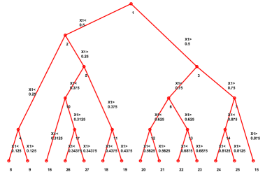
(a)	(b)

Figure 5: (a) Estimated tree structure; (b) corresponding partitions

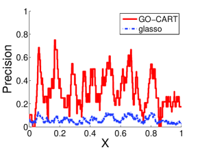
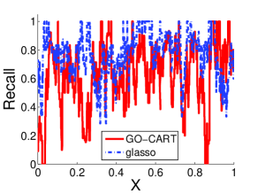
(a)	(b)
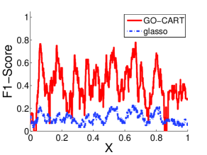
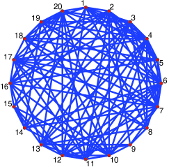
(c)	(d)

Figure 6: Comparison of our algorithm with glasso (a) Precision; (b) Recall; (c) $F_{1}$-score; (d) Estimated graph by applying glasso on the entire dataset

To examine the recovery quality of the underlying graph structure, we compare our estimated graphs to the graph estimated by directly applying the glasso to the entire dataset. Comparisons in terms of precision, recall and $F_{1}$-score are given in Figure 6 (a), (b) and (c) respectively. As we can see, the partition-based method achieves much higher precision and $F_{1}$-Score. As for recall, glasso is slightly better, due to the fact that the glasso graphs estimated on the entire data are very dense, as shown in 6 (d). The dense graphs lead to fewer false negatives (thus large recall) but many false positives (thus small precision).

B.2 Two-way Grid Structure

In this section, we apply Go-CART to a two dimensional design $X$. The underlying graph structures and $Y$ are generated in manner similar to that used in the previous section. In particular, we generate equally spaced $x_{1},\ldots,x_{n}\in\mathbb{R}^{2}$ with $n=10,000$ on the unit two-dimensional grid $[0,1]^{2}$. We generate an Erdös-Rényi random graph $G^{1,1}=(V^{1,1},E^{1,1})$ with $p=20$ vertices, $|E|=10$ edges, and maximum node degree four, then construct the graphs for each $x$ along diagonals. More precisely, for each pair of $i,j$, where $1\leq i\leq 100$ and $1\leq j\leq 100$, we randomly select either $G^{i-1,j}$ (if it exists) or $G^{i,j-1}$ (if it exists) with equal probability as the basis graph. Then, we construct the graph $G^{i,j}=(V^{i,j},E^{i,j})$ by removing one edge and adding one edge with probability $0.05$ based on the selected basis graph, taking care that the number of edges is between 5 and 15 and the maximum degree is still four. Given the underlying graphs, we generate the covariance matrix and output $Y$ in the same way as in the last section.

We apply the greedy algorithm to learn the dyadic tree structure and corresponding inverse covariance matrices, shown in Figure 7. We plot the $F_{1}$-score obtained by glasso on the entire data compared against the our method in Figure 8. It is seen that for most $x$, the partitioning method achieves significantly higher $F_{1}$-score than directly applying the glasso. Note that since the graphs near the middle part of the diagonal (the line connecting $[0,1]$ and $[1,0]$) have the greatest variability, the $F_{1}$-scores for both methods are low in this region.

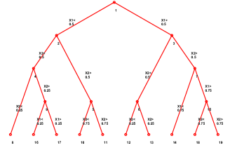
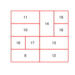
(a)	(b)

Figure 7: (a) Estimated tree structure; (b) estimated partitions where the labels correspond to the index of the leaf node in (a)

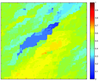
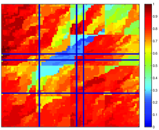
(a)	(b)

Figure 8: (a) Color map of $F_{1}$-score for glasso run on the entire dataset; (b) color map of $F_{1}$-score for Go-CART. Red indicates large values (approaching 1) and blue indicates small values (approaching 0), as shown in the color bar.

References

- Banerjee, Ghaoui and d’Aspremont (2008) {barticle}[author] \bauthor\bsnmBanerjee, \bfnmOnureena\binitsO., \bauthor\bsnmGhaoui, \bfnmLaurent El\binitsL. E. and \bauthor\bsnmd’Aspremont, \bfnmAlexandre\binitsA. (\byear2008). \btitleModel selection through sparse maximum likelihood estimation. \bjournalJournal of Machine Learning Research \bvolume9 \bpages485–516. \endbibitem
- Blanchard et al. (2007) {barticle}[author] \bauthor\bsnmBlanchard, \bfnmG.\binitsG., \bauthor\bsnmSchäfer, \bfnmC.\binitsC., \bauthor\bsnmRozenholc, \bfnmY.\binitsY. and \bauthor\bsnmMüller, \bfnmK.-R.\binitsK.-R. (\byear2007). \btitleOptimal dyadic decision trees. \bjournalMach. Learn. \bvolume66 \bpages209–241. \endbibitem
- Breiman et al. (1984) {bbook}[author] \bauthor\bsnmBreiman, \bfnmLeo\binitsL., \bauthor\bsnmFriedman, \bfnmJerome\binitsJ., \bauthor\bsnmStone, \bfnmCharles J.\binitsC. J. and \bauthor\bsnmOlshen, \bfnmR.A.\binitsR. (\byear1984). \btitleClassification and regression trees. \bpublisherWadsworth Publishing Co Inc. \endbibitem
- Edwards (1995) {bbook}[author] \bauthor\bsnmEdwards, \bfnmDavid\binitsD. (\byear1995). \btitleIntroduction to graphical modelling. \bpublisherSpringer-Verlag Inc. \endbibitem
- Friedman, Hastie and Tibshirani (2007) {barticle}[author] \bauthor\bsnmFriedman, \bfnmJerome H.\binitsJ. H., \bauthor\bsnmHastie, \bfnmTrevor\binitsT. and \bauthor\bsnmTibshirani, \bfnmRobert\binitsR. (\byear2007). \btitleSparse inverse covariance estimation with the graphical lasso. \bjournalBiostatistics \bvolume9 \bpages432–441. \endbibitem
- IPCC (2007) {barticle}[author] \bauthor\bsnmIPCC, (\byear2007). \btitleClimate Change 2007–The Physical Science Basis IPCC Fourth Assessment Report. \endbibitem
- Lauritzen (1996) {bbook}[author] \bauthor\bsnmLauritzen, \bfnmSteffen L.\binitsS. L. (\byear1996). \btitleGraphical Models. \bpublisherOxford University Press. \endbibitem
- Liu, Lafferty and Wasserman (2010) {bunpublished}[author] \bauthor\bsnmLiu, \bfnmHan\binitsH., \bauthor\bsnmLafferty, \bfnmJohn\binitsJ. and \bauthor\bsnmWasserman, \bfnmLarry\binitsL. (\byear2010). \btitleTree Density Estimation. \bnotearXiv:1001.1557v1 [stat.ML] 10 Jan 2010. \endbibitem
- Lozano et al. (2009) {binproceedings}[author] \bauthor\bsnmLozano, \bfnmAurelie C.\binitsA. C., \bauthor\bsnmLi, \bfnmHongfei\binitsH., \bauthor\bsnmNiculescu-Mizil, \bfnmAlexandru\binitsA., \bauthor\bsnmLiu, \bfnmYan\binitsY., \bauthor\bsnmPerlich, \bfnmClaudia\binitsC., \bauthor\bsnmHosking, \bfnmJonathan\binitsJ. and \bauthor\bsnmAbe, \bfnmNaoki\binitsN. (\byear2009). \btitleSpatial-temporal causal modeling for climate change attribution. In \bbooktitleACM SIGKDD. \endbibitem
- Ravikumar et al. (2009) {binproceedings}[author] \bauthor\bsnmRavikumar, \bfnmPradeep\binitsP., \bauthor\bsnmWainwright, \bfnmMartin\binitsM., \bauthor\bsnmRaskutti, \bfnmGarvesh\binitsG. and \bauthor\bsnmYu, \bfnmBin\binitsB. (\byear2009). \btitleModel Selection in Gaussian Graphical Models: High-Dimensional Consistency of -regularized MLE. In \bbooktitleAdvances in Neural Information Processing Systems 22. \bpublisherMIT Press, \baddressCambridge, MA. \endbibitem
- Rothman et al. (2008) {barticle}[author] \bauthor\bsnmRothman, \bfnmAdam J.\binitsA. J., \bauthor\bsnmBickel, \bfnmPeter J.\binitsP. J., \bauthor\bsnmLevina, \bfnmElizaveta\binitsE. and \bauthor\bsnmZhu, \bfnmJi\binitsJ. (\byear2008). \btitleSparse permutation invariant covariance estimation. \bjournalElectronic Journal of Statistics \bvolume2 \bpages494–515. \endbibitem
- Scott and Nowak (2006) {barticle}[author] \bauthor\bsnmScott, \bfnmC.\binitsC. and \bauthor\bsnmNowak, \bfnmR.D.\binitsR. (\byear2006). \btitleMinimax-optimal classification with dyadic decision trees. \bjournalInformation Theory, IEEE Transactions on \bvolume52 \bpages1335-1353. \endbibitem
- Whittaker (1990) {bbook}[author] \bauthor\bsnmWhittaker, \bfnmJ.\binitsJ. (\byear1990). \btitleGraphical Models in Applied Multivariate Statistics. \bpublisherWiley. \endbibitem
- Yuan and Lin (2007) {barticle}[author] \bauthor\bsnmYuan, \bfnmMing\binitsM. and \bauthor\bsnmLin, \bfnmYi\binitsY. (\byear2007). \btitleModel selection and estimation in the Gaussian graphical model. \bjournalBiometrika \bvolume94 \bpages19–35. \endbibitem
- Zhou, Lafferty and Wasserman (2010) {barticle}[author] \bauthor\bsnmZhou, \bfnmShuheng\binitsS., \bauthor\bsnmLafferty, \bfnmJohn\binitsJ. and \bauthor\bsnmWasserman, \bfnmLarry\binitsL. (\byear2010). \btitleTime Varying Undirected Graphs. \bjournalMachine Learning \bvolume78. \endbibitem